The main task is to track and re-identify the target across these multiple cameras [
19,
20,
21]. We, therefore, designed our algorithm to detect, track and re-identify the object of interest across several non-overlapping cameras using the multi-object tracking process. We implemented the proposed algorithm using the dataset that contains different poses of persons [
22] and different illumination conditions. The algorithm is divided into two modules, namely, detection and tracking. The detection module buttressed [
23,
24] by the inclusion of HOG descriptors which have been proven to cater to both texture and contour features [
8,
21,
22]. We train the model on the EPFL dataset with multiple pedestrians’ videos using the HOG detector. However, the HOG descriptor is slowing down overall algorithm performance. Therefore, we combined the HOG detector module with CNN to create an HCNN to enhance classification and identify the association in tracking multiple people. According to our best knowledge, there is no similar proposed algorithm for real-time object tracking across multiple non-overlapping cameras.
The algorithm’s process of determining an object’s background is split into several separated steps to eliminate backgrounds that might otherwise be classified [
25,
26,
27]. This is embraced by subtracting the objects’ background and computing a foreground mask on colored video frames [
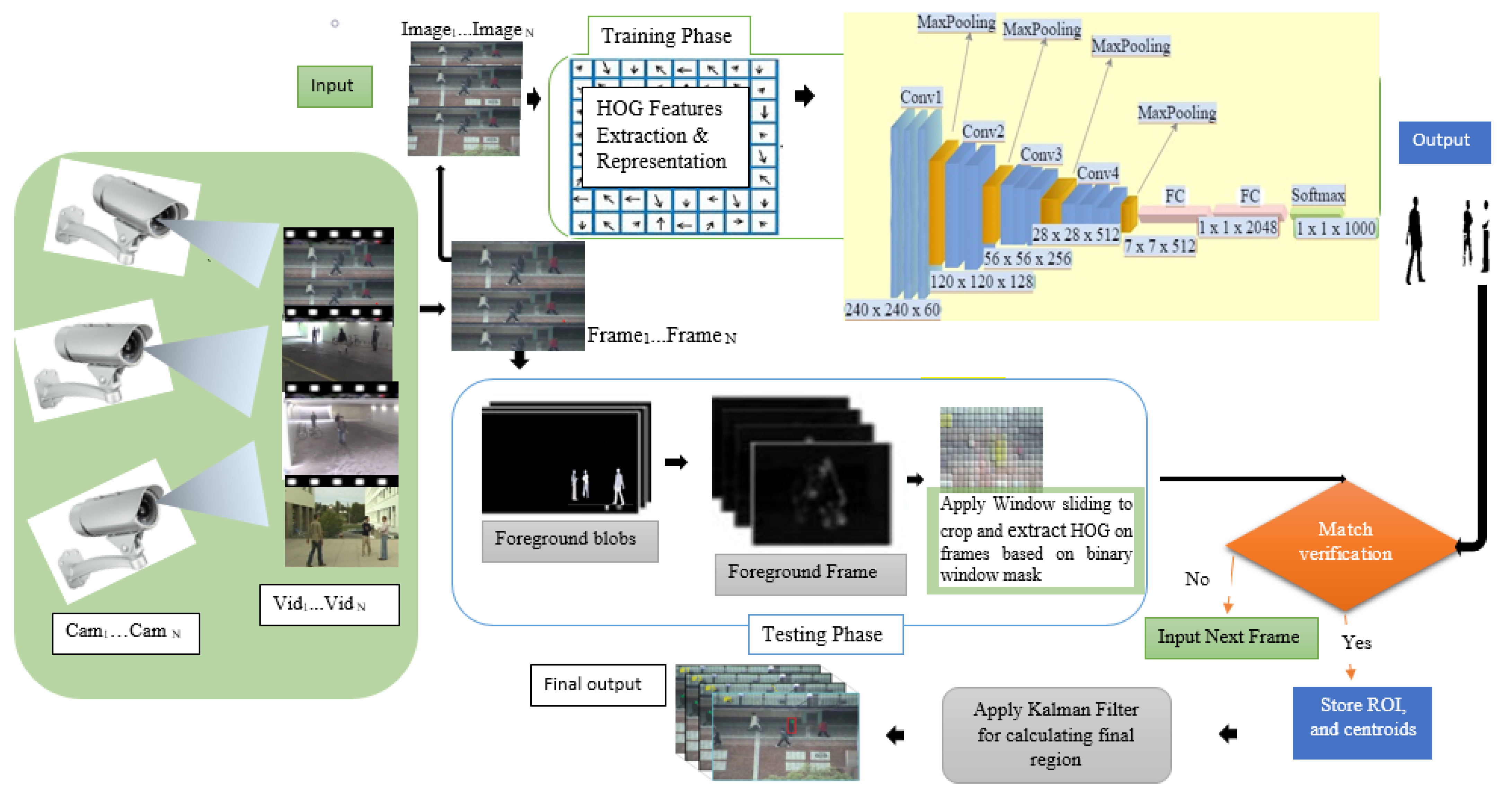
28] and gray images captured from multiple surveillance cameras. The proposed algorithm takes an input of the 120 × 32 images, cleans and converts them into binary format, and then smoothens the pixels on binary images by applying morphological operations that are followed by the implementation of a Laplacian of Gaussian model (LOG) mixture after blobs. The images undergo further feature extraction and computation with the HOG descriptor. We stored these features into a 2-dimensional array and passed them to the fully connected multi-layer neural network for further classifications and matching computation, as shown in
Figure 1. The CNN flattens the given 2D array into a single feature vector that is used to determine the object of interest’s class. Then an output from the HOG descriptor compared them with the object of interest on the input frame based on the connected components, image region properties, and window binary mask. The sliding window tactics were applied on input frames to reduce the data size, processing time, and to improve the object locating during tracking in one step. The normalized cross-function is used to obtain the object centroids on these images. Finally, we considered the use of the Kalman filter to track the object of interest, based on the computed centroids.
3.1. Background Segmenting Modeling
Background motion has always been a throwback for many conventional methods to achieve the desired accuracy [
23,
25]. However, we applied the background subtraction model to ensure that our algorithm overcomes these challenges. In this modeling, we set the threshold pixel value to 0.5 to ensure the detection of every blob for all objects shapes. We further applied the splitting of the image into foreground and background for our algorithm to efficiently classify the pixels [
29]. However, the recent history of each pixel value is observed with a mixture of Gaussian distributions, and the new pixel values are considered as the major components to update the model. These new pixel values at a given time (
) are further checked against generated Gaussian distribution until matches are obtained [
30]. The pixels with similar velocity at given x and y directions are considered as a point of interest of the same object representing its velocity. These matches are then defined with a standard deviation (
) of the distribution. This improved the foreground masks, connectivity between neighboring pixels, speed mapping of the moving object, and the capability to distinguish the non-stationary detections from the foreground blobs.
However, when there are no matches found in the
generated distribution, the probability of the distribution of the previous action is replaced with the current mean (
) value, highest variance (
) and the lowest weight (
) of the object. Thus, we observe the probability of the pixel values as follows.
where
represent recent pixels history and
;
T denotes the number of the distributions, whereas
represents an estimated weight of the
ith The Gaussian mixture at given time
,
and
respectively denotes the mean and covariance matrix. Then
denotes the Gaussian probability density function and is computed as follows.
Then the weight of the
distribution at a given time is updated as follows.
where
denote the learning rate,
T is equivalent to the available memory and computation power usage,
where one denotes model matching is true, zero represents that model as unmatched. The advantage of this background technique we applied is that our background model is updated without destroying the existing model. This is achieved by ensuring that after the weights normalizations, the mean and the variance corresponds with the conditions of the distribution and are updated only when conditions change by using the following equations, respectively.
and
We further ensured that the learning factor
p adapts to the current distributions by computing it as:
3.3. HOG Descriptor’s Features Extraction
Hog is a feature extraction technique that extracts features from every position of the image by constructing logic histograms of the object from the images [
7]. In this paper, the images are first passed through the HOG descriptor for data size reduction and searching for an object to detect. Thereafter, the histograms are created and computed over the whole images that are retrieved from several video frames. These histograms are then appended into a single feature vector using the exponential equation
, representing the grid level (
for all cells along the dimensions. However, the correspondence on the whole input images between the vectors and histograms bins is ensured by limiting the level (
) to ≤3 and computed using the following equation.
where
, denotes vector dimensions,
denotes bins,
defines grid level. This equation ensures that all images that are extremely large and rich in texture are weighted the same as low texture images within the set parameters. It is also used to guard and control our algorithm against overfitting.
In our detection module, a two-dimensional (2D) array of the detected object is constructed. It is passed to the CNN, wherein the process of targeted object recognition is flattened into a single vector using two fully connected layers. The CNN is also used to classify that the person detected by the HOG descriptor is either associated with the assigned ID (e.g., ID1 or other IDs) [
31].
3.5. Designing Kalman Filter for Our HCNN Algorithm
In most cases, computer vision algorithms’ frequent task is based on object detection and localization [
26,
32]. Therefore, in this paper, we considered the design and the incorporation of a simple and robust procedure to engage complex scenes with minimum resources [
27]. We integrated the computed object centroids into the Kalman filter’s object motion and measurement noise [
29]. This strengthened the processing of noises and the estimation of the object’s next position in the next frame at a given speed and time [
12]. However, it also made our algorithm entitled to efficiently re-detect the moving object during occlusions, scaling, illuminations, appearance changes, and rapid motion on both training and validation phases [
33]. Therefore, to solve these challenges, we enabled the Kalman filer to model and associate the target ID that is assigned based on the computed centroids. This improved the observations, predictions, measurements, corrections, and updating of the object’s whereabouts and directions.
Thus, observations are effectively used to locate the object and provide a direction at a given velocity and measurement using the following equation.
where
denotes measurements,
represents the location of the object being tracked, and
is distributed normally (
~
N (0,
) and denotes noisy measurements due to uncertainty of the current object location. Although this guarantees that our algorithm can handle the noises, we prognosticate that our detector might be imperfect due to the combination of
and velocity (
variations that will affect the tracker to locate and track the object of interest effectively. Thus, to handle these uncertainties, we estimated the trajectories of the moving object from the initial state to the final state of direction by incorporating the
into the converted matrix formulae of motion measurement as follows.
denoting location
X, and speed
V of an object at a particular time
denoting the distance measurement of an object at a particular time
Thus, the Equations (10) and (11) are combined and expanded to express the location of an object being tracked as follows:
which is further converted into a matrix equation and used to handle both noisy measurements and speed variation.
denote
H state control matrix at time
t + 1.
In short, Equation (13) is expressed as
However, the Equation (13) estimations do not adapt to the speed changes. Therefore, to incorporate speed variations and locate the position of the object correctly in the next frame, we calculated the algorithm evaluation through time (
at acceleration (
and changes in time (
using the equation below.
where
denotes our prediction corrections,
denotes the location of the object at a given time
,
denote the speed of the object at a given time
, and
represent speed integration at a given time
. However, the speed is not constant for the object in motion. Hence, we accommodated its changes through different frames scenes by adapting velocity variations using the equation below.
We further expanded Equation (14) for time evolution handling and to ensure that the motion and object feature representation on both foreground frames and binary images are correctly captured and predicted. Hence, the newly desired formulae are expressed as follows:
where
denotes state transition matrix function (
F),
denote object’s acceleration and is distributed normally with mean 0 and variance of the noise measurements,
. Therefore, Equation (16) is further expressed in short, as
where
G represents a vector
, which is the object’s uncertainty in time changes. Finally, we used these equations into the Kalman filter to predict and correct the object velocity based on the pixels found in the
x and
y directions. We predicted the steps and propagated the state as follows:
where
is a random variable of a normal distribution with a mean
and covariance
.
where
represents the previous state with a certain speed at a particular time. Therefore, we expanded the covariance equation to estimate and update time as follows.
where
defines the estimated error covariance matrix in the next frame. Thus, knowledge of the measurement (
steps are now incorporated into the moving object’s estimate state vector (
) and the (a) Measuring residual error, (b) Residual covariance, and (c) Kalman gain are computed as respectively as follows.
Therefore, after this measurement steps incorporation, we can finally update the variable position estimates in the next frame by updating the mean and covariance based on the Kalman gain using the equations below.
and
I is a 4 × 4 identity matrix:
.


