
State-of-the-Art Capability of Convolutional Neural Networks to Distinguish the Signal in the Ionosphere

 , , , ,
  and
and
Abstract
:1. Introduction
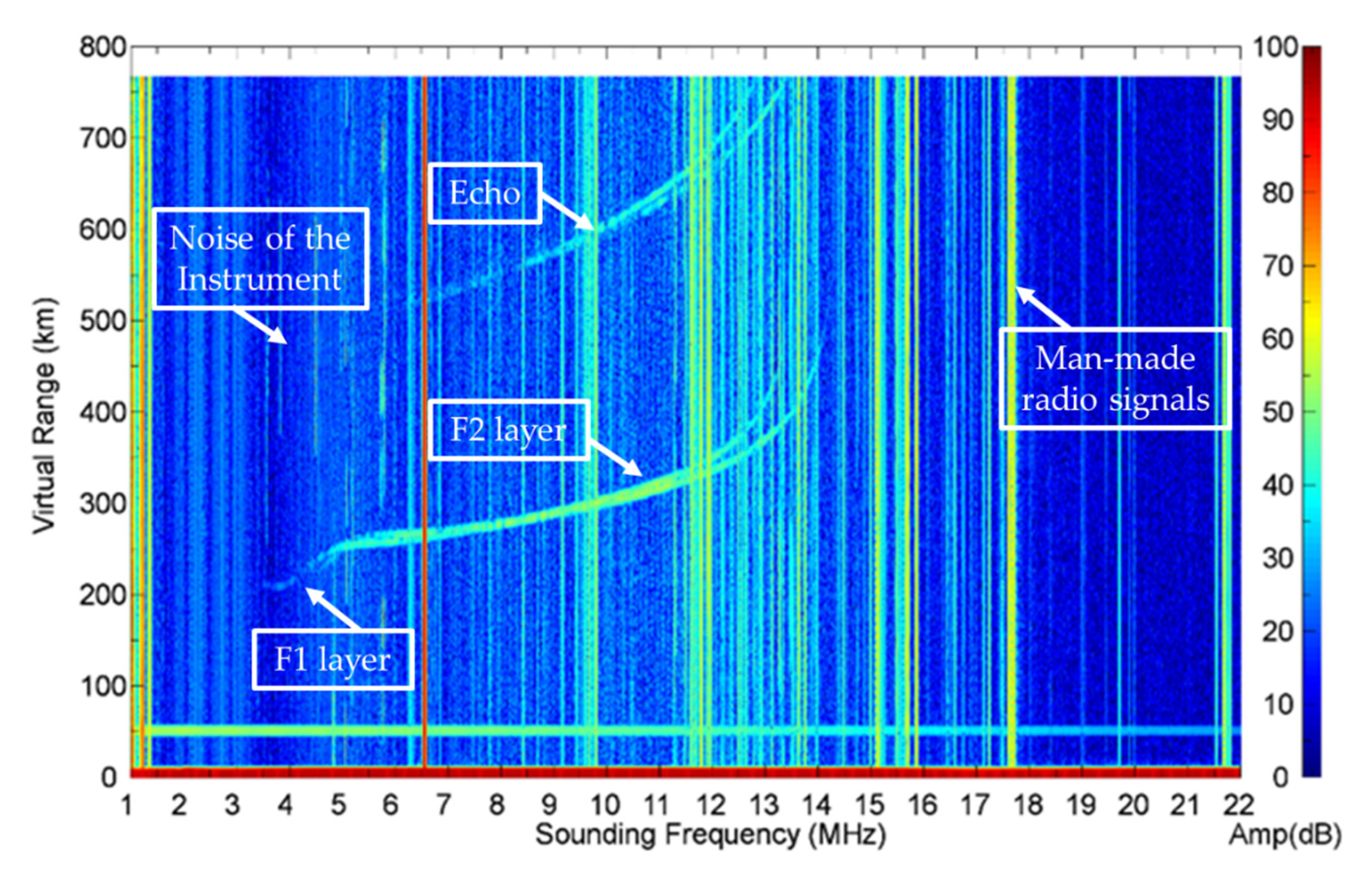
2. Data
3. Method
3.1. Preparation of Ground Truth
3.2. Models
3.2.1. DeepLab
3.2.2. FC-DenseNet
3.2.3. DWT
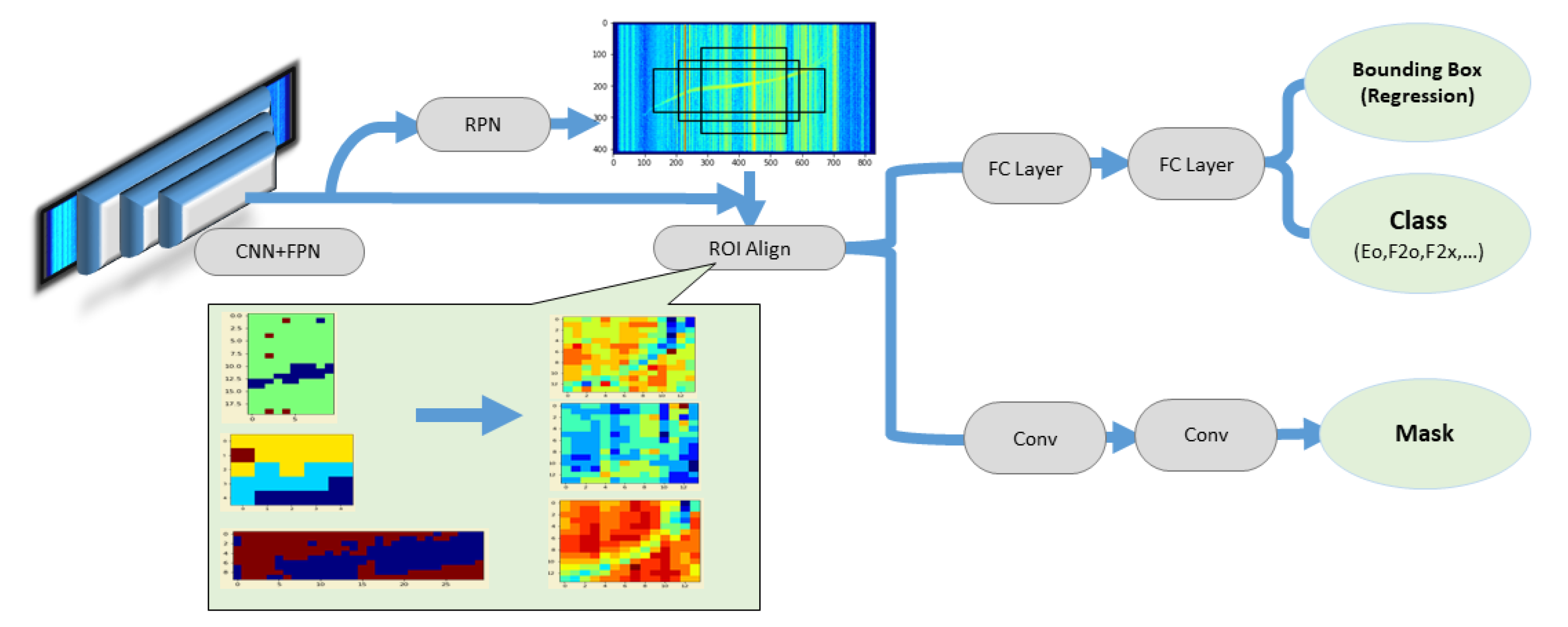
3.2.4. Mask R-CNN
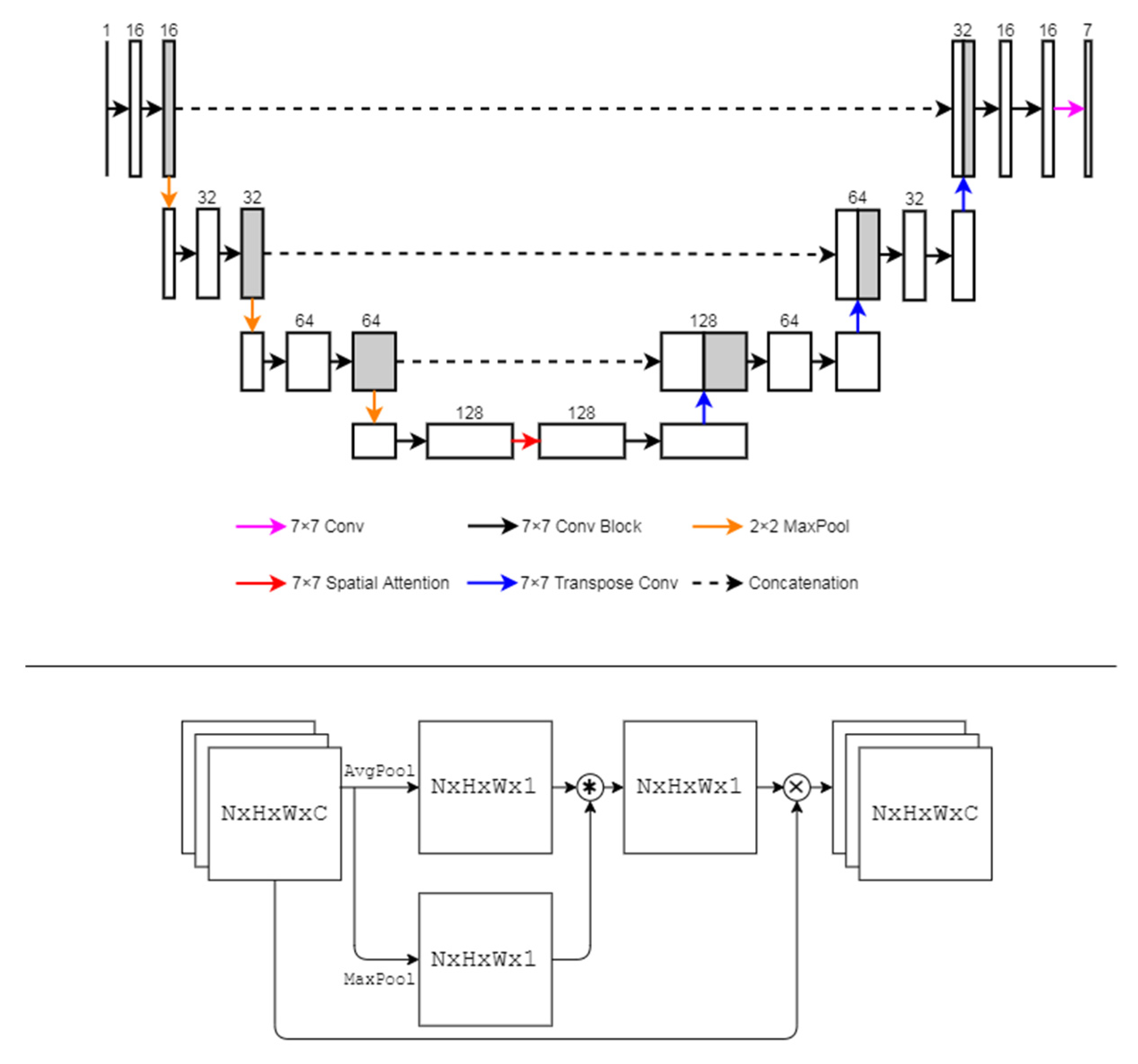
3.2.5. SA-UNet
3.3. Evaluation of Performance
3.3.1. Signal-to-Noise Ratio (SNR)
3.3.2. Circumference-over-Area Ratio (C/A)
3.3.3. Overlapping Ratio (OR)
4. Results and Discussion
4.1. Comparison of Model Performance
4.2. The Effect of Signal-to-Noise Ratio
4.3. The Effect of Circumference-over-Area Ratio (C/A)
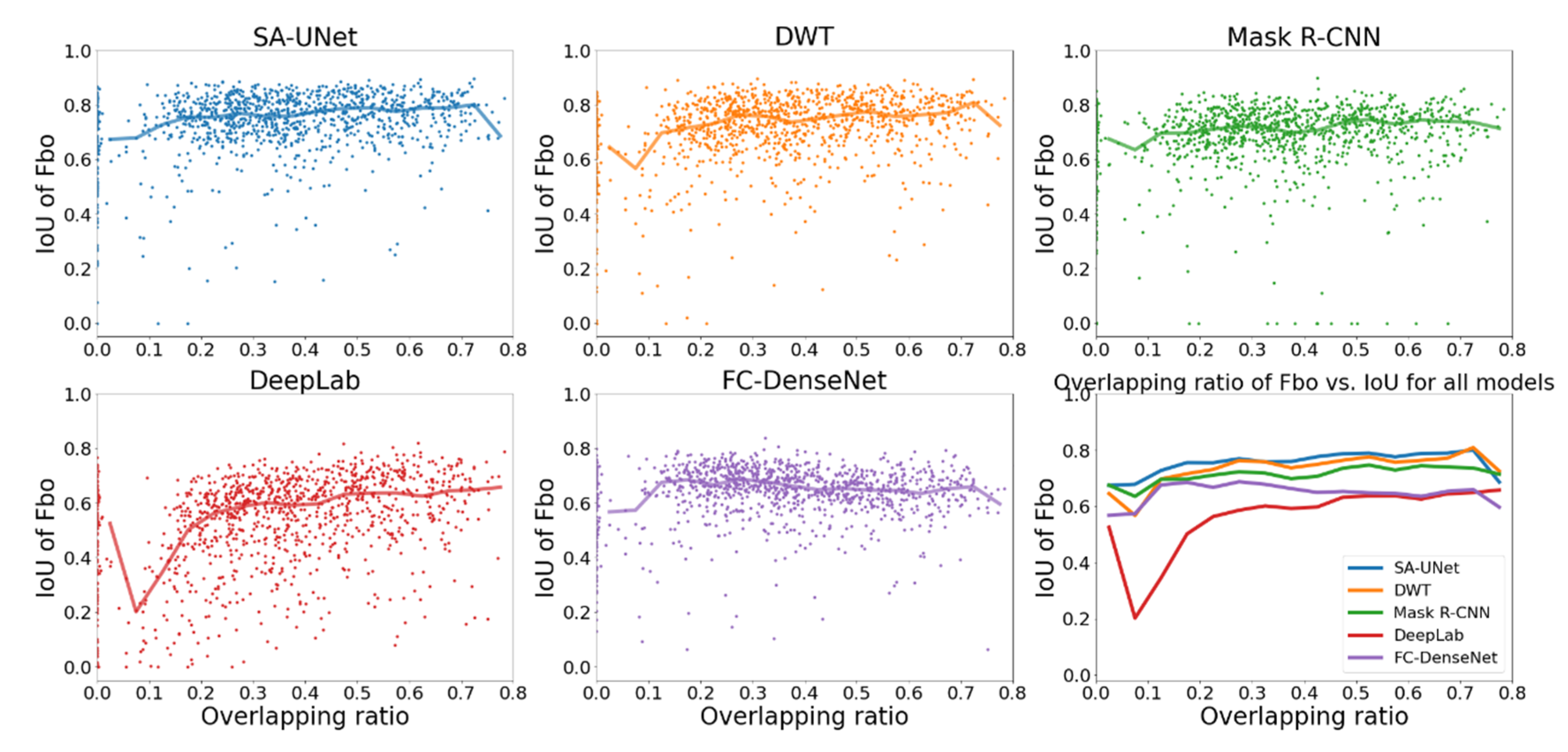
4.4. The Effect of Overlapping Ratio (OR)
5. Conclusions
Author Contributions
Funding
Institutional Review Board Statement
Informed Consent Statement
Data Availability Statement
Conflicts of Interest
References
- Mendoza, M.M.; Chang, Y.C.; Dmitriev, A.V.; Lin, C.H.; Tsai, L.C.; Li, Y.H.; Tsogtbaatar, E. Recovery of Ionospheric Signals Using Fully Convolutional DenseNet and Its Challenges. Sensors 2021, 21, 6482. [Google Scholar] [CrossRef] [PubMed]
- Whitehead, J.D. Production and prediction of sporadic E. Rev. Geophys. 1970, 8, 65–144. [Google Scholar] [CrossRef]
- Weber, E.J.; Buchau, J.; Moore, J.G. Airborne studies of equatorial F layer ionospheric irregularities. J. Geophys. Res. Space Phys. 1980, 85, 4631–4641. [Google Scholar] [CrossRef]
- Tsai, L.C.; Tien, M.H.; Chen, G.H.; Zhang, Y. HF radio angle-of-arrival measurements and ionosonde positioning. Terr. Atmos. Ocean. Sci. 2014, 25, 401–413. [Google Scholar] [CrossRef] [Green Version]
- Tsai, L.C.; Berkey, F.T. Ionogram analysis using fuzzy segmentation and connectedness techniques. Radio Sci. 2020, 35, 1173–1186. [Google Scholar] [CrossRef] [Green Version]
- De la Jara, C.; Olivares, C. Ionospheric Echoes Detection in Digital Ionograms Using Convolutional Neural Networks. Radio Sci. 2021, 56, 1–15. [Google Scholar] [CrossRef]
- Mochalov, V.; Anastasia, M. Application of deep learning to recognize ionograms. In Proceedings of the 2019 Russian Open Conference on Radio Wave Propagation (RWP), Tatarstan, Russia, 1–6 July 2019. [Google Scholar] [CrossRef]
- Xiao, Z.; Wang, J.; Li, J.; Zhao, B.; Hu, L.; Liu, L. Deep-learning for ionogram automatic scaling. Adv. Space Res. 2020, 66, 942–950. [Google Scholar] [CrossRef]
- Chen, L.C.; Zhu, Y.; Papandreou, G.; Schroff, F.; Adam, H. Encoder-decoder with atrous separable convolution for semantic image segmentation. In Proceedings of the European Conference on Computer Vision (ECCV), Munich, Germany, 8–14 September 2018. [Google Scholar] [CrossRef] [Green Version]
- Jégou, S.; Drozdzal, M.; Vazquez, D.; Romero, A.; Bengio, Y. The one hundred layers tiramisu: Fully convolutional densenets for semantic segmentation. In Proceedings of the IEEE conference on computer vision and pattern recognition workshops (CVPRW), Honolulu, HI, USA, 21–26 July 2017. [Google Scholar] [CrossRef] [Green Version]
- Roerdink, J.B.; Meijster, A. The watershed transform: Definitions, algorithms and parallelization strategies. Fundam. Inform. 2000, 41, 187–228. [Google Scholar] [CrossRef] [Green Version]
- Beucher, S. The watershed transformation applied to image segmentation. Scanning Microsc. 1992, 1992, 28. [Google Scholar]
- Smith, S.L.; Kindermans, P.J.; Ying, C.; Le, Q.V. Don’t Decay the Learning Rate, Increase the Batch Size. arXiv 2017, arXiv:1711.00489. [Google Scholar]
- He, K.; Gkioxari, G.; Dollár, P.; Girshick, R. Mask r-cnn. In Proceedings of the IEEE International Conference on Computer Vision (ICCV), Venice, Italy, 22–29 October 2017. [Google Scholar] [CrossRef]
- Guo, C.; Szemenyei, M.; Pei, Y.; Yi, Y.; Zhou, W. SD-UNet: A structured dropout U-Net for retinal vessel segmentation. In Proceedings of the 2019 IEEE 19th International Conference on Bioinformatics and Bioengineering (BIBE), Athens, Greece, 28–30 October 2019. [Google Scholar] [CrossRef]
- Guo, C.; Szemenyei, M.; Yi, Y.; Wang, W.; Chen, B.; Fan, C.R. Spatial attention u-net for retinal vessel segmentation. In Proceedings of the 2020 25th International Conference on Pattern Recognition (ICPR), Milan, Italy, 10–15 January 2021. [Google Scholar] [CrossRef]
- Furukawa, R.; Kazuhiro, H.R. Localized Feature Aggregation Module for Semantic Segmentation. In Proceedings of the 2021 IEEE International Conference on Systems, Man, and Cybernetics (SMC), Melbourne, Australia, 17–21 October 2021. [Google Scholar] [CrossRef]
- Quan, B.; Liu, B.; Fu, D.; Chen, H.; Liu, X. Improved Deeplabv3 For Better Road Segmentation In Remote Sensing Images. In Proceedings of the 2021 International Conference on Computer Engineering and Artificial Intelligence (ICCEAI), Shanghai, China, 22–24 July 2022. [Google Scholar] [CrossRef]
- Niu, Z.; Liu, W.; Zhao, J.; Jiang, G. DeepLab-based spatial feature extraction for hyperspectral image classification. IEEE Geosci. Remote Sens. Lett. 2018, 16, 251–255. [Google Scholar] [CrossRef]
- Hai, J.; Qiao, K.; Chen, J.; Tan, H.; Xu, J.; Zeng, L.; Yan, B. Fully convolutional densenet with multiscale context for automated breast tumor segmentation. J. Healthc. Eng. 2019, 1–12. [Google Scholar] [CrossRef] [PubMed] [Green Version]
- Guo, X.; Chen, Z.; Wang, C. Fully convolutional DenseNet with adversarial training for semantic segmentation of high-resolution remote sensing images. J. Appl. Remote Sens. 2021, 15, 016520. [Google Scholar] [CrossRef]
- Li, Y.H.; Putri, W.R.; Aslam, M.S.; Chang, C.C. Robust Iris Segmentation Algorithm in Non-Cooperative Environments Using Interleaved Residual U-Net. Sensors 2021, 21, 1434. [Google Scholar] [CrossRef] [PubMed]
- Chen, Y.; Wang, W.; Zeng, Z.; Wang, Y. An adaptive CNNs technology for robust iris segmentation. IEEE Access 2019, 7, 64517–64532. [Google Scholar] [CrossRef]
- Marcos, D.; Tuia, D.; Kellenberger, B.; Zhang, L.; Bai, M.; Liao, R.; Urtasun, R.R. Learning deep structured active contours end-to-end. In Proceedings of the IEEE Conference on Computer Vision and Pattern Recognition (CVPR), Salt Lake City, UT, USA, 18–23 June 2018. [Google Scholar] [CrossRef] [Green Version]
- Li, X.H.; Yin, F.; Xue, T.; Liu, L.; Ogier, J.M.; Liu, C.L. Instance aware document image segmentation using label pyramid networks and deep watershed transformation. In Proceedings of the 2019 International Conference on Document Analysis and Recognition (ICDAR), Sydney, Australia, 20–25 September 2019. [Google Scholar] [CrossRef]
- He, K.; Zhang, X.; Ren, S.; Sun, J. Deep residual learning for image recognition. In Proceedings of the IEEE conference on computer vision and pattern recognition (CVPRW), Las Vegas, NV, USA, 21 June–1 July 2016. [Google Scholar] [CrossRef] [Green Version]
- Huang, G.; Liu, Z.; Van Der Maaten, L.; Weinberger, K.Q. Densely connected convolutional networks. In Proceedings of the IEEE conference on computer vision and pattern recognition (CVPRW), Honolulu, HI, USA, 21–26 July 2017. [Google Scholar] [CrossRef] [Green Version]
- Simonyan, K.; Zisserman, A. Very deep convolutional networks for large-scale image recognition. arXiv 2014, arXiv:1409.1556. [Google Scholar]
- Ghiasi, G.; Lin, T.Y.; Le, Q.V. Dropblock: A regularization method for convolutional networks. arXiv 2018, arXiv:1810.12890. [Google Scholar]


| Ionospheric Layer | Class Label |
|---|---|
| E layer ordinary mode | Eo |
| E layer extraordinary mode | Ex |
| Sporadic E layer ordinary mode | Eso |
| Sporadic E layer extraordinary mode | Esx |
| Sporadic E layer | Es |
| F1 layer ordinary mode | Fao |
| F1 layer extraordinary mode | Fax |
| F2 layer ordinary mode | Fbo |
| F2 layer extraordinary mode | Fbx |
| F3 layer ordinary mode | Fco |
| F3 layer extraordinary mode | Fcx |
| Eo | Ex | Es | Eso | Esx | Fao | Fax | Fbo | Fbx | Fco | Fcx | |
|---|---|---|---|---|---|---|---|---|---|---|---|
| Training | 7.6 | 1.1 | 39.9 | 12.6 | 10.0 | 39.3 | 26.4 | 94.6 | 87.8 | 0.15 | 0.13 |
| Test | 9.2 | 1.1 | 40.8 | 14.8 | 11.2 | 38.7 | 25.5 | 94.2 | 87.7 | 0.08 | 0.08 |
| Validation | 7.5 | 0.5 | 38.0 | 14.5 | 12.2 | 39.4 | 25.3 | 95.5 | 89.8 | 0.10 | 0.40 |
| Parameters | Layers | |
|---|---|---|
| DeepLab | 1,259,393 | 126 |
| FC-DenseNet | 685,032 | 130 |
| DWT | 38,147,984 | 46 |
| Mask R-CNN | 44,972,890 | 242 |
| SA-UNet | 2,914,910 | 26 |
| Training Time (Hours) | Inference Time (s) | |
|---|---|---|
| DeepLab | 3.8 | 0.06 |
| FC-DenseNet | 6.4 | 0.08 |
| DWT | 13 | 0.21 |
| Mask R-CNN | 8 | 0.23 |
| SA-UNet | 23 | 0.08 |
| Eo | Ex | Es | Eso | Esx | Fao | Fax | Fbo | Fbx | Fco | Fcx | |
|---|---|---|---|---|---|---|---|---|---|---|---|
| DeepLab | 0 | 0 | 0.643 | 0 | 0 | 0.139 | 0 | 0.568 | 0.544 | 0 | 0 |
| FC-DenseNet | 0 | 0 | 0.701 | 0.340 | 0 | 0.519 | 0.332 | 0.630 | 0.534 | 0 | 0 |
| DWT | 0.157 | 0 | 0.670 | 0.278 | 0.289 | 0.481 | 0.323 | 0.725 | 0.693 | 0 | 0 |
| Mask R-CNN | 0.270 | 0.246 | 0.710 | 0.340 | 0.330 | 0.510 | 0.340 | 0.680 | 0.680 | 0 | 0 |
| SA-UNet | 0 | 0 | 0.722 | 0 | 0 | 0.489 | 0.080 | 0.745 | 0.710 | 0 | 0 |
Publisher’s Note: MDPI stays neutral with regard to jurisdictional claims in published maps and institutional affiliations. |
© 2022 by the authors. Licensee MDPI, Basel, Switzerland. This article is an open access article distributed under the terms and conditions of the Creative Commons Attribution (CC BY) license (https://creativecommons.org/licenses/by/4.0/).
Share and Cite
Chang, Y.-C.; Lin, C.-H.; Dmitriev, A.V.; Hsieh, M.-C.; Hsu, H.-W.; Lin, Y.-C.; Mendoza, M.M.; Huang, G.-H.; Tsai, L.-C.; Li, Y.-H.; et al. State-of-the-Art Capability of Convolutional Neural Networks to Distinguish the Signal in the Ionosphere. Sensors 2022, 22, 2758. https://0-doi-org.brum.beds.ac.uk/10.3390/s22072758
Chang Y-C, Lin C-H, Dmitriev AV, Hsieh M-C, Hsu H-W, Lin Y-C, Mendoza MM, Huang G-H, Tsai L-C, Li Y-H, et al. State-of-the-Art Capability of Convolutional Neural Networks to Distinguish the Signal in the Ionosphere. Sensors. 2022; 22(7):2758. https://0-doi-org.brum.beds.ac.uk/10.3390/s22072758
Chicago/Turabian StyleChang, Yu-Chi, Chia-Hsien Lin, Alexei V. Dmitriev, Mon-Chai Hsieh, Hao-Wei Hsu, Yu-Ciang Lin, Merlin M. Mendoza, Guan-Han Huang, Lung-Chih Tsai, Yung-Hui Li, and et al. 2022. "State-of-the-Art Capability of Convolutional Neural Networks to Distinguish the Signal in the Ionosphere" Sensors 22, no. 7: 2758. https://0-doi-org.brum.beds.ac.uk/10.3390/s22072758