
Development and Calibration of Pressure-Temperature-Humidity (PTH) Probes for Distributed Atmospheric Monitoring Using Unmanned Aircraft Systems


Abstract
:1. Introduction
2. Materials and Methods
2.1. Sensor Selection
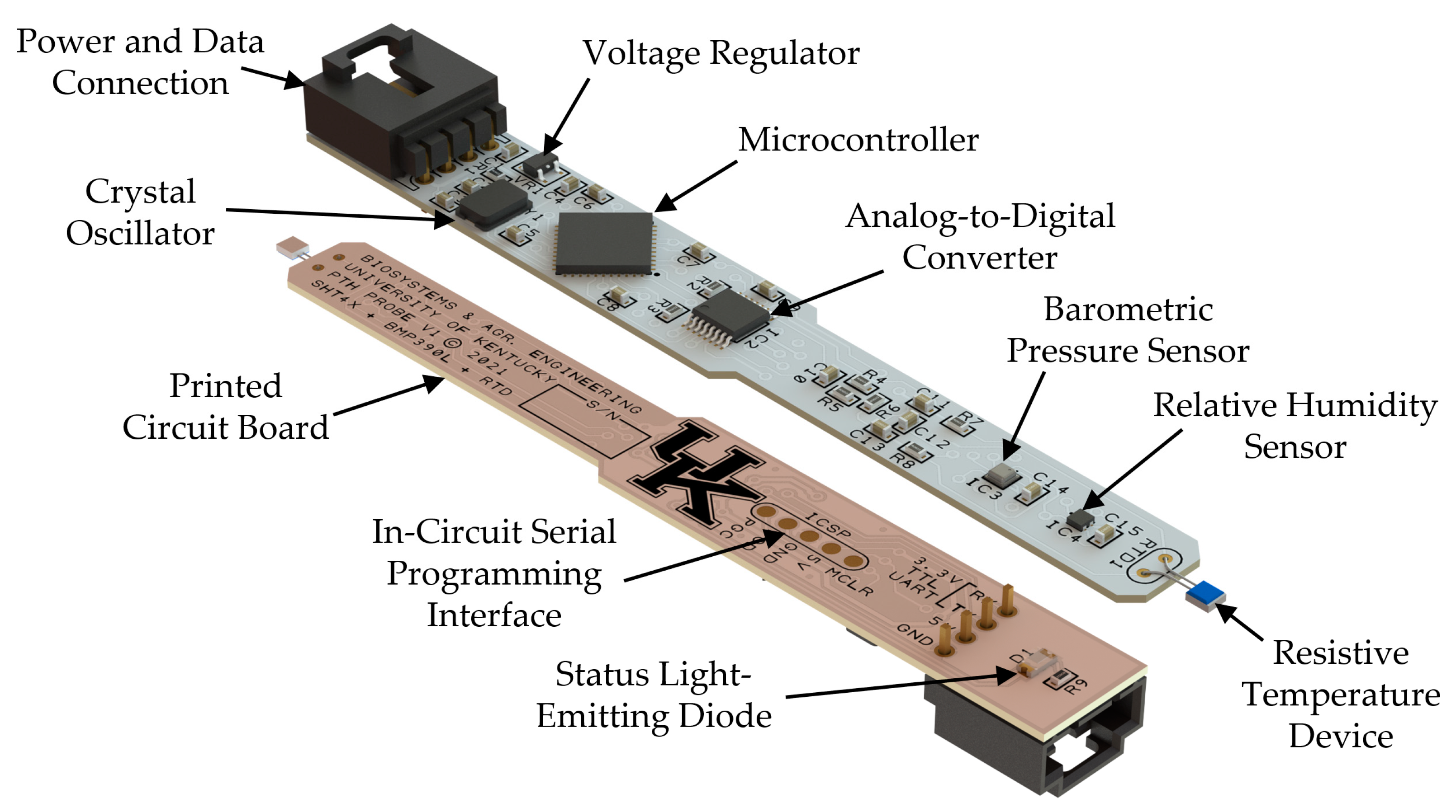
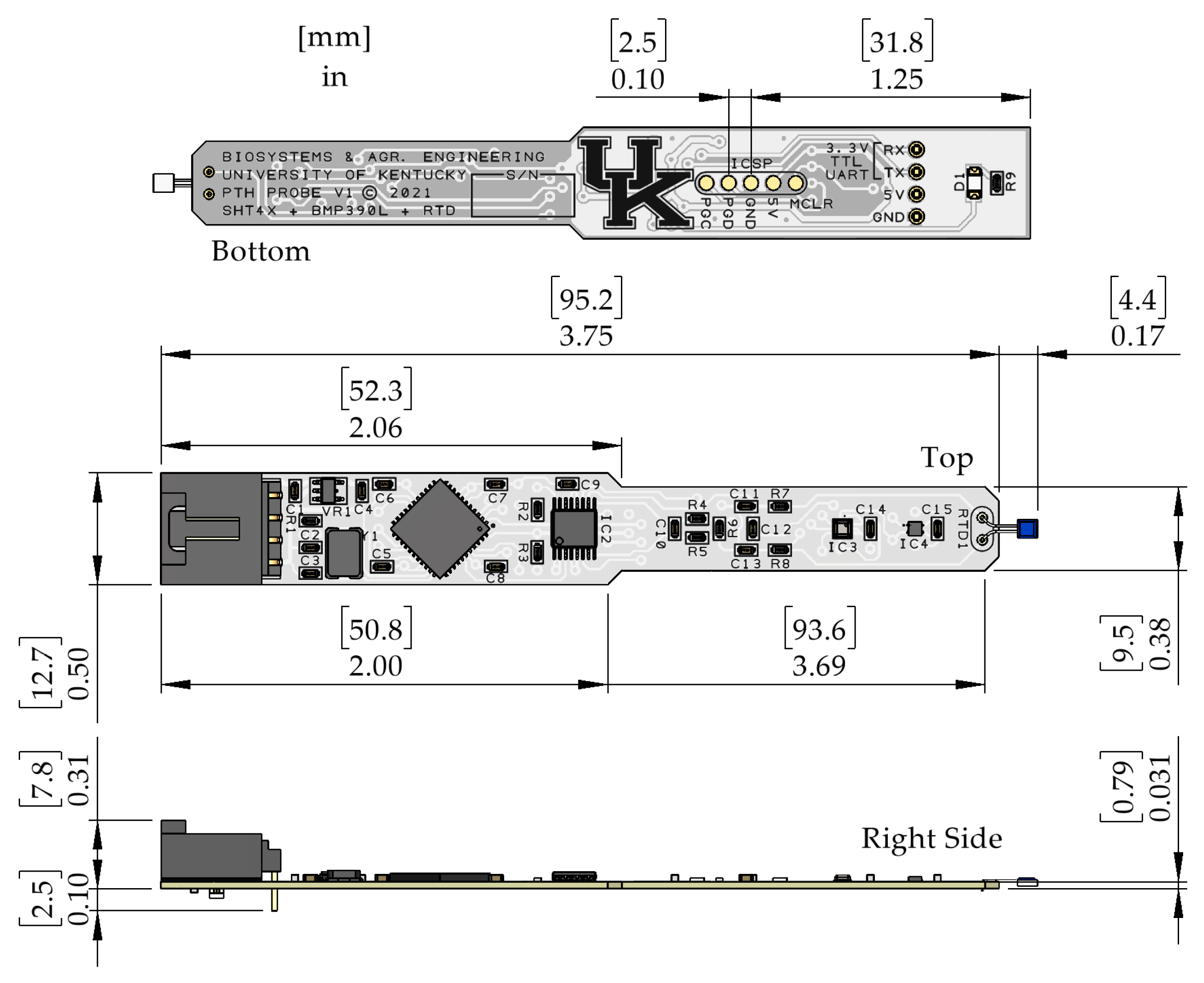
2.2. PTH Probe Design
2.3. PTH Probe Assembly
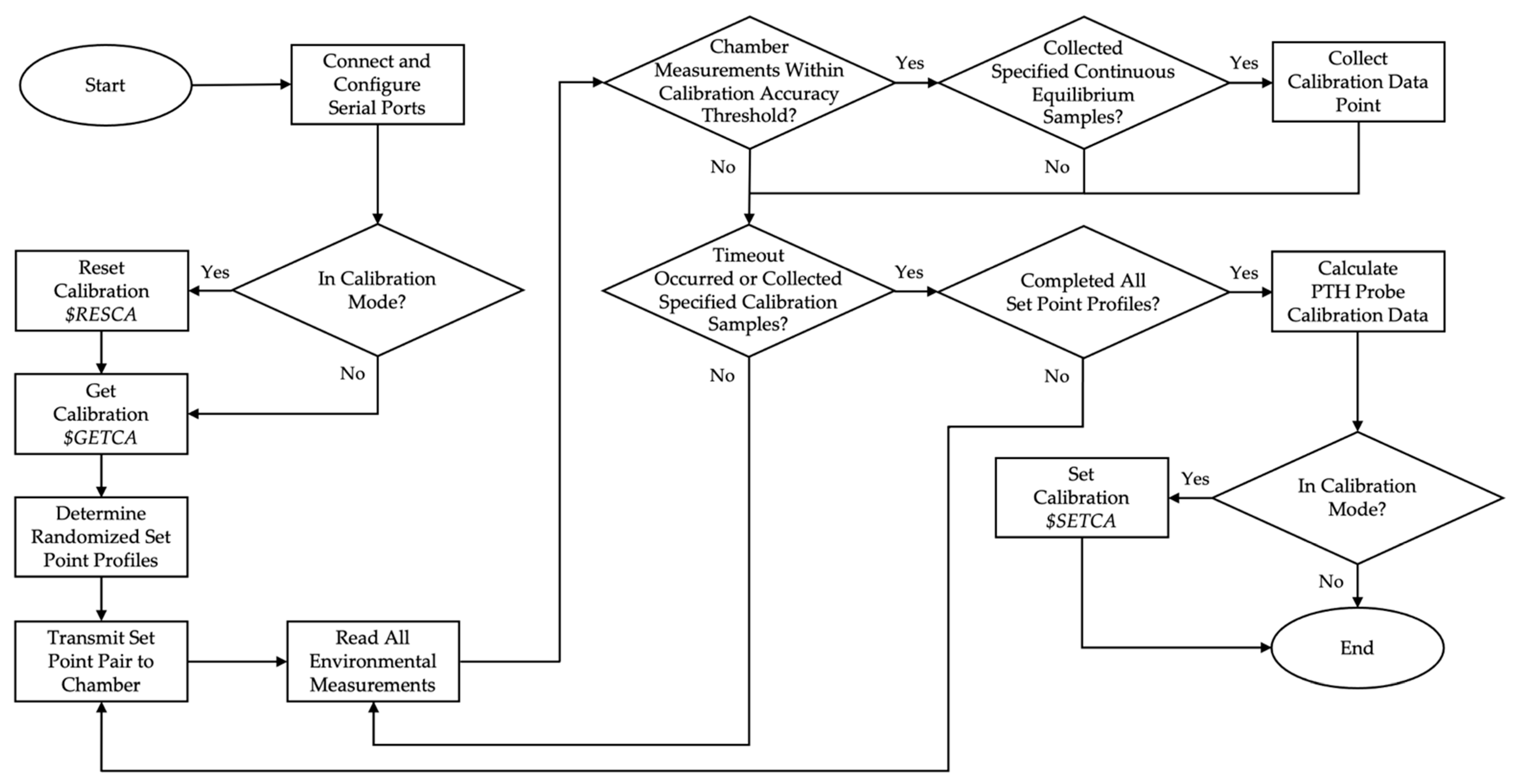
2.4. PTH Probe Firmware Development
2.5. Calibration System Development
2.6. Calibration
2.7. Validation
2.8. Statistical Analysis
3. Results
3.1. PTH Probe Specifications
3.2. Calibration/Validation System
3.3. Calibration
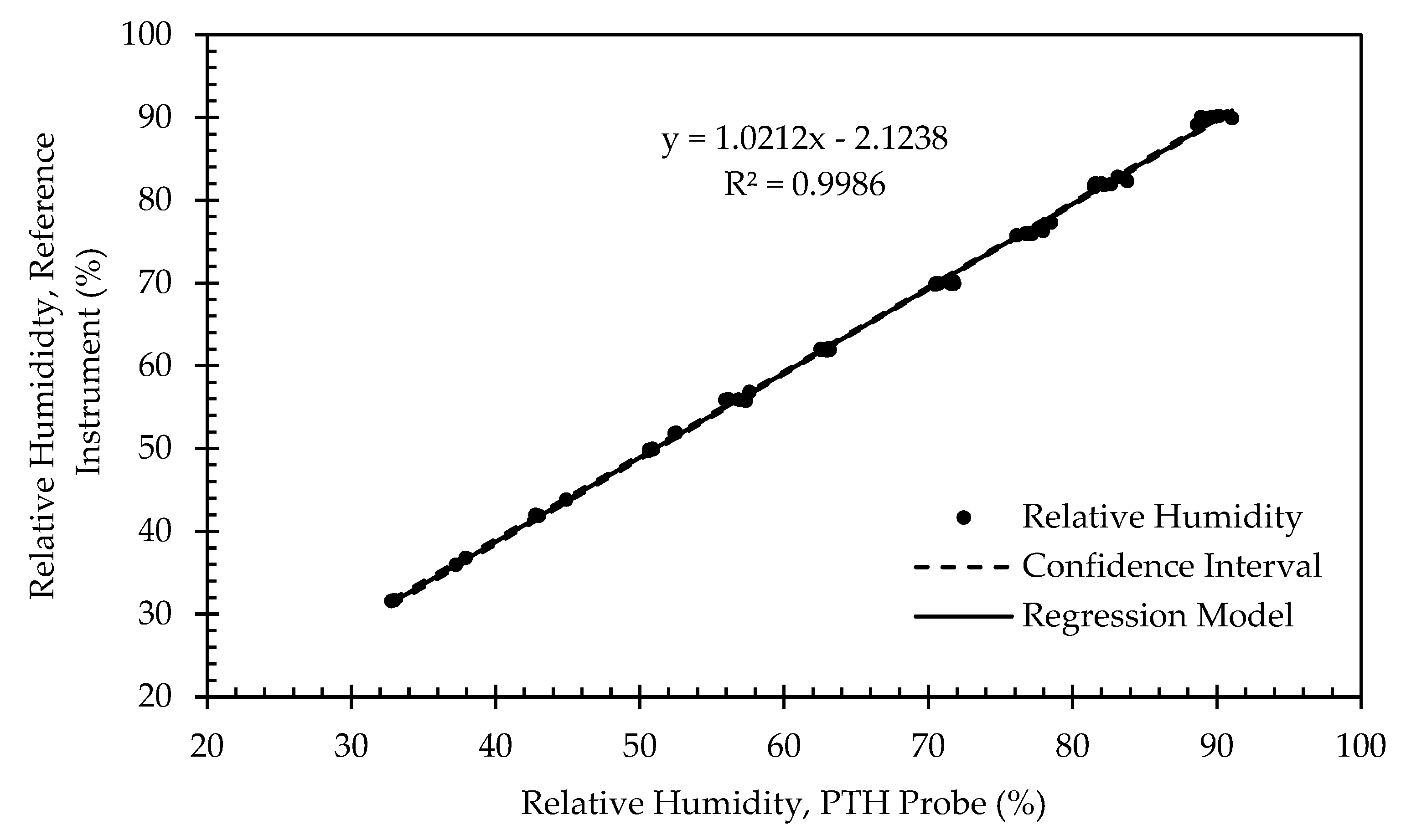
3.4. Validation
4. Discussion
5. Conclusions
6. Patents
Author Contributions
Funding
Institutional Review Board Statement
Informed Consent Statement
Data Availability Statement
Conflicts of Interest
References
- Brewer, M.J.; Clements, C.B. Meteorological Profiling in the Fire Environment Using UAS. Fire 2020, 3, 36. [Google Scholar] [CrossRef]
- Bailey, S.C.C.; Canter, C.A.; Sama, M.P.; Houston, A.L.; Smith, S.W. Unmanned aerial vehicles reveal the impact of a total solar eclipse on the atmospheric surface layer. Proc. R. Soc. A 2019, 475, 20190212. [Google Scholar] [CrossRef]
- Hemingway, B.L.; Frazier, A.E.; Elbing, B.R.; Jacob, J.D. Vertical Sampling Scales for Atmospheric Boundary Layer Measurements from Small Unmanned Aircraft Systems (sUAS). Atmosphere 2017, 8, 176. [Google Scholar] [CrossRef] [Green Version]
- Pinto, J.O.; Jensen, A.A.; Jimenez, P.A.; Hertneky, T.; Munoz-Esparza, D.; Dumont, A.; Steiner, M. Real-time WRF large-eddy simulations to support uncrewed aircraft system (UAS) flight planning and operations during 2018 LAPSE-RATE. Earth Syst. Sci. Data 2021, 13, 697–711. [Google Scholar] [CrossRef]
- Nolan, P.J.; Pinto, J.; Gonzalez-Rocha, J.; Jensen, A.; Vezzi, C.N.; Bailey, S.C.C.; de Boer, G.; Diehl, C.; Laurence, R.; Powers, C.W.; et al. Coordinated Unmanned Aircraft System (UAS) and Ground-Based Weather Measurements to Predict Lagrangian Coherent Structures (LCSs). Sensors 2018, 18, 4448. [Google Scholar] [CrossRef] [Green Version]
- Aurell, J.; Gullett, B.; Holder, A.; Kiros, F.; Mitchell, W.; Watts, A.; Ottmar, R. Wildland fire emission sampling at Fishlake National Forest, Utah using an unmanned aircraft system. Atmos. Environ. 2021, 247, 118193. [Google Scholar] [CrossRef]
- Nelson, K.N.; Boehmler, J.M.; Khlystov, A.Y.; Moosmüller, H.; Samburova, V.; Bhattarai, C.; Wilcox, E.M.; Watts, A.C. A multipollutant smoke emissions sensing and sampling instrument package for unmanned aircraft systems: Development and testing. Fire 2019, 2, 32. [Google Scholar] [CrossRef] [Green Version]
- Jacob, J.D.; Chilson, P.B.; Houston, A.L.; Smith, S.W. Considerations for Atmospheric Measurements with Small Unmanned Aircraft Systems. Atmosphere 2018, 9, 252. [Google Scholar] [CrossRef] [Green Version]
- Smith, S.W.; Chilson, P.B.; Houston, A.L.; Jacob, J.D. Catalyzing Collaboration for Multi-Disciplinary UAS Development with a Flight Campaign Focussed on Meteorology and Atmospheric Physics. In Proceedings of the AIAA Information Systems-AIAA Infotech@ Aerospace, Grapevine, TX, USA, 9–13 January 2017; p. 1156. [Google Scholar]
- Chilson, P.B.; Bell, T.M.; Brewster, K.A.; de Azevedo, G.B.H.; Carr, F.H.; Carson, K.; Doyle, W.; Fiebrich, C.A.; Greene, B.R.; Grimsley, J.L.; et al. Moving towards a Network of Autonomous UAS Atmospheric Profiling Stations for Observations in the Earth’s Lower Atmosphere: The 3D Mesonet Concept. Sensors 2019, 19, 2720. [Google Scholar] [CrossRef] [Green Version]
- de Boer, G.; Diehl, C.; Jacob, J.; Houston, A.; Smith, S.W.; Chilson, P.; Schmale, D.G.; Intrieri, J.; Pinto, J.; Elston, J.; et al. Development of Community, Capabilities, and Understanding through Unmanned Aircraft-Based Atmospheric Research: The LAPSE-RATE Campaign. Bull. Am. Meteorol. Soc. 2020, 101, E684–E699. [Google Scholar] [CrossRef] [Green Version]
- de Boer, G.; Houston, A.; Jacob, J.; Chilson, P.B.; Smith, S.W.; Argrow, B.; Lawrence, D.; Elston, J.; Brus, D.; Kemppinen, O.; et al. Data generated during the 2018 LAPSE-RATE campaign: An introduction and overview. Earth Syst. Sci. Data 2020, 12, 3357–3366. [Google Scholar] [CrossRef]
- Bailey, S.C.C.; Sama, M.P.; Canter, C.A.; Pampolini, L.F.; Lippay, Z.S.; Schuyler, T.J.; Hamilton, J.D.; MacPhee, S.B.; Rowe, I.S.; Sanders, C.D.; et al. University of Kentucky measurements of wind, temperature, pressure and humidity in support of LAPSE-RATE using multisite fixed-wing and rotorcraft unmanned aerial systems. Earth Syst. Sci. Data 2020, 12, 1759–1773. [Google Scholar] [CrossRef]
- Bell, T.M.; Klein, P.M.; Lundquist, J.K.; Waugh, S. Remote-sensing and radiosonde datasets collected in the San Luis Valley during the LAPSE-RATE campaign. Earth Syst. Sci. Data 2021, 13, 1041–1051. [Google Scholar] [CrossRef]
- Brus, D.; Gustafsson, J.; Kemppinen, O.; de Boer, G.; Hirsikko, A. Atmospheric aerosol, gases, and meteorological parameters measured during the LAPSE-RATE campaign by the Finnish Meteorological Institute and Kansas State University. Earth Syst. Sci. Data 2021, 13, 2909–2922. [Google Scholar] [CrossRef]
- de Boer, G.; Dixon, C.; Borenstein, S.; Lawrence, D.A.; Elston, J.; Hesselius, D.; Stachura, M.; Laurence Iii, R.; Swenson, S.; Choate, C.M.; et al. University of Colorado and Black Swift Technologies RPAS-based measurements of the lower atmosphere during LAPSE-RATE. Earth Syst. Sci. Data 2021, 13, 2515–2528. [Google Scholar] [CrossRef]
- de Boer, G.; Waugh, S.; Erwin, A.; Borenstein, S.; Dixon, C.; Shanti, W.; Houston, A.; Argrow, B. Measurements from mobile surface vehicles during the Lower Atmospheric Profiling Studies at Elevation—A Remotely-piloted Aircraft Team Experiment (LAPSE-RATE). Earth Syst. Sci. Data 2021, 13, 155–169. [Google Scholar] [CrossRef]
- Islam, A.; Shankar, A.; Houston, A.; Detweiler, C. University of Nebraska unmanned aerial system (UAS) profiling during the LAPSE-RATE field campaign. Earth Syst. Sci. Data 2021, 13, 2457–2470. [Google Scholar] [CrossRef]
- Pillar-Little, E.A.; Greene, B.R.; Lappin, F.M.; Bell, T.M.; Segales, A.R.; de Azevedo, G.B.H.; Doyle, W.; Kanneganti, S.T.; Tripp, D.D.; Chilson, P.B. Observations of the thermodynamic and kinematic state of the atmospheric boundary layer over the San Luis Valley, CO, using the CopterSonde 2 remotely piloted aircraft system in support of the LAPSE-RATE field campaign. Earth Syst. Sci. Data 2021, 13, 269–280. [Google Scholar] [CrossRef]
- Sanchez Gomez, M.; Lundquist, J.K.; Klein, P.M.; Bell, T.M. Turbulence dissipation rate estimated from lidar observations during the LAPSE-RATE field campaign. Earth Syst. Sci. Data 2021, 13, 3539–3549. [Google Scholar] [CrossRef]
- Barbieri, L.; Kral, S.T.; Bailey, S.C.C.; Frazier, A.E.; Jacob, J.D.; Reuder, J.; Brus, D.; Chilson, P.B.; Crick, C.; Detweiler, C.; et al. Intercomparison of Small Unmanned Aircraft System (sUAS) Measurements for Atmospheric Science during the LAPSE-RATE Campaign. Sensors 2019, 19, 2179. [Google Scholar] [CrossRef] [Green Version]
- Foster, N. Meteorological Data Collection for Three-Dimensional Forecasting Advancements Stillwater, Oklahoma: Oklahoma State University. In Proceedings of the 8th AIAA Atmospheric and Space Environments Conference, Washington, DC, USA, 13–17 June 2016. [Google Scholar] [CrossRef]
- Islam, A.; Houston, A.L.; Shankar, A.; Detweiler, C. Design and Evaluation of Sensor Housing for Boundary Layer Profiling Using Multirotors. Sensors 2019, 19, 2481. [Google Scholar] [CrossRef] [Green Version]


| Sensor | Parameter | Units | Operating Range | Maximum Accuracy | Typical Accuracy | Resolution | Response Time (s) |
|---|---|---|---|---|---|---|---|
| BMP390 | Barometric Pressure | Pa | 30,000 to 125,000 | ±50 | ±3 | 0.17 | 0.005 3 |
| Temperature | °C | −40 to 85 | ±1.5 | - | 0.0003 | - | |
| RTD 1 | Temperature | °C | −200 to 600 2 | - | ±0.15 | 0.001 | 1.2 4 |
| SHT40 | Relative Humidity | % | 0 to 100 | ±5.0 | ±1.8 | 1 | 6 4 |
| Temperature | °C | −40 to 125 | ±1.0 | ±0.2 | 0.01 | 2 4 |
| Temperature (°C) | Relative Humidity (%) |
|---|---|
| 10 | 30 |
| 13 | 36 |
| 16 | 42 |
| 20 | 50 |
| 23 | 56 |
| 26 | 62 |
| 30 | 70 |
| 33 | 76 |
| 36 | 82 |
| 40 | 90 |
| Setpoint Threshold | Sample Size | ||
|---|---|---|---|
| Temperature (°C) | Relative Humidity (%) | Equilibrium | Calibration |
| ±1 | ±2 | 300 | 150 |
| Temperature (°C) | Relative Humidity (%) |
|---|---|
| 12 | 33 |
| 14 | 39 |
| 18 | 46 |
| 22 | 53 |
| 24 | 59 |
| 28 | 66 |
| 32 | 73 |
| 34 | 79 |
| 38 | 86 |
| Parameter | Test Condition | Min | Typ | Max | Units | |
|---|---|---|---|---|---|---|
| Vs | Supply Voltage | - | 3.6 | 5.0 | 5.5 | V |
| Is | Supply Current | Vs = 5.0 V | - | - | 1 | mA |
| Vr | Regulated Voltage | 3.6 < Vs < 5.5 | 3.28 | 3.3 | 3.32 | V |
| RRTD | RTD Nominal Resistance | - | - | 100 | - | Ω |
| IRTD | RTD Drive Current | - | 0.500 | - | mA | |
| Fs | Data Output Rate | - | - | 1.000 | - | Hz |
| P | Operating Barometric Pressure | - | 30 | - | 125 | kPa |
| T | Operating Temperature | - | −40 | - | 125 | °C |
| H | Operating Relative Humidity 1 | - | 0 | - | 100 | % |
| M | PTH probe Mass | - | - | 3.41 | - | g |
| Serial Number | BMP390 | RTD | SHT40 | |||||||
|---|---|---|---|---|---|---|---|---|---|---|
| Barometric Pressure (Pa) | Temperature (°C) | Temperature (°C) | Relative Humidity (%) | Temperature (°C) | ||||||
| Slope 1 | Offset | Slope | Offset | Slope | Offset | Slope | Offset | Slope | Offset | |
| 0x0005 | 1.000 | −236.9 | 0.997 | −0.303 | 1.007 | −1.004 | 1.021 | −2.124 | 1.003 | 0.215 |
| 0x0006 | 1.000 | −303.2 | 0.991 | −0.266 | 1.005 | −0.070 | 1.021 | −1.965 | 0.998 | 0.351 |
| 0x0007 | 1.000 | −302.2 | 0.989 | −0.182 | 0.998 | −1.242 | 1.018 | −1.861 | 0.993 | 0.420 |
| 0x0008 | 1.000 | −307.6 | 0.988 | −0.192 | 0.995 | −0.774 | 1.016 | −1.691 | 0.989 | 0.505 |
| 0x0009 | 1.000 | −291.9 | 1.001 | −0.417 | 1.013 | −0.873 | 1.023 | −2.655 | 1.007 | 0.139 |
| 0x000A | 1.000 | −278.8 | 1.001 | −0.459 | 1.013 | −0.344 | 1.022 | −2.462 | 1.003 | 0.239 |
| 0x000B | 1.000 | −258.4 | 0.996 | −0.340 | 1.009 | 0.065 | 1.020 | −2.178 | 0.999 | 0.305 |
| 0x000C | 1.000 | −263.4 | 0.991 | −0.263 | 1.002 | −0.963 | 1.015 | −1.540 | 0.994 | 0.384 |
| Serial Number | BMP390 | RTD | SHT40 | |||||||
|---|---|---|---|---|---|---|---|---|---|---|
| Barometric Pressure (Pa) | Temperature (°C) | Temperature (°C) | Relative Humidity (%) | Temperature (°C) | ||||||
| Slope 1 | Offset 1 | Slope | Offset | Slope | Offset | Slope | Offset | Slope | Offset | |
| 0x0005 | - | - | 0.994 | −0.371 | 1.004 | −1.080 | 1.011 | −2.822 | 1.000 | 0.146 |
| - | - | 0.999 | −0.236 | 1.009 | −0.929 | 1.031 | −1.426 | 1.005 | 0.283 | |
| 0x0006 | - | - | 0.989 | −0.343 | 1.002 | −0.150 | 1.010 | −2.696 | 0.996 | 0.273 |
| - | - | 0.994 | −0.188 | 1.008 | 0.010 | 1.031 | −1.235 | 1.001 | 0.428 | |
| 0x0007 | - | - | 0.986 | −0.280 | 0.994 | −1.351 | 1.006 | −2.691 | 0.990 | 0.321 |
| - | - | 0.992 | −0.084 | 1.001 | −1.134 | 1.030 | −1.031 | 0.997 | 0.520 | |
| 0x0008 | - | - | 0.985 | −0.301 | 0.991 | −0.907 | 1.003 | −2.569 | 0.985 | 0.390 |
| - | - | 0.992 | −0.083 | 0.999 | −0.642 | 1.028 | −0.813 | 0.993 | 0.620 | |
| 0x0009 | - | - | 0.999 | −0.466 | 1.011 | −0.933 | 1.013 | −3.360 | 1.005 | 0.087 |
| - | - | 1.003 | −0.367 | 1.015 | −0.812 | 1.033 | −1.950 | 1.009 | 0.191 | |
| 0x000A | - | - | 0.999 | −0.514 | 1.010 | −0.408 | 1.012 | −3.167 | 1.001 | 0.182 |
| - | - | 1.003 | −0.405 | 1.015 | −0.281 | 1.032 | −1.757 | 1.005 | 0.297 | |
| 0x000B | - | - | 0.993 | −0.410 | 1.006 | −0.013 | 1.009 | −2.935 | 0.996 | 0.230 |
| - | - | 0.998 | −0.269 | 1.011 | 0.144 | 1.031 | −1.421 | 1.001 | 0.380 | |
| 0x000C | - | - | 0.988 | −0.352 | 0.998 | −1.072 | 1.004 | −2.376 | 0.991 | 0.288 |
| - | - | 0.994 | −0.173 | 1.005 | −0.854 | 1.027 | −0.704 | 0.998 | 0.479 | |
| Serial Number | BMP390 | RTD | SHT40 | |||||||
|---|---|---|---|---|---|---|---|---|---|---|
| Barometric Pressure (Pa) | Temperature (°C) | Temperature (°C) | Relative Humidity (%) | Temperature (°C) | ||||||
| R2 α | RMSE β | R2 | RMSE | R2 | RMSE | R2 | RMSE | R2 | RMSE | |
| 0x0005 | - | 238.350 | 0.9999 | 0.074 | 0.9999 | 0.080 | 0.9986 | 0.622 | 0.9999 | 0.076 |
| 0x0006 | - | 304.462 | 0.9999 | 0.085 | 0.9999 | 0.088 | 0.9984 | 0.653 | 0.9999 | 0.086 |
| 0x0007 | - | 303.454 | 0.9998 | 0.107 | 0.9998 | 0.115 | 0.9980 | 0.742 | 0.9998 | 0.111 |
| 0x0008 | - | 308.586 | 0.9998 | 0.119 | 0.9997 | 0.143 | 0.9977 | 0.787 | 0.9998 | 0.129 |
| 0x0009 | - | 293.523 | 1.0000 | 0.054 | 0.9999 | 0.065 | 0.9986 | 0.624 | 1.0000 | 0.058 |
| 0x000A | - | 279.854 | 1.0000 | 0.059 | 0.9999 | 0.069 | 0.9986 | 0.625 | 0.9999 | 0.064 |
| 0x000B | - | 259.870 | 0.9999 | 0.077 | 0.9999 | 0.087 | 0.9983 | 0.674 | 0.9999 | 0.083 |
| 0x000C | - | 264.826 | 0.9999 | 0.098 | 0.9998 | 0.117 | 0.9979 | 0.750 | 0.9998 | 0.106 |
| Serial Number | BMP390 | RTD | SHT40 | ||||||||||
|---|---|---|---|---|---|---|---|---|---|---|---|---|---|
| Barometric Pressure (Pa) | Temperature (°C) | Temperature (°C) | Relative Humidity (%) | Temperature (°C) | |||||||||
| LSM | Group | LSM | Group | LSM | Group | LSM 1 | Group | LSM | Group | ||||
| 0x0005 | 98,516.6411 | G | 29.3928 | E | 29.7934 | C | 4.2124 | D | 28.7023 | C | B | ||
| 0x0006 | 98,582.9873 | B | 29.5137 | B | A | 28.9190 | F | 4.2105 | E | F | 28.6909 | C | B |
| 0x0007 | 98,581.8877 | B | 29.4979 | B | 30.3079 | A | 4.2119 | E | D | 28.7665 | A | ||
| 0x0008 | 98,587.2903 | A | 29.5314 | A | 29.9159 | B | 4.2113 | E | D | 28.7964 | A | ||
| 0x0009 | 98,571.6201 | C | 29.3790 | E | 29.4872 | D | 4.2183 | A | 28.6499 | D | |||
| 0x000A | 98,558.5613 | D | 29.4231 | D | 28.9725 | E | 4.2167 | B | 28.6756 | C | D | ||
| 0x000B | 98,538.1433 | F | 29.4585 | C | 28.6805 | G | 4.2143 | C | 28.7158 | B | |||
| 0x000C | 98,543.1564 | E | 29.5089 | B | A | 29.9090 | B | 4.2093 | F | 28.7702 | A | ||
| Serial Number | BMP390 | RTD | SHT40 | |||||||
|---|---|---|---|---|---|---|---|---|---|---|
| Barometric Pressure (Pa) | Temperature (°C) | Temperature (°C) | Relative Humidity (%) | Temperature (°C) | ||||||
| Slope 1 | Offset | Slope | Offset | Slope | Offset | Slope | Offset | Slope | Offset | |
| 0x0005 | 1.0000 | −3.5055 | 1.0014 | −0.0534 | 1.0010 | −0.0372 | 0.9949 | 0.3863 | 1.0014 | −0.0497 |
| 0x0006 | 1.0000 | −2.6123 | 1.0026 | −0.0855 | 1.0014 | −0.0544 | 0.9947 | 0.4013 | 1.0023 | −0.0736 |
| 0x0007 | 1.0000 | −2.3942 | 1.0037 | −0.1166 | 1.0035 | −0.1086 | 0.9953 | 0.3274 | 1.0038 | −0.1158 |
| 0x0008 | 1.0000 | −4.4952 | 1.0044 | −0.1435 | 1.0045 | −0.1380 | 0.9953 | 0.3059 | 1.0046 | −0.1400 |
| 0x0009 | 1.0000 | −3.7746 | 1.0001 | −0.0149 | 0.9993 | 0.0037 | 0.9941 | 0.4681 | 1.0000 | −0.0090 |
| 0x000A | 1.0000 | −3.7360 | 1.0008 | −0.0338 | 1.0001 | −0.0162 | 0.9942 | 0.4568 | 1.0006 | −0.0285 |
| 0x000B | 1.0000 | −3.7677 | 1.0022 | −0.0778 | 1.0016 | −0.0550 | 0.9942 | 0.4334 | 1.0021 | −0.0717 |
| 0x000C | 1.0000 | −1.6503 | 1.0034 | −0.1087 | 1.0032 | −0.1018 | 0.9944 | 0.3814 | 1.0035 | −0.1078 |
| Serial Number | BMP390 | RTD | SHT40 | |||||||
|---|---|---|---|---|---|---|---|---|---|---|
| Barometric Pressure (Pa) | Temperature (°C) | Temperature (°C) | Relative Humidity (%) | Temperature (°C) | ||||||
| Slope 1 | Offset 1 | Slope | Offset | Slope | Offset | Slope | Offset | Slope | Offset | |
| 0x0005 | - | - | 0.9988 | −0.1281 | 0.9980 | −0.1231 | 0.9826 | −0.4630 | 0.9986 | −0.1295 |
| - | - | 1.0040 | 0.0214 | 1.0039 | 0.0487 | 1.0073 | 1.2356 | 1.0041 | 0.0300 | |
| 0x0006 | - | - | 0.9997 | −0.1692 | 0.9982 | −0.1455 | 0.9818 | −0.4866 | 0.9992 | −0.1606 |
| - | - | 1.0055 | −0.0017 | 1.0046 | 0.0367 | 1.0076 | 1.2893 | 1.0053 | 0.0134 | |
| 0x0007 | - | - | 1.0003 | −0.2144 | 0.9996 | −0.2193 | 0.9813 | −0.6420 | 1.0002 | −0.2202 |
| - | - | 1.0071 | −0.0189 | 1.0073 | 0.0021 | 1.0094 | 1.2968 | 1.0075 | −0.0114 | |
| 0x0008 | - | - | 1.0008 | −0.2478 | 0.9999 | −0.2694 | 0.9807 | −0.7000 | 1.0005 | −0.2564 |
| - | - | 1.0080 | −0.0393 | 1.0090 | −0.0066 | 1.0099 | 1.3118 | 1.0086 | −0.0237 | |
| 0x0009 | - | - | 0.9979 | −0.0785 | 0.9966 | −0.0730 | 0.9819 | −0.3702 | 0.9976 | −0.0778 |
| - | - | 1.0023 | 0.0487 | 1.0019 | 0.0804 | 1.0063 | 1.3065 | 1.0023 | 0.0598 | |
| 0x000A | - | - | 0.9985 | −0.0994 | 0.9974 | −0.0963 | 0.9817 | −0.4088 | 0.9981 | −0.1011 |
| - | - | 1.0031 | 0.0318 | 1.0029 | 0.0640 | 1.0068 | 1.3225 | 1.0032 | 0.0441 | |
| 0x000B | - | - | 0.9996 | −0.1550 | 0.9985 | −0.1448 | 0.9805 | −0.5083 | 0.9992 | −0.1578 |
| - | - | 1.0049 | −0.0007 | 1.0047 | 0.0349 | 1.0078 | 1.3751 | 1.0051 | 0.0144 | |
| 0x000C | - | - | 1.0002 | −0.1996 | 0.9993 | −0.2157 | 0.9795 | −0.6438 | 0.9999 | −0.2102 |
| - | - | 1.0065 | −0.0177 | 1.0072 | 0.0120 | 1.0093 | 1.4067 | 1.0070 | −0.0053 | |
| Serial Number | BMP390 | RTD | SHT40 | |||||||
|---|---|---|---|---|---|---|---|---|---|---|
| Barometric Pressure (Pa) | Temperature (°C) | Temperature (°C) | Relative Humidity (%) | Temperature (°C) | ||||||
| R2 α | RMSE β | R2 | RMSE | R2 | RMSE | R2 | RMSE | R2 | RMSE | |
| 0x0005 | - | 24.732 | 0.9999 | 0.072 | 0.9999 | 0.083 | 0.9981 | 0.645 | 0.9999 | 0.077 |
| 0x0006 | - | 25.570 | 0.9999 | 0.080 | 0.9999 | 0.088 | 0.9980 | 0.675 | 0.9999 | 0.084 |
| 0x0007 | - | 25.519 | 0.9999 | 0.094 | 0.9998 | 0.106 | 0.9976 | 0.736 | 0.9998 | 0.100 |
| 0x0008 | - | 24.438 | 0.9998 | 0.100 | 0.9997 | 0.126 | 0.9974 | 0.763 | 0.9998 | 0.112 |
| 0x0009 | - | 30.141 | 0.9999 | 0.061 | 0.9999 | 0.074 | 0.9982 | 0.638 | 0.9999 | 0.066 |
| 0x000A | - | 22.536 | 0.9999 | 0.063 | 0.9999 | 0.077 | 0.9981 | 0.658 | 0.9999 | 0.070 |
| 0x000B | - | 26.302 | 0.9999 | 0.074 | 0.9999 | 0.086 | 0.9977 | 0.716 | 0.9999 | 0.083 |
| 0x000C | - | 25.947 | 0.9999 | 0.087 | 0.9998 | 0.109 | 0.9973 | 0.779 | 0.9998 | 0.098 |
| Serial Number | BMP390 | RTD | SHT40 | ||||||||||
|---|---|---|---|---|---|---|---|---|---|---|---|---|---|
| Barometric Pressure (Pa) | Temperature (°C) | Temperature (°C) | Relative Humidity (%) | Temperature (°C) | |||||||||
| LSM | Group | LSM | Group | LSM | Group | LSM 1 | Group | LSM | Group | ||||
| 0x0005 | 97,804.0231 | B | A | 27.7549 | A | 27.7505 | A | 4.1978 | B | A | C | 27.7516 | A |
| 0x0006 | 97,803.1300 | B | A | 27.7530 | A | 27.7557 | A | 4.1978 | B | A | C | 27.7507 | A |
| 0x0007 | 97,802.9118 | B | A | 27.7542 | A | 27.7522 | A | 4.1984 | B | A | 27.7494 | A | |
| 0x0008 | 97,805.0129 | A | 27.7621 | A | 27.7538 | A | 4.1988 | A | 27.7538 | A | |||
| 0x0009 | 97,804.2922 | B | A | 27.7524 | A | 27.7561 | A | 4.1974 | C | 27.7503 | A | ||
| 0x000A | 97,804.2536 | B | A | 27.7521 | A | 27.7526 | A | 4.1974 | B | C | 27.7505 | A | |
| 0x000B | 97,804.2854 | B | A | 27.7556 | A | 27.7503 | A | 4.1979 | B | A | C | 27.7522 | A |
| 0x000C | 97,802.1679 | B | 27.7551 | A | 27.7524 | A | 4.1985 | A | 27.7516 | A | |||
Publisher’s Note: MDPI stays neutral with regard to jurisdictional claims in published maps and institutional affiliations. |
© 2022 by the authors. Licensee MDPI, Basel, Switzerland. This article is an open access article distributed under the terms and conditions of the Creative Commons Attribution (CC BY) license (https://creativecommons.org/licenses/by/4.0/).
Share and Cite
Ladino, K.S.; Sama, M.P.; Stanton, V.L. Development and Calibration of Pressure-Temperature-Humidity (PTH) Probes for Distributed Atmospheric Monitoring Using Unmanned Aircraft Systems. Sensors 2022, 22, 3261. https://0-doi-org.brum.beds.ac.uk/10.3390/s22093261
Ladino KS, Sama MP, Stanton VL. Development and Calibration of Pressure-Temperature-Humidity (PTH) Probes for Distributed Atmospheric Monitoring Using Unmanned Aircraft Systems. Sensors. 2022; 22(9):3261. https://0-doi-org.brum.beds.ac.uk/10.3390/s22093261
Chicago/Turabian StyleLadino, Karla S., Michael P. Sama, and Victoria L. Stanton. 2022. "Development and Calibration of Pressure-Temperature-Humidity (PTH) Probes for Distributed Atmospheric Monitoring Using Unmanned Aircraft Systems" Sensors 22, no. 9: 3261. https://0-doi-org.brum.beds.ac.uk/10.3390/s22093261