
Case Studies with the Contiki-NG Simulator to Design Strategies for Sensors’ Communication Optimization in an IoT-Fog Ecosystem
 , , and
Abstract
:1. Introduction
- Define the best location among the evaluated scenarios to install a set of IoT devices to a network based on MADM methods.
- Maximize the supported data load of the proposed fog network for the urban mobility scenario with low communication latency.
2. Related Work
3. Multiple Criteria Decision Making
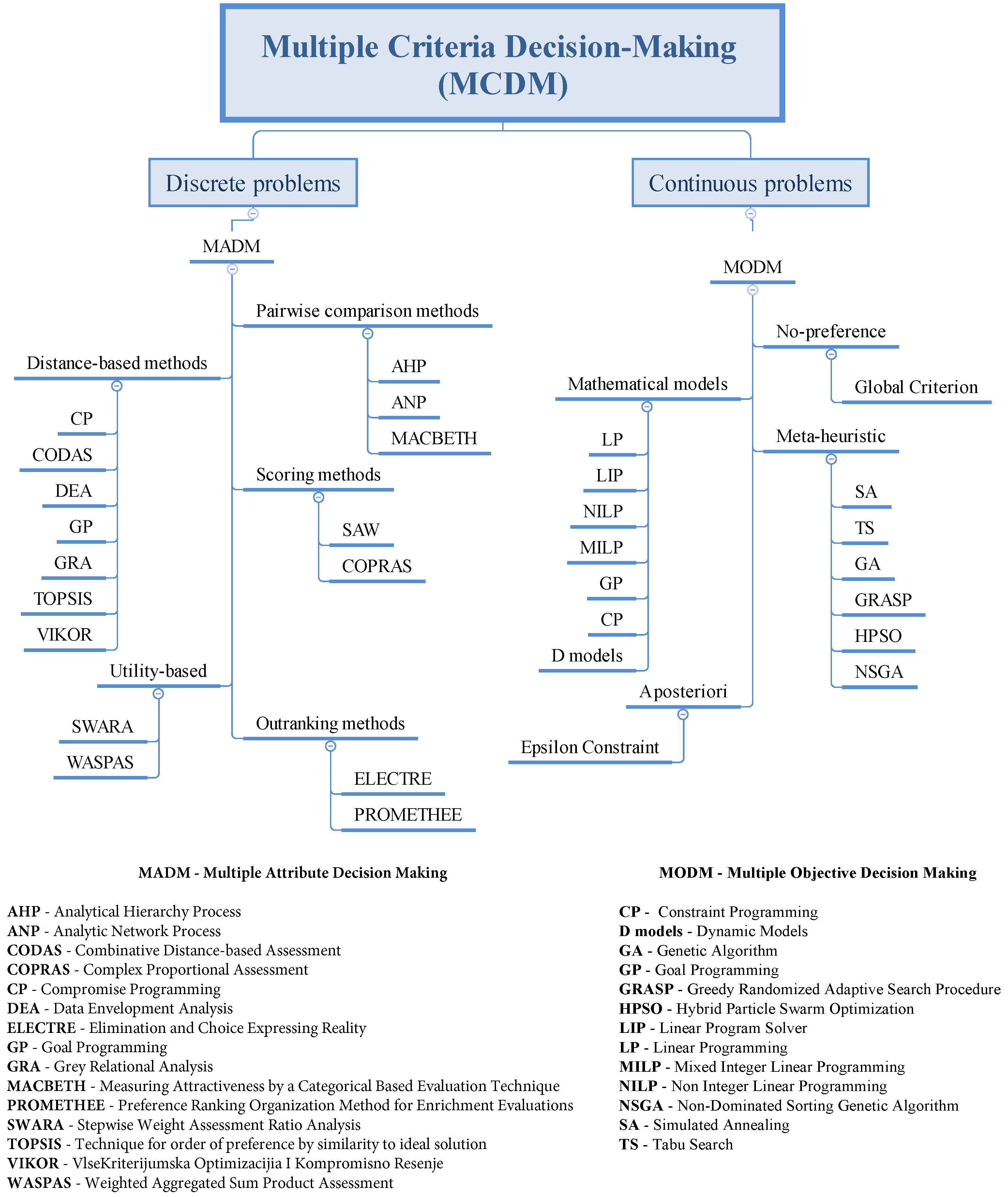
- Multi-Attribute Decision Making (MADM): It is suitable for evaluating discrete decision spaces with predetermined decision alternatives. The MADM approach requires selecting a predetermined and limited number of decision alternatives. In addition to sorting and ranking, MADM approaches can be seen as alternative methods for combining information in a problem’s decision matrix with additional information from the decision maker to determine a final ranking or selection from among the alternatives [36].
- Multi-Objective Decision Making (MODM): It is preferably used for continuous decision problems where the alternatives are not predetermined. Instead of optimizing a goal function, it is focused on optimizing several goal functions.
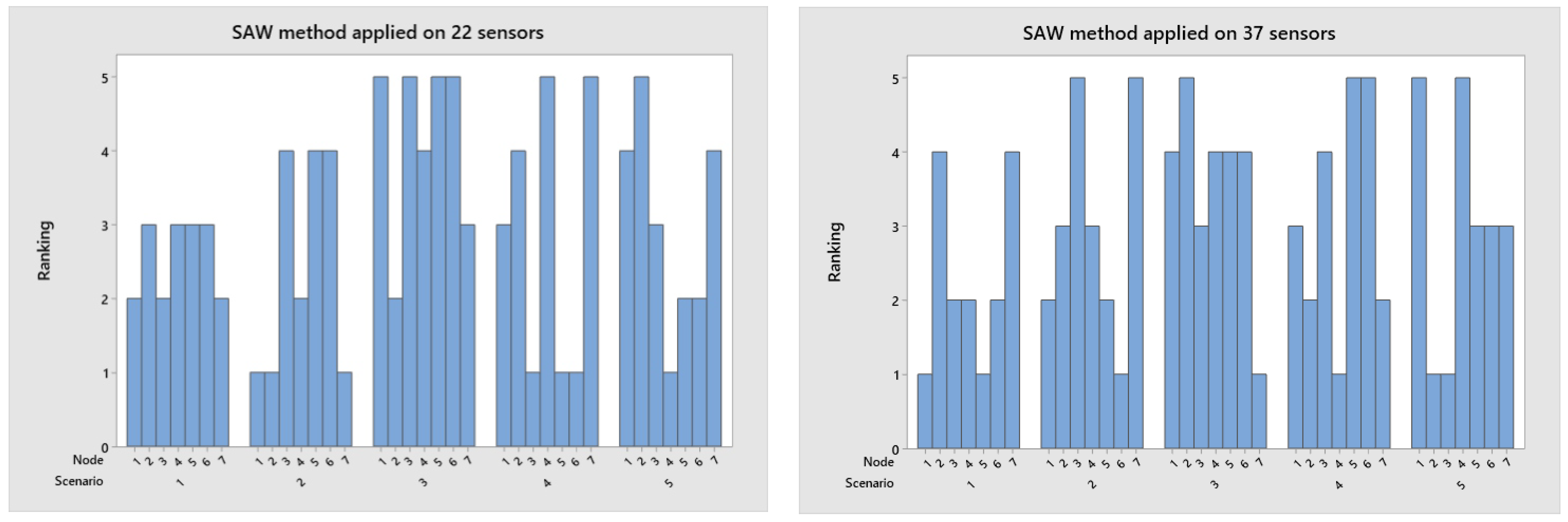
3.1. Simple Additive Weighting (SAW)
- The criteria used as a reference in the decision are specified and named in ();
- It is necessary to determine the adjustment value of each alternative in each attribute;
- Make decisions based on the criteria in the array (). The matrix is normalized according to the fitted equations for the attribute type (attribute or attribute benefit costs) to obtain the normalized matrix;
- The final result is obtained from the multiplication process of the classification matrix, which is the sum of the normalized R with the weight vector. This way, the highest value is obtained and selected as the best alternative () for the solution.
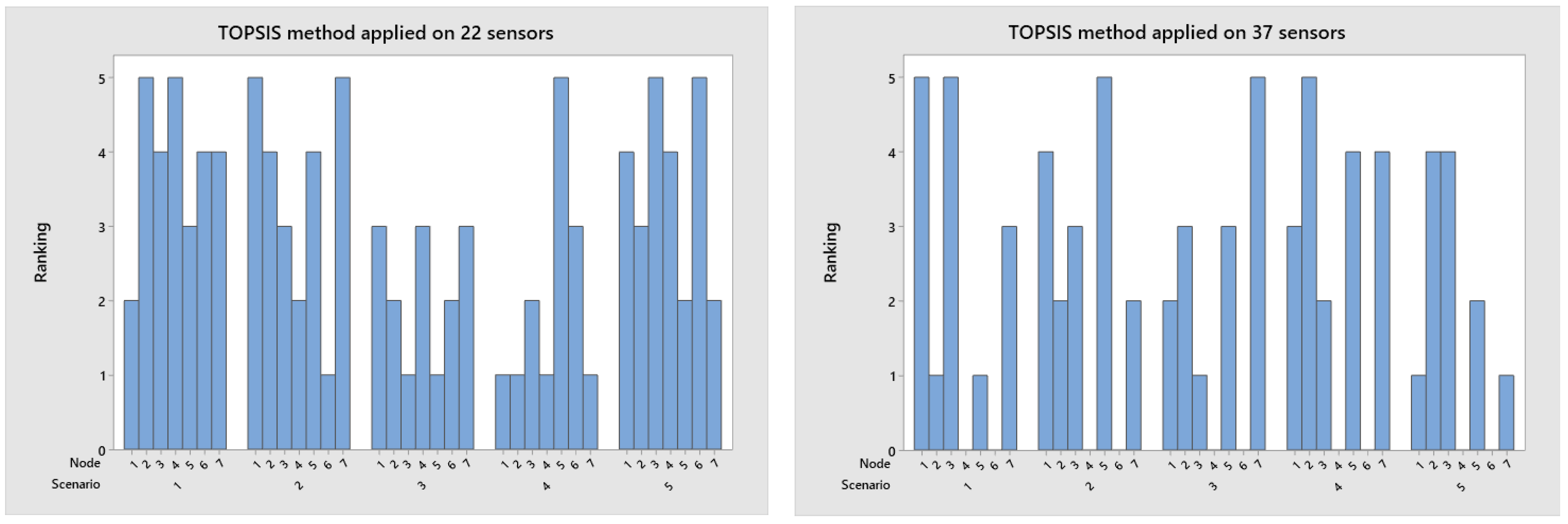
3.2. Technique for the Order of Prioritisation by Similarity to Ideal Solution (TOPSIS)
- The decision matrix D is represented as
- The elements of the ordered decision matrix are calculated according to Equation (4).
- To generate the weighted ordered decision matrix, the corresponding weights of the different criteria are multiplied with the obtained values .
- The PIS and the NIS are formulated according to Equations (5) and (6).where i = 1, 2, 3 …. M e j = 1, 2, 3, …, NJ ∈ {Benefit Criteria Set}∈ {Cost Criteria}
- The distance of each alternative is calculated from the PIS and NIS according to Equations (7) and (8).
- The relative proximity of each alternative is calculated according to Equation (9).Finally, the values of the proximity coefficient obtained with Equation (9) make it possible to calculate the ranking order.
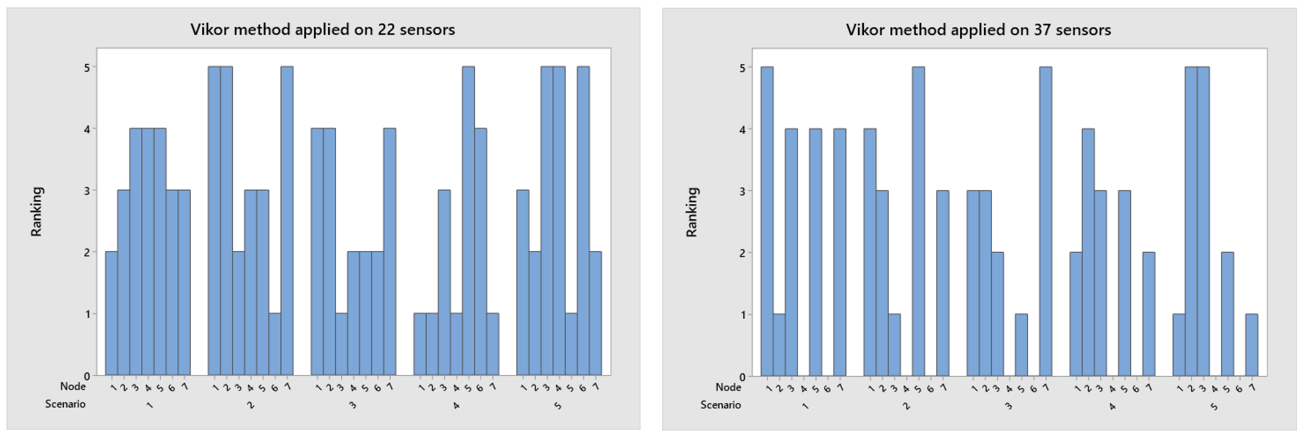
3.3. VIseKriterijumska Optimizacija I Kompromisno Resenje (VIKOR)
- Determines the best and worst values of all functions and criteria, j = 1, 2, …, m. If function j represents a benefit, then or adjust is the desired/desired level, being the worst-level configuration .
- Calculate the values and , k = 1, 2, …, n, by the relations:, displayed as the average distance;, shows how the maximum distance to priority improves, where are the criteria weights.
- Calculates the value , k = 1, 2, …, n, by the relation, k = 1, 2, …, m (alternatives).where:or leave , desired level;or leave , worst level;or leave , desired level;or leave , worst level.Therefore, it is possible to rewrite , when , , and . It is worth mentioning that v is introduced because it is the weight of the “majority of criteria” approach (or “the maximum utility of the group”), here v = 0.5.
- Rank the alternatives, sorted by the values S, R, and Q, in descending order. The result is three ordered lists.
4. Case Study
- All data is collected at runtime during the simulation of the analyzed scenarios;
- All sensors are emulated, so it is possible to carry out simulations with different types of sensors and obtain results closer to the real world;
- The performance analysis of the fog network infrastructure is carried out before its implantation.
- MADM methods are applied to multiple criteria involving different layers of the conceptual communication architecture model.
4.1. Problem Presentation
4.2. Experiment Execution
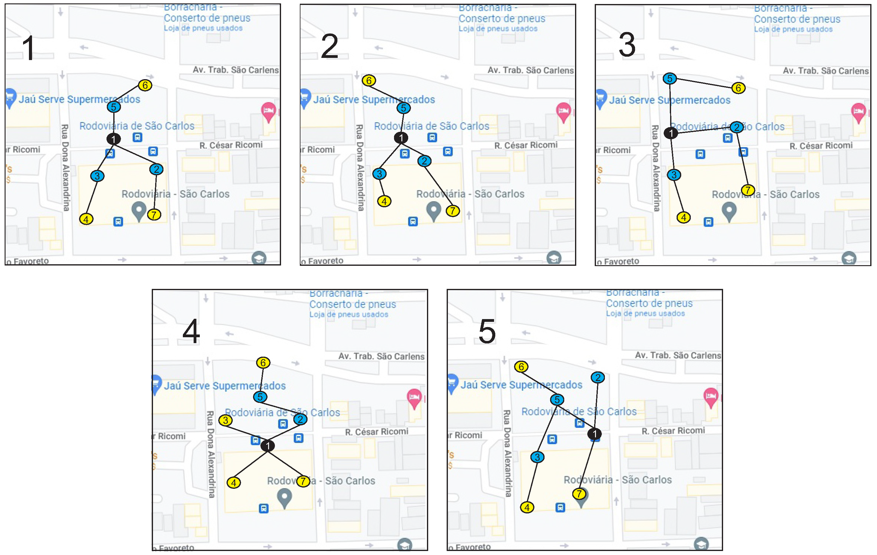
- Alternatives: A set of alternatives will be classified: the five different scenarios presented in Figure 5.
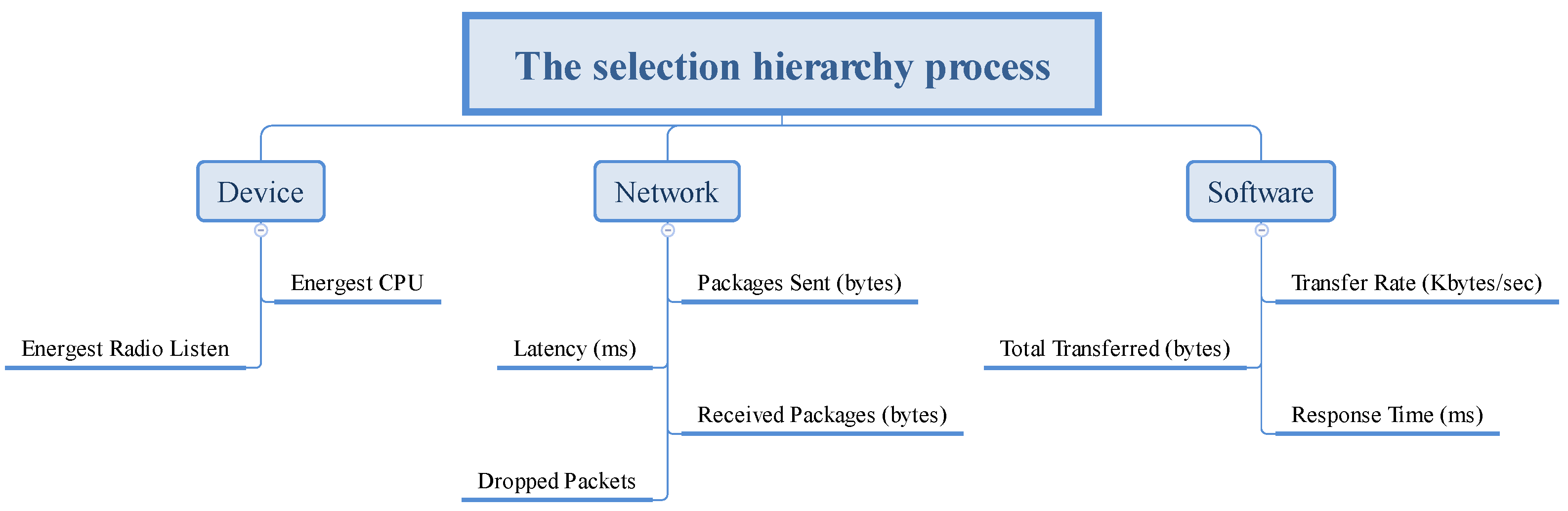
- Attribute set: Represents criteria used in the decision-making process. For each scenario, the sub-criteria are present in Figure 4.
- Weights: The weights for the sub-criteria used in the decision process are shown in Table 3.
5. Results
6. Conclusions
Author Contributions
Funding
Institutional Review Board Statement
Informed Consent Statement
Data Availability Statement
Acknowledgments
Conflicts of Interest
References
- Frei, M.; Deb, C.; Stadler, R.; Nagy, Z.; Schlueter, A. Wireless sensor network for estimating building performance. Autom. Constr. 2020, 3, 1–17. [Google Scholar] [CrossRef]
- Sarkar, S.; Chatterjee, S.; Misra, S. Assessment of the Suitability of Fog Computing in the Context of Internet of Things. IEEE Trans. Cloud Comput. 2018, 6, 46–59. [Google Scholar] [CrossRef]
- Ramirez, W.; Masip-Bruin, X.; Marin-Tordera, E.; Souza, V.B.C.; Jukan, A.; Ren, G.-J.; Dios, O.G. Evaluating the benefits of combined and contínuos Fog-to-Cloud architectures. J. Comput. Commun. 2017, 9, 43–52. [Google Scholar] [CrossRef] [Green Version]
- Salaht, F.A.; Desprez, F.; Lebre, A. An Overview of Service Placement Problem in Fog and Edge Computing. ACM Comput. Surv. 2020, 6, 1–35. [Google Scholar] [CrossRef]
- Andrabi, U.M.; Stepanov, S.N. The model of conjoint servicing of real time traffic of surveillance cameras and elastic traffic devices with access control. Int. Inform. Softw. Eng. Conf. (IISEC) 2021, 12, 1–6. [Google Scholar]
- Agarwal, V.; Tapaswi, S.; Chanak, P. A Survey on Path Planning Techniques for Mobile Sink in IoT-Enabled Wireless Sensor Networks. Wirel. Pers. Commun. 2021, 3, 211–238. [Google Scholar] [CrossRef]
- Gonzalez, O.B.; Chilo, J. WSN IoT Ambient Environmental Monitoring System. In Proceedings of the IEEE 5th International Symposium on Smart and Wireless Systems within the Conferences on Intelligent Data Acquisition and Advanced Computing Systems (IDAACS-SWS), Online, 17–18 September 2020; pp. 1–4. [Google Scholar]
- Rajput, A.; Kumaravelu, V.B. FCM clustering and FLS based CH selection to enhance sustainability of wireless sensor networks for environmental monitoring applications. J. Ambient. Intell. Humaniz. Comput. 2021, 12, 1139–1159. [Google Scholar] [CrossRef]
- Bach, K.H.V.; Kim, S. Towards Evaluation the Cornerstone of Smart City Development: Case Study in Dalat City, Vietnam. Smart Cities 2020, 3, 1–16. [Google Scholar] [CrossRef] [Green Version]
- Astrain, J.J.; Falcone, F.; Lopez, A.; Sanchis, P.; Villadangos, J.; Matias, I.R. Monitoring of Electric Buses within an Urban Smart City Environment. IEEE Sens. 2020, 22, 11364–11372. [Google Scholar] [CrossRef]
- Rizi, M.H.P.; Seno, S.A.H. A systematic review of technologies and solutions to improve security and privacy protection of citizens in the smart city. Internet Things 2022, 20, 100584. [Google Scholar] [CrossRef]
- Chavhan, S.; Gupta, D.; Chandana, B.N.; Khanna, A.; Rodrigues, J.J.P.C. IoT-Based Context-Aware Intelligent Public Transport System in a Metropolitan Area. IEEE Internet Things J. 2020, 11, 6023–6034. [Google Scholar] [CrossRef]
- Phasinam, K.; Kassanuk, T.; Shinde, P.P.; Thakar, C.M.; Sharma, D.K.; Mohiddin, M.K.; Rahmani, A.W. Application of IoT and Cloud Computing in Automation of Agriculture Irrigation. J. Food Qual. 2022, 2022, 8285969. [Google Scholar] [CrossRef]
- Novak, H.; Ratković, M.; Cahun, M.; Lešić, V. An IoT-Based Encapsulated Design System for Rapid Model Identification of Plant Development. Telecom 2022, 3, 70–85. [Google Scholar] [CrossRef]
- Lam, H.F.; Yang, J.H.; Hu, Q. How to Install Sensors for Structural Model Updating? Procedia Eng. 2011, 14, 450–459. [Google Scholar] [CrossRef] [Green Version]
- Al-Fuqaha, A.; Guizani, M.; Mohammadi, M.; Aledhari, M.; Ayyash, M. Internet of things: A survey on enabling technologies, protocols, and applications. IEEE Commun. Surv. Tutorials 2015, 4, 2347–2376. [Google Scholar] [CrossRef]
- Caminha, P.H.C.; Costa, L.H.M.K.; Couto, R.S.; Fladenmuller, A.; Amorim, M.D. On the Coverage of Bus-Based Mobile Sensing. Sensors 2018, 5, 1976. [Google Scholar] [CrossRef] [Green Version]
- Ali, J.; Dyo, V. Coverage and Mobile Sensor Placement for Vehicles on Predetermined Routes: A Greedy Heuristic Approach. In Proceedings of the 2017 14th International Joint Conference on e-Business and Telecommunications (ICETE 2017), Madrid, Spain, 26–28 July 2017; Volume 7, pp. 83–88. [Google Scholar]
- Cruz, P.; Silva, F.F.; Pacheco, R.G.; Couto, R.S.; Velloso, P.B.; Campista, M.E.M.; Costa, L.H.M.K. SensingBus: Using Bus Lines and Fog Computing for Smart-Sensing the City. IEEE Cloud Comput. 2018, 9, 58–69. [Google Scholar] [CrossRef]
- Silva, R.A.C.; Fonseca, N.L.S. On the Location of Fog Nodes in Fog-Cloud Infrastructures. Sensors 2019, 19, 2445. [Google Scholar] [CrossRef] [Green Version]
- Luo, W.; Gu, B.; Lin, G. Communication scheduling in data gathering networks of heterogeneous sensors with data compression: Algorithms and empirical experiments. Eur. J. Oper. Res. 2018, 271, 462–473. [Google Scholar] [CrossRef]
- Nong, S.-X.; Yang, D.-H.; Yi, T.-H. Pareto-Based Bi-Objective Optimization Method of Sensor Placement in Structural Health Monitoring. Buildings 2021, 11, 549. [Google Scholar] [CrossRef]
- Alsaryrah, O.; Mashal, I.; Chung, T.-Y. Bi-Objective Optimization for Energy Aware Internet of Things Service Composition. IEEE Access 2018, 5, 26809–26819. [Google Scholar] [CrossRef]
- Songhorabadi, M.; Rahimi, M.; MoghadamFarid, A.; Kashani, M.H. Fog computing approaches in IoT-enabled smart cities. J. Netw. Comput. Appl. 2023, 211, 103557. [Google Scholar] [CrossRef]
- Nunes, L.H.; Estrella, J.C.; Perera, C.; Reiff-Marganiec, S.; Delbem, A.C.B. Multi-criteria iot resource discovery: A comparative analysis. Softw. Pract. Exp. 2016, 47, 1325–1341. [Google Scholar] [CrossRef] [Green Version]
- Neeraj; Goraya, M.S.; Singh, D. A comparative analysis of prominently used MCDM methods in cloud environment. J. Supercomput. 2021, 77, 3422–3449. [Google Scholar] [CrossRef]
- Ma, Z.; Nejat, M.H.; Vahdat-nejad, H.; Barzegar, B.; Fatehi, S. An Efficient Hybrid Ranking Method for Cloud Computing Services Based on User Requirements. IEEE Access 2022, 6, 72988–73004. [Google Scholar] [CrossRef]
- Youssef, A.E. An Integrated MCDM Approach for Cloud Service Selection Based on TOPSIS and BWM. IEEE Access 2020, 8, 71851–71865. [Google Scholar] [CrossRef]
- Mashal, I.; Alsaryrah, O.; Chung, T.; Yuan, F. A multi-criteria analysis for an internet of things application recommendation system. Technol. Soc. 2020, 60, 101216. [Google Scholar] [CrossRef]
- Kadhim, M.H.; Mardukhi, F. A Novel IoT Application Recommendation System Using Metaheuristic Multi-Criteria Analysis. Comput. Syst. Sci. Eng. 2021, 37, 149–158. [Google Scholar]
- Jiang, F.; Feng, C.; Zhang, H. A heterogenous network selection algorithm for internet of vehicles based on comprehensive weight. Alex. Eng. J. 2021, 5, 4677–4688. [Google Scholar] [CrossRef]
- Ahmad, M.; Ahmad, M.; Khurshid, F.; Hu, J.; Zaid-ul-Huda. Optimal Cluster Leader Selection Using MCDM Methods in MWSN: A Comparative Study. In Proceedings of the 2019 IEEE 14th International Conference on Intelligent Systems and Knowledge Engineering (ISKE), Dalian, China, 14–16 November 2019; pp. 240–247. [Google Scholar]
- Gómez, D.; Martínez, J.-F.; Sendra, J.; Rubio, G. Development of a Decision Making Algorithm for Traffic Jams Reduction Applied to Intelligent Transportation Systems. J. Sens. 2016, 2016, 9271986. [Google Scholar] [CrossRef] [Green Version]
- Bendaoud, F.; Abdennebi, M.; Didi, F. Network Selection in Wireless Heterogeneous Networks: A Survey. J. Telecommun. Inf. Technol. 2019, 4, 64–74. [Google Scholar] [CrossRef]
- Hwang, C.-L.; Yoon, K. Methods for multiple attribute decision making. In Multiple Attribute Decision Making; Springer: Berlin/Heidelberg, Germany, 1981; pp. 58–191. [Google Scholar]
- Devi, K.; Yadav, S.P.; Kumar, S. Extension of Fuzzy TOPSIS Method Based on Vague Sets. Int. J. Comput. Cogn. 2009, 7, 58–62. [Google Scholar]
- Ogundoyin, S.O.; Kamil, I.A. Optimization techniques and applications in fog computing: An exhaustive survey. Swarm Evol. Comput. 2021, 6, 100937. [Google Scholar] [CrossRef]
- Muslihudin, M.; Trisnawati, A.; Latif, R.; Wati, A.; Maseleno, A. Optimization techniques and applications in fog computing: An exhaustive survey. Int. J. Pure Appl. Math. 2018, 66, 261–267. [Google Scholar]
- Sahir, S.H.; Rosmawati, R.; Minan, K. Simple Additive Weighting Method to Determining Employee Salary Increase Rate. Int. J. Sci. Res. Sci. Technol. (IJSRST) 2017, 3, 42–48. [Google Scholar]
- Muslihudin, M.; Gumati, M. A System To Support Decision Makings In Selection Of Aid Receivers For Classroom Rehabilitation For Senior High Schools By Education Office Of Pringsewu District By. IJISCS (Int. J. Inf. Syst. Comput. Sci.) 2017, 1, 1–9. [Google Scholar]
- Fauzi; Nungsiyati; Noviarti, T.; Muslihudin, M.; Irviani, R.; Maseleno, A. Optimal Dengue Endemic Region Prediction using Fuzzy Simple Additive Weighting based Algorithm. Int. J. Pure Appl. Math. 2018, 118, 473–478. [Google Scholar]
- Hwang, C.-L.; Yoon, K. Multiple Attribute Decision Making Methods and Applications A State-of-the-Art Survey; Springer: Berlin/Heidelberg, Germany, 1981; Volume 86. [Google Scholar]
- Abidin, M.Z.; Rusli, R.; Shariff, A.M. Technique for Order Performance by Similarity to Ideal Solution (TOPSIS)-entropy Methodology for Inherent Safety Design Decision Making Tool. In Proceedings of the 4th International Conference on Process Engineering and Advanced Materials, Kuala Lumpur, Malaysia, 15–17 August 2016; pp. 1043–1050. [Google Scholar]
- Li, X.; Han, Y.; Wu, X.; Zhang, D.A. Evaluating node importance in complex networks based on TOPSIS and gray correlation. In Proceedings of the 2018 Chinese Control And Decision Conference (CCDC), Shenyang, China, 9–11 June 2018; pp. 750–754. [Google Scholar]
- Dong, C.; Xu, G.; Meng, L.; Yang, P. CPR-TOPSIS: A novel algorithm for finding influential nodes in complex networks based on communication probability and relative entropy. Physica A 2022, 603, 127797. [Google Scholar] [CrossRef]
- Ashraf, Q.M.; Habaebi, M.H.; Islam, M.R. TOPSIS-Based Service Arbitration for Autonomic Internet of Things. IEEE Access 2016, 4, 1313–1320. [Google Scholar] [CrossRef]
- Alhalameh, A.R.; Al-Tarawneh, M.A.B. Integrated Multi-Criteria Decision Making Approach for Service Brokering in Cloud-enabled IoT Environments. In Proceedings of the International Conference on Emerging Trends in Computing and Engineering Applications (ETCEA), Karak, Jordan, 23–25 November 2022; pp. 1–5. [Google Scholar]
- Sahraneshin, T.; Malekhosseini, R.; Rad, F.; Yaghoubyan, S.H. Securing communications between things against wormhole attacks using TOPSIS decision-making and hash-based cryptography techniques in the IoT ecosystem. Wirel. Netw. 2022, 29, 1–15. [Google Scholar] [CrossRef]
- Zheng, F.; Lin, Y. A Fuzzy TOPSIS expert system based on neural networks for new product design. In Proceedings of the 2017 International Conference on Applied System Innovation (ICASI), Sapporo, Japan, 13–17 May 2017; pp. 598–601. [Google Scholar]
- Huang, H. Research on Raw Material Ordering and Transportation Process Based on TOPSIS and Neural Network. In Proceedings of the 2nd International Conference on Computer Engineering and Intelligent Control (ICCEIC), Chongqing, China, 12–14 November 2021; pp. 68–72. [Google Scholar]
- Anandavelu, T.; Rajkumar, S.; Thangarasu, V. Dual fuel combustion of 1-hexanol with diesel and biodiesel fuels in a diesel engine: An experimental investigation and multi criteria optimization using artificial neural network and TOPSIS algorithm. Fuel 2023, 338, 127318. [Google Scholar] [CrossRef]
- Jain, V.; Khan, S.A. Reverse logistics service provider selection: A TOPSIS-QFD approach. In Proceedings of the 2016 IEEE International Conference on Industrial Engineering and Engineering Management (IEEM), Bali, Indonesia, 4–7 December 2016; pp. 803–806. [Google Scholar]
- Badulescu, Y.; Tiwari, M.K.; Cheikhrouhou, N. MCDM approach to select IoT devices for the reverse logistics process in the Clinical Trials supply chain. IFAC-PapersOnLine 2022, 55, 43–48. [Google Scholar] [CrossRef]
- Nunes, L.H.; Estrella, J.C.; Nakamura, L.H.V.; Libardi, R.; Ferreira, C.H.G.; Jorge, L.; Perera, C.; Reiff-Marganiec, S. A Distributed Sensor Data Search Platform for Internet of Things Environments. Int. J. Serv. Comput. 2016, 4, 1–12. [Google Scholar]
- Jin, G.; Jin, G. Fault-Diagnosis Sensor Selection for Fuel Cell Stack Systems Combining an Analytic Hierarchy Process with the Technique Order Performance Similarity Ideal Solution Method. Symmetry 2021, 13, 2366. [Google Scholar] [CrossRef]
- Bouarourou, S.; Boulaalam, A.; Nfaoui, E.H. A bio-inspired adaptive model for search and selection in the Internet of Things environment. PeerJ Comput. Sci. 2021, 7, e762. [Google Scholar] [CrossRef] [PubMed]
- Panda, M.; Jagadev, A.K. TOPSIS in Multi-Criteria Decision Making: A Survey. In Proceedings of the 2018 2nd International Conference on Data Science and BUSINESS Analytics (ICDSBA), Changsha, China, 21–23 September 2018; pp. 51–54. [Google Scholar]
- Opricovic, S.; Tzeng, G. Compromise solution by MCDM methods: A comparative analysis of VIKOR and TOPSIS. Eur. J. Oper. Res. 2004, 156, 445–455. [Google Scholar] [CrossRef]
- Mardani, A.; Zavadskas, E.K.; Govindan, K.; Senin, A.A.; Jusoh, A. VIKOR Technique: A Systematic Review of the State of the Art Literature on Methodologies and Applications. Sustainability 2016, 8, 37. [Google Scholar] [CrossRef] [Green Version]
- Verba, N.; Chao, K.; James, A.E.; Goldsmith, D.J.; Fei, X. Platform as a Service Gateway for the Fog of Things. Adv. Eng. Inform. 2017, 33, 243–257. [Google Scholar] [CrossRef] [Green Version]
- Veeramani, S.; Mahammad, S.N. An Approach to Place Sink Node in a Wireless Sensor Network (WSN). Wirel. Pers. Commun. 2020, 111, 1117–1127. [Google Scholar] [CrossRef]
- Bendigeri, K.Y.; Mallapur, J.D.; Kumbalavati, S.B. Direction Based Node Placement in Wireless Sensor Network. In Proceedings of the International Conference on Artificial Intelligence and Smart Systems (ICAIS), Coimbatore, India, 25–27 March 2021; pp. 1306–1313. [Google Scholar]
- Taherdoost, H.; Madanchian, M. Multi-Criteria Decision Making (MCDM) Methods and Concepts. Encyclopedia 2023, 3, 77–87. [Google Scholar] [CrossRef]


| Reference | Technique/Method | Algorithms | Main Criterion | Metric/Parameters of Evaluation | Application Areas | Year |
|---|---|---|---|---|---|---|
| [27] | Software based approach | AHP Fuzzy AHP | Accountability | - | Cloud Service | 2022 |
| Capacity | ||||||
| Elasticity | ||||||
| Agility | Transparency | |||||
| Availability | ||||||
| Interoperability | ||||||
| Service Stability | ||||||
| Serviceability | ||||||
| Assurance | Reliability | |||||
| Cost | Service Cost | |||||
| Service Response Time | ||||||
| Throughput | ||||||
| Performance | Accuracy | |||||
| Security | - | |||||
| [26] | Software based approach | AHP PROMETHEE II TOPSIS VIKOR | Quality of Service (QoS) | Services | Cloud Service | 2021 |
| Availability zone | ||||||
| Distance | ||||||
| Cost | ||||||
| [30] | Software based approach | SQL Programming SAW ANP | Cost | IoT Applications | 2021 | |
| Energy Consumption | ||||||
| Smart Objects | Installation | |||||
| Interoperability | ||||||
| Availability | ||||||
| Ease of Use | ||||||
| Application | Interface | |||||
| Privacy | ||||||
| Reliability | ||||||
| Customer Care | ||||||
| Provider | Reputation | |||||
| Number of Customers | ||||||
| Proposed work | Hardware and Software based approach | SAW TOPSIS VIKOR | Energest CPU | Fog Service | 2023 | |
| Device | Energest radio listen | |||||
| Packets sent | ||||||
| Packets received | ||||||
| Latency | ||||||
| Network | Lost packets | |||||
| Response time | ||||||
| Transfer rate | ||||||
| Software | Total transferred | |||||
| [28] | Software based approach | AHP Hybrid (TOPSIS & Best-Worst Method) | Sustainability | Cloud Service | 2020 | |
| Interoperability | ||||||
| Performance | Service response time | |||||
| Maintainability | ||||||
| Assurance | Reliability | |||||
| Financial | Cost | |||||
| Security & Privacy | Security Management | |||||
| Agility | Scalability | |||||
| Usuability | Usuability | |||||
| [25] | Software based approach | SAW VIKOR TOPSIS Pareto Optimal | Smart Objects | Battery | IoT Devices | 2016 |
| Price | ||||||
| Drift | ||||||
| Frequency | ||||||
| Energy Consumption | ||||||
| Response Time | ||||||
| [29] | Software based approach | AHP SAW | Cost | IoT Applications | 2020 | |
| Energy Consumption | ||||||
| Smart Objects | Installation | |||||
| Interoperability | ||||||
| Availability | ||||||
| Ease of Use | ||||||
| Application | Interface | |||||
| Privacy | ||||||
| Reliability | ||||||
| Customer Care | ||||||
| Provider | Reputation | |||||
| Number of Customers | ||||||
| [31] | Software based approach | AHP | Delay | Heterogenous Network | 2021 | |
| Packet loss rate | ||||||
| QoS | Bandwith | |||||
| Jitter | ||||||
| Available load | ||||||
| Cost | ||||||
| [32] | Software based approach | Fuzzy TOPSIS Fuzzy AHP | Cluster leader | Link Reliabililty | Cluster Leader Selection | 2019 |
| Connectivity | ||||||
| Remaining Energy | ||||||
| Distance to BS | ||||||
| Speed | ||||||
| [34] | Survey | SAW TOPSIS Weighted Product Model AHP GRA | Throughput | Network Selection | 2019 | |
| Delay | ||||||
| Application | Jitter | |||||
| PLR | ||||||
| Energy consumption | ||||||
| Network load | ||||||
| Network coverage | ||||||
| Network | Network connection time | |||||
| Available bandwidth | ||||||
| Battery level | ||||||
| Device | Mobility | |||||
| Budget | ||||||
| User preferences | Cost | |||||
| [33] | Software based approach | Fuzzy AHP Dynamic AHP | Congestion control | Traffic flow | Intelligent Transportation Systems | 2016 |
| Average speed | ||||||
| Occupancy rate |
| Parameters | Value |
|---|---|
| Simulation Tool | Contiki-NG |
| MAC | CSMA/CA |
| Transport | UDP/IPv6 |
| Deployment type | Mobile and static position |
| Emulated nodes | Cooja |
| Simulation coverage area | 1000 m × 1000 m |
| Total number of sensors | 22–37 |
| Fog Nodes | 7 |
| Sink Node | 1 |
| RX/TX ratio | 100% |
| TX range | 50 m |
| Interference range | 100 m |
| Packet size | 64 byte |
| Routing protocols | RPL Lite |
| Network protocol | IP based |
| Link failure model | UDGM with distance |
| Simulation time | 60 min |
| Alternatives | Packets Send (bytes) | Latency (ms) | Packets Received (bytes) | Energest CPU | Packages Dropped | Energest Radio Listen (seconds) | Total Transferred (bytes) | Transfer Rate (Kbytes/sec) | Total Time (ms) | |
|---|---|---|---|---|---|---|---|---|---|---|
| 1 | 1 | 1151.6974 | 2294.9027 | 720.2119 | 1181.3946 | 0 | 74.9270 | 1823.4126 | 2.37 | 973.6 |
| 2 | 375.7328 | 837.1118 | 473.1630 | 1187.8366 | 154 | 94.0973 | 237.5 | 0.11 | 4077.0727 | |
| 3 | 453.7193 | 1420.8156 | 552.4587 | 1187.1963 | 102 | 62.3146 | 238.0350 | 0.12 | 3936.5087 | |
| 4 | 215.5718 | 2003.5093 | 338.4059 | 1187.8366 | 345 | 145.7097 | 238.9423 | 0.03 | 14,211.7115 | |
| 5 | 432.9369 | 1515.3815 | 672.5302 | 1187.1963 | 6 | 56.2967 | 238.5535 | 0.13 | 4568.7321 | |
| 6 | 143.1311 | 1703.5139 | 218.7788 | 1187.8366 | 465 | 286.1891 | 239.4893 | 0.03 | 13,469.2340 | |
| 7 | 192.7308 | 2417.8158 | 296.8264 | 1187.8366 | 492 | 234.4047 | 239.6458 | 0.04 | 9813.0833 | |
| 2 | 1 | 784.8094 | 2700.8251 | 487.9957 | 1082.0630 | 0 | 80.0212 | 1745.05454 | 1.78 | 1303.6 |
| 2 | 226.2675 | 775.2763 | 264.6136 | 881.9036 | 18 | 53.9772 | 237.3 | 0.09 | 6020.2040 | |
| 3 | 510.7335 | 1357.9500 | 738.5428 | 882.33 | 106 | 79.3064 | 237.3695 | 0.11 | 4836.6739 | |
| 4 | 425.4716 | 2358.2422 | 698.2689 | 881.4670 | 76 | 118.6232 | 238.3953 | 0.02 | 17,349.5116 | |
| 5 | 253.7624 | 1049.4834 | 365.2913 | 881.1107 | 11 | 39.5167 | 237.6382 | 0.10 | 5232.2553 | |
| 6 | 154.1110 | 1578.6963 | 256.8010 | 879.3961 | 213 | 163.6175 | 238.8780 | 0.34 | 12,609.1463 | |
| 7 | 193.4476 | 2770.4797 | 318.7458 | 880.6006 | 256 | 152.5918 | 239.4102 | 0.03 | 19,391.6153 | |
| 3 | 1 | 815.7785 | 2027.7524 | 500.8345 | 1246.3380 | 0 | 81.2630 | 1507.1166 | 2.55 | 658.2 |
| 2 | 242.4766 | 1057.9882 | 289.9858 | 983.6701 | 0 | 51.5223 | 237.36 | 0.13 | 4646.4166 | |
| 3 | 347.3028 | 573.6886 | 400.6295 | 980.2740 | 0 | 36.6937 | 237.3333 | 0.15 | 2377.55 | |
| 4 | 117.8570 | 1957.6918 | 175.8373 | 953.0230 | 150 | 204.4628 | 239.4629 | 0.03 | 13,678.4444 | |
| 5 | 207.0744 | 667.3410 | 250.5757 | 1205.8702 | 0 | 37.2002 | 238.0344 | 0.14 | 2314.1896 | |
| 6 | 69.2964 | 1281.9875 | 104.0158 | 825.0438 | 139 | 182.1667 | 239.4905 | 0.03 | 10,657.5471 | |
| 7 | 140.7515 | 1718.0373 | 194.8677 | 790.0630 | 59 | 144.9888 | 239.2307 | 0.04 | 8596.9038 | |
| 4 | 1 | 1465.2343 | 1410.2481 | 950.0392 | 1036.1140 | 0 | 90.3310 | 1810.45 | 2.52 | 717.5 |
| 2 | 656.2387 | 764.3295 | 760.3923 | 1500.5576 | 6 | 92.3922 | 238.6800 | 0.14 | 2905.3684 | |
| 3 | 115.0719 | 650.2629 | 235.8162 | 1498.0567 | 0 | 62.8411 | 238.3448 | 0.15 | 2387.9827 | |
| 4 | 169.2818 | 740.2151 | 309.2612 | 1500.2273 | 2 | 87.0167 | 238.8596 | 0.11 | 4459.3684 | |
| 5 | 442.1057 | 1374.8193 | 534.3376 | 1545.5106 | 50 | 191.2584 | 239.8571 | 0.04 | 10,562 | |
| 6 | 175.0576 | 2292.8258 | 243.5753 | 1470.1182 | 298 | 368.7203 | 240.3962 | 0.02 | 20,272.9245 | |
| 7 | 167.1240 | 682.0284 | 298.2276 | 1520.906 | 2 | 93.6152 | 239.1250 | 0.15 | 2397.1964 | |
| 5 | 1 | 785.4181 | 2270.7470 | 516.2583 | 1011.5442 | 0 | 89.6200 | 1832.4705 | 2.78 | 649.0 |
| 2 | 63.7844 | 574.7394 | 112.5267 | 1052.1204 | 35 | 106.4600 | 238.25 | 0.15 | 3529.8958 | |
| 3 | 312.0038 | 2171.7712 | 381.2423 | 1040.6720 | 43 | 105.2626 | 238.7021 | 0.04 | 11,305.9787 | |
| 4 | 509.1450 | 3989.6861 | 932.4428 | 948.5080 | 83 | 168.8371 | 239.3709 | 0.02 | 23,748.3953 | |
| 5 | 550.9463 | 778.4576 | 619.0974 | 1302.0674 | 0 | 35.7709 | 238.0851 | 0.12 | 5945.7446 | |
| 6 | 67.2146 | 2202.9649 | 102.6245 | 1107.3020 | 583 | 314.5345 | 239.5 | 0.03 | 13,444.9166 | |
| 7 | 142.4695 | 741.2840 | 200.3583 | 920.2502 | 15 | 71.0000 | 239.0697 | 0.13 | 3168.8604 | |
| Weights | 0.1 | 0.18 | 0.1 | 0.08 | 0.12 | 0.07 | 0.06 | 0.14 | 0.15 | |
| Alternatives | SAW | VIKOR | TOPSIS | |
|---|---|---|---|---|
| 1 | 1 | 1276.73 | 0.57079 | 0.460932 |
| 2 | 989.37 | 1.00000 | 0.380069 | |
| 3 | 1200.24 | 0.70704 | 0.553937 | |
| 4 | 2679.43 | 0.00000 | 0.351706 | |
| 5 | 1171.98 | 0.67591 | 0.580214 | |
| 6 | 2529.96 | 0.37609 | 0.371579 | |
| 7 | 2098.98 | 1.00000 | 0.392042 | |
| 2 | 1 | 1299.99 | 0.93492 | 0.048142 |
| 2 | 1187.52 | 0.00000 | 0.499016 | |
| 3 | 802.67 | 0.08834 | 0.570139 | |
| 4 | 3200.01 | 0.25635 | 0.507123 | |
| 5 | 1121.16 | 0.18316 | 0.523249 | |
| 6 | 2319.02 | 0.03509 | 0.764470 | |
| 7 | 3528.51 | 0.20060 | 0.283881 | |
| 3 | 1 | 1019.96 | 1.00000 | 0.406849 |
| 2 | 1027.81 | 0.50000 | 0.544202 | |
| 3 | 699.24 | 0.23128 | 0.736800 | |
| 4 | 2524.19 | 0.08939 | 0.444361 | |
| 5 | 610.53 | 0.00000 | 0.619824 | |
| 6 | 1954.33 | 0.60163 | 0.437688 | |
| 7 | 1715.13 | 0.70929 | 0.580576 | |
| 4 | 1 | 1124.54 | 0.34526 | 0.943643 |
| 2 | 875.89 | 0.11585 | 0.826560 | |
| 3 | 1957.23 | 1.00000 | 0.665273 | |
| 4 | 1010.65 | 0.00000 | 0.673957 | |
| 5 | 2086.34 | 0.23784 | 0.361465 | |
| 6 | 3667.49 | 0.03955 | 0.375321 | |
| 7 | 691.96 | 0.22109 | 0.773653 | |
| 5 | 1 | 1108.90 | 0.82969 | 0.379600 |
| 2 | 761.31 | 0.87720 | 0.506544 | |
| 3 | 897.05 | 0.48848 | 0.326897 | |
| 4 | 4443.99 | 0.96344 | 0.435437 | |
| 5 | 1243.03 | 0.50000 | 0.611787 | |
| 6 | 2567.87 | 0.00000 | 0.279571 | |
| 7 | 743.32 | 0.19365 | 0.744092 | |
Disclaimer/Publisher’s Note: The statements, opinions and data contained in all publications are solely those of the individual author(s) and contributor(s) and not of MDPI and/or the editor(s). MDPI and/or the editor(s) disclaim responsibility for any injury to people or property resulting from any ideas, methods, instructions or products referred to in the content. |
© 2023 by the authors. Licensee MDPI, Basel, Switzerland. This article is an open access article distributed under the terms and conditions of the Creative Commons Attribution (CC BY) license (https://creativecommons.org/licenses/by/4.0/).
Share and Cite
Ferreira, A.M.A.; Azevedo, L.J.d.M.d.; Estrella, J.C.; Delbem, A.C.B. Case Studies with the Contiki-NG Simulator to Design Strategies for Sensors’ Communication Optimization in an IoT-Fog Ecosystem. Sensors 2023, 23, 2300. https://0-doi-org.brum.beds.ac.uk/10.3390/s23042300
Ferreira AMA, Azevedo LJdMd, Estrella JC, Delbem ACB. Case Studies with the Contiki-NG Simulator to Design Strategies for Sensors’ Communication Optimization in an IoT-Fog Ecosystem. Sensors. 2023; 23(4):2300. https://0-doi-org.brum.beds.ac.uk/10.3390/s23042300
Chicago/Turabian StyleFerreira, Antonio Marcos Almeida, Leonildo José de Melo de Azevedo, Júlio Cezar Estrella, and Alexandre Cláudio Botazzo Delbem. 2023. "Case Studies with the Contiki-NG Simulator to Design Strategies for Sensors’ Communication Optimization in an IoT-Fog Ecosystem" Sensors 23, no. 4: 2300. https://0-doi-org.brum.beds.ac.uk/10.3390/s23042300