Author Contributions
Conceptualization, Y.Z. (Yingtong Zhou); methodology, Y.Z. (Yingtong Zhou) and T.H.; software, Q.N.; validation, Y.Z. (Yingtong Zhou); formal analysis, Y.Z. (Yingtong Zhou); investigation, Y.Z. (Yingtong Zhou) and T.H.; resources, T.H. and Q.N.; writing—original draft preparation, Y.Z. (Yingtong Zhou); writing—review and editing, Y.Z. (Yingtong Zhou), T.H., Z.L. and Y.Z. (Yuxuan Zhu); visualization, Y.Z. (Yingtong Zhou) and T.H.; supervision, T.H., Q.N. and Z.L.; project administration, Y.Z. (Yuxuan Zhu), M.L., N.B. and Z.L.; funding acquisition, Y.Z. (Yuxuan Zhu), M.L., N.B. and Z.L. All authors have read and agreed to the published version of the manuscript.
Figure 2.
Typical sensor calibration methods involve projecting 3D point clouds onto 2D images to identify features. However, our proposed method establishes data correlation based on pose instead of features. This involves triangulating point and line features on the image plane using pose information and adjusting feature positions and external parameters to minimize reprojection error. Then, we achieve calibrated external parameters.
Figure 3.
We employ two parallel methods for processing point and line features. For point feature processing, we use the SuperPoint algorithm in conjunction with SuperGlue, uniform sampling of points, and optical flow. To extract line features, we make use of the AG3line method and fine-tune it using an expanded photometric error approach. Tracking of the same feature point between frames is shown using arrows and same color point features.
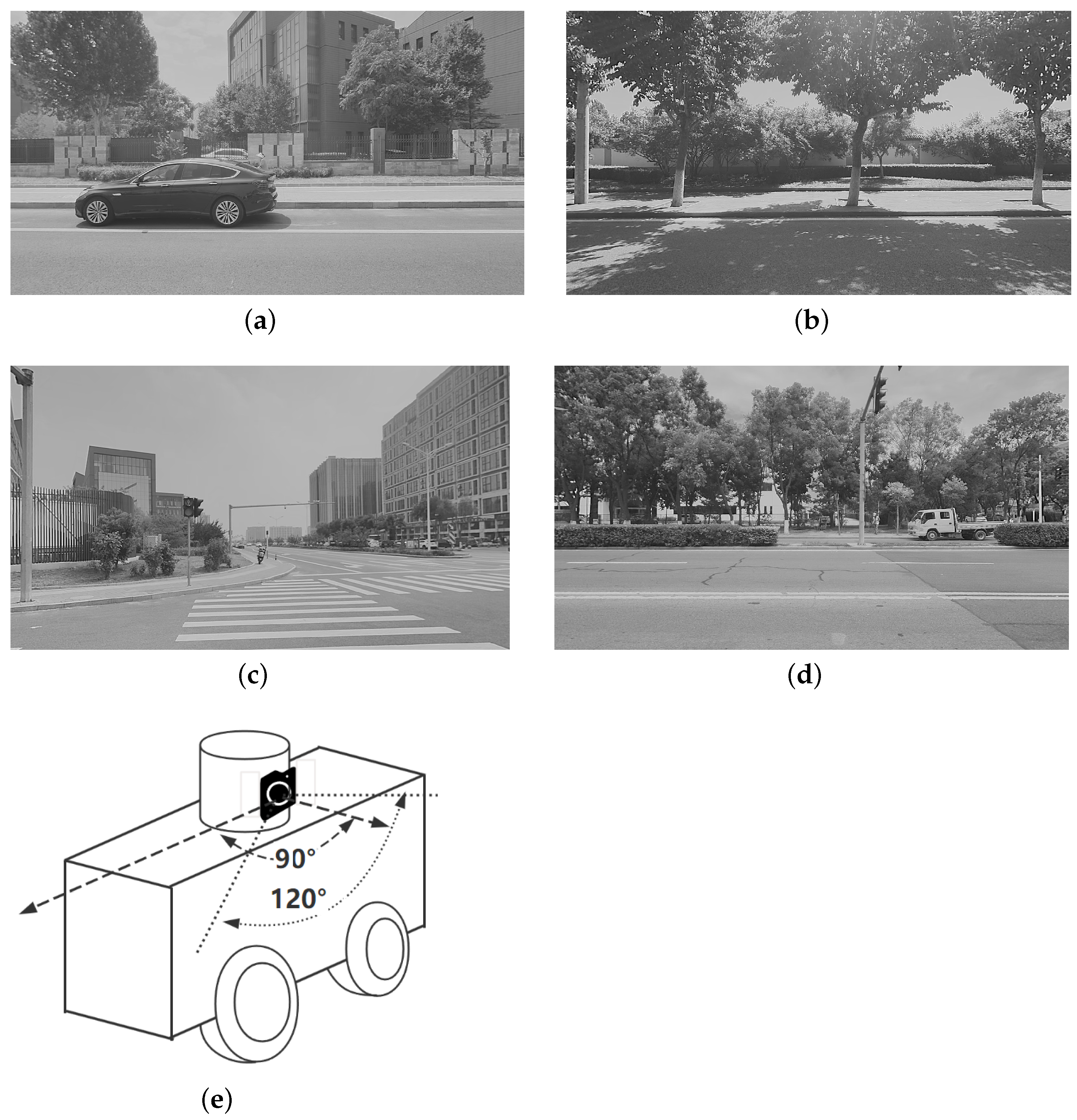
Figure 4.
Our dataset includes various urban scenarios with different lighting conditions, environmental textures, and distances. (a,c): Urban scenarios with less shadow and occlusion or rich environmental textures. (b,d): Urban scenarios with severe shadow and occlusion or unclear environmental features. (e): For our study, we used a side camera, which is fixed above the vehicle’s body. The camera is positioned at 90-degree angle from the center of the vehicle’s body towards its front.
Figure 5.
The figures above show the results obtained after extracting and fine-tuning line features. (a) demonstrates that AG3line can effectively extract scene line features that are clear, coherent, and with very few stray lines. In (b), the results of line feature optimization using the extended photometric error are displayed. The red lines represent the original lines with deviations, while the blue lines represent their positions after fine-tuning. The optimal position is situated closer to the edge.
Figure 6.
Results obtained from the four calibration methods under different extrinsic parameter errors for Sequence 1 are presented. The feature point method has a significant advantage in scenes with sufficient illumination and clear textures.
Figure 6.
Results obtained from the four calibration methods under different extrinsic parameter errors for Sequence 1 are presented. The feature point method has a significant advantage in scenes with sufficient illumination and clear textures.
Figure 7.
Results obtained from the four calibration methods for Sequence 2 are presented under different extrinsic parameter errors. The direct method outperforms the other methods in scenes with weak illumination and unclear textures.
Figure 7.
Results obtained from the four calibration methods for Sequence 2 are presented under different extrinsic parameter errors. The direct method outperforms the other methods in scenes with weak illumination and unclear textures.
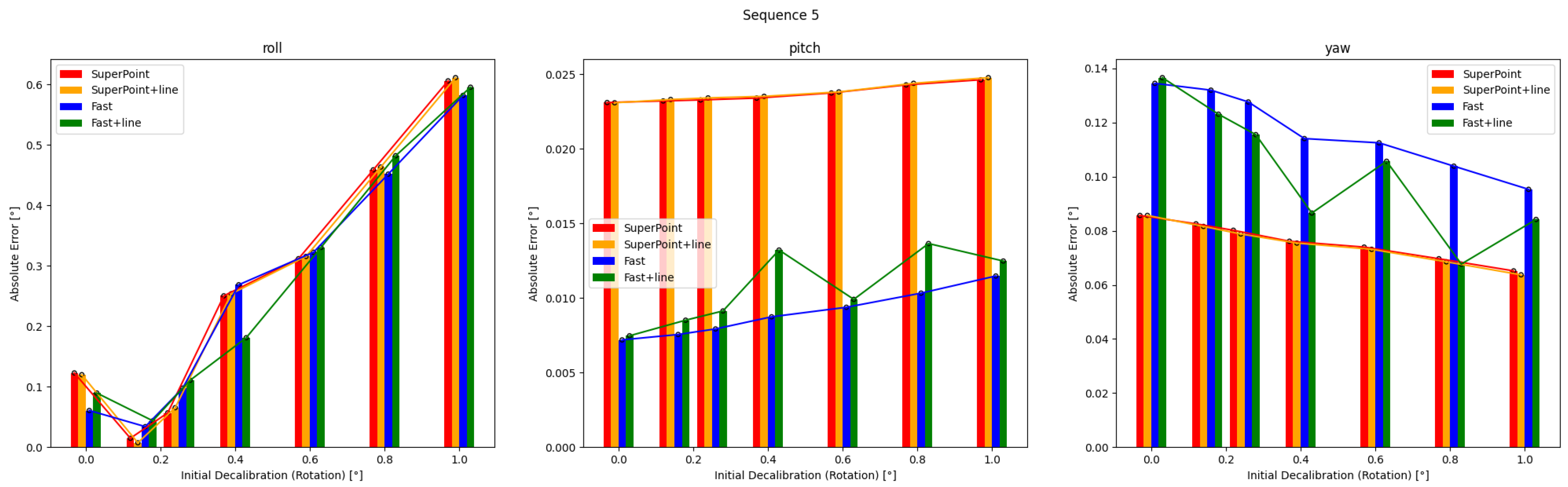
Figure 8.
Results obtained from four calibration methods are presented for Sequence 5 under varying extrinsic parameter errors. Calibration result may change with initial values in more complex mixed scenes.
Figure 8.
Results obtained from four calibration methods are presented for Sequence 5 under varying extrinsic parameter errors. Calibration result may change with initial values in more complex mixed scenes.
Figure 9.
In Sequence 1, during the pre-optimization process, the confidence curves of the two feature methods displayed a clear separation, indicating a significant difference in their effects. Our adaptive selection method chose the SuperPoint-based feature method and combined it with line features for optimization under varying initial values.
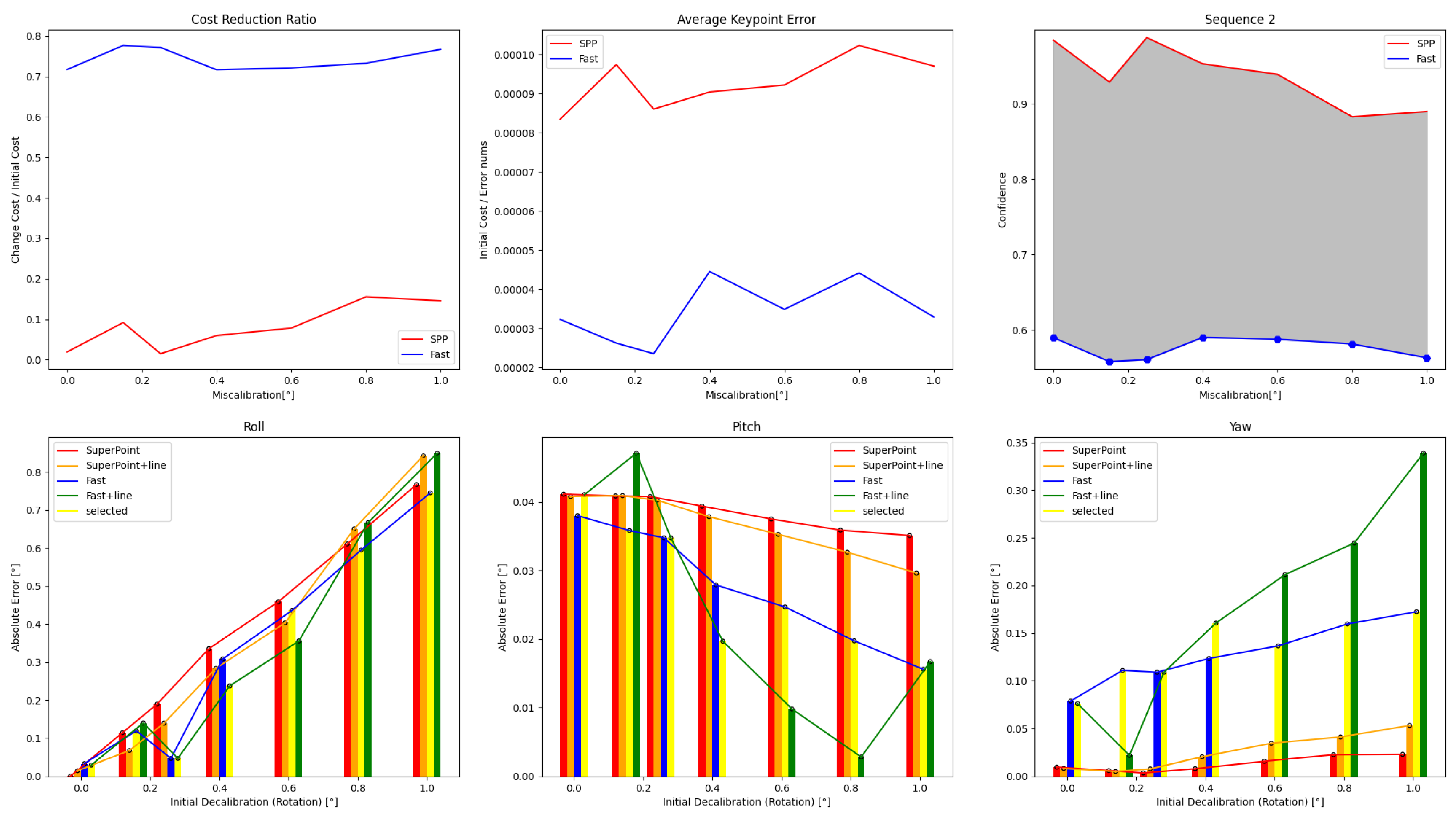
Figure 10.
During the pre-optimization process for Sequence 2, the confidence curves of two feature methods were analyzed and showed a clear distinction between them, indicating a significant difference in their effects. Our adaptive selection method opted for the direct method combined with line features for optimization under small initial perturbations.
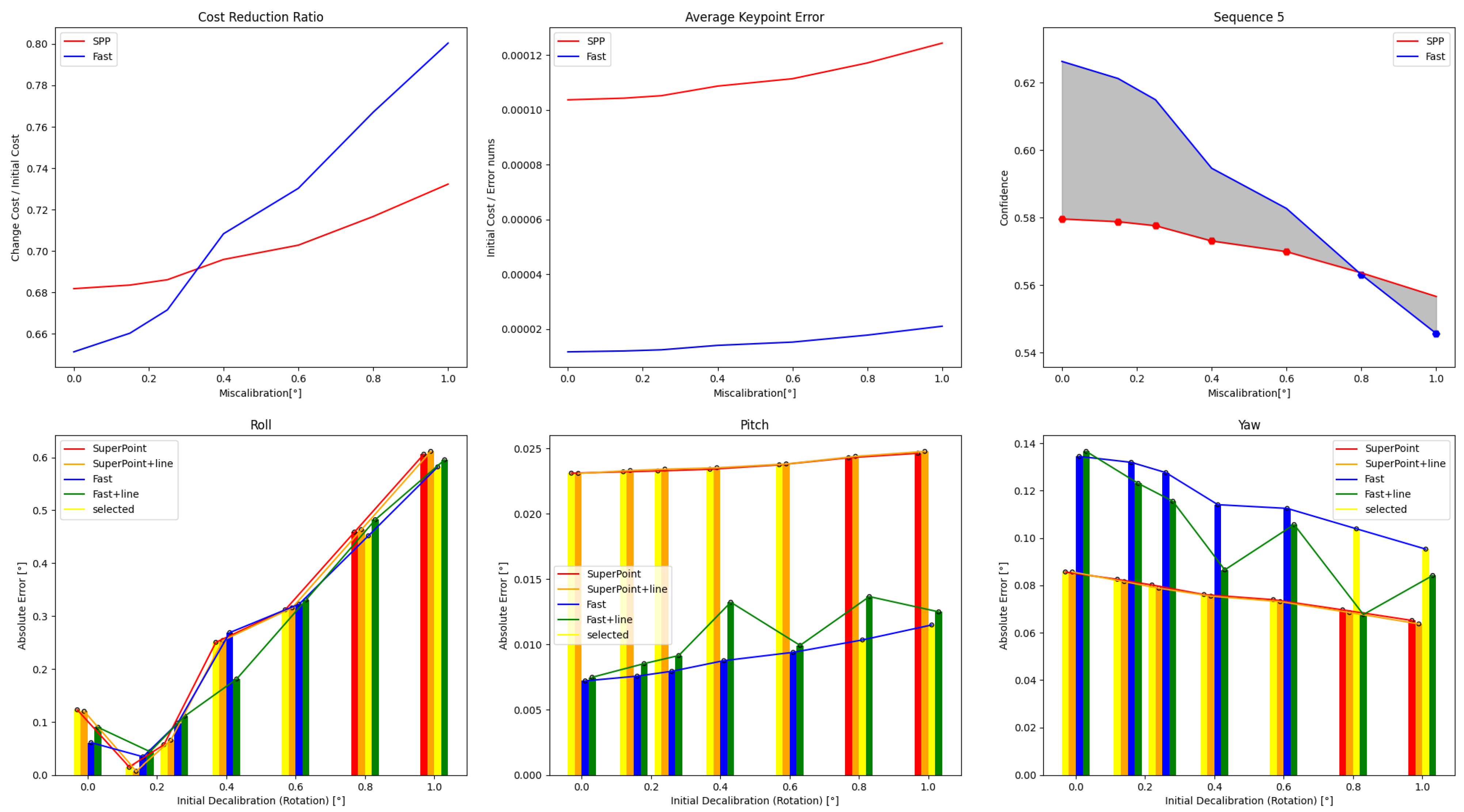
Figure 11.
For Sequence 5, different schemes can be selected under different initial values as the confidence reading curve has crossed.
Figure 11.
For Sequence 5, different schemes can be selected under different initial values as the confidence reading curve has crossed.
Figure 12.
The line features in Sequence 4 are of poor quality and have a high variance in length, which exceeds the threshold. Due to this, the adaptive strategy did not select these line features for optimization. Instead, a better solution was chosen to correct the roll.
Figure 12.
The line features in Sequence 4 are of poor quality and have a high variance in length, which exceeds the threshold. Due to this, the adaptive strategy did not select these line features for optimization. Instead, a better solution was chosen to correct the roll.
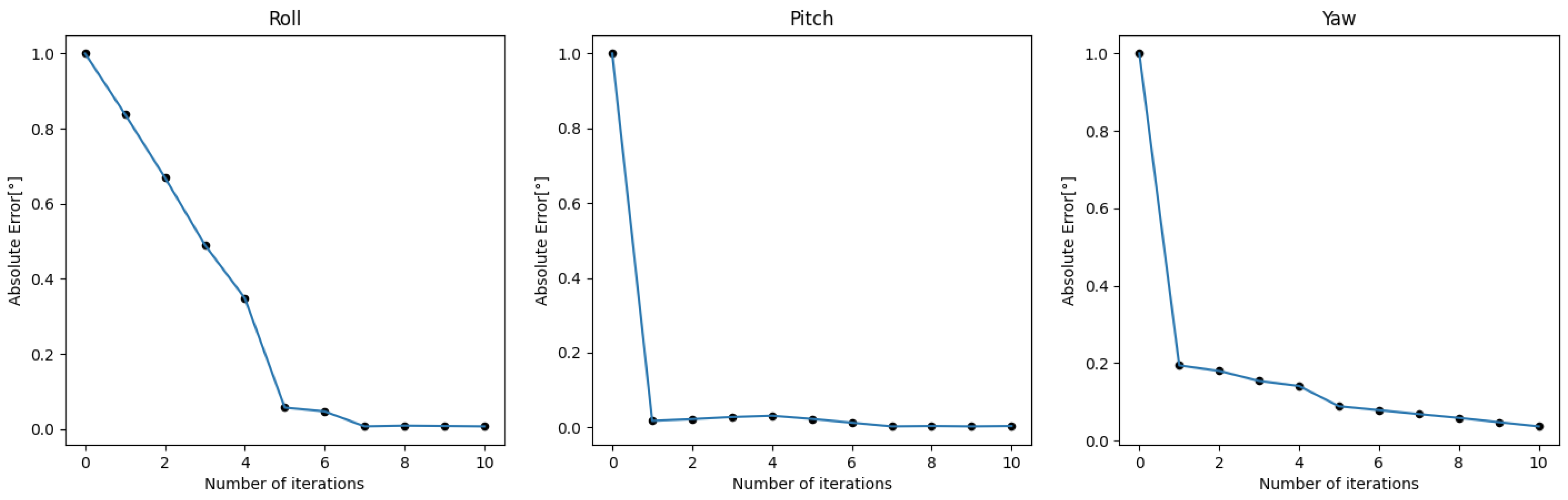
Figure 13.
The calibration effect of iterative optimization on Sequence 2.
Figure 13.
The calibration effect of iterative optimization on Sequence 2.
Figure 14.
Example of calibration results. In (a,c), the initial calibration values have an error of 1.0° in the roll, pitch, and yaw directions. After applying our calibration method, (b,d) can achieve a level close to the true values. The projection accuracy of objects such as car edges, poles, and trees has been enhanced.
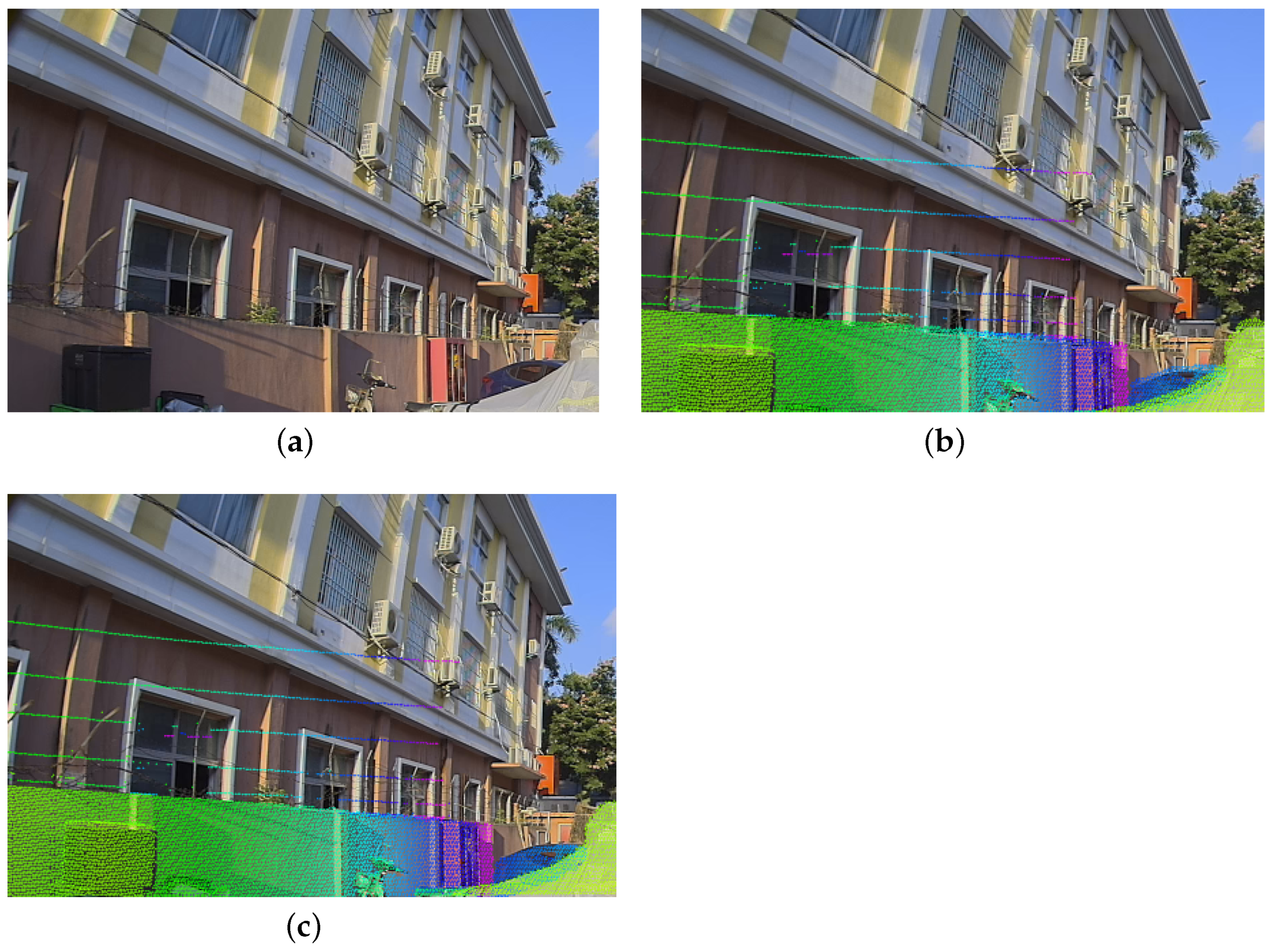
Figure 15.
Example of calibration results. To better visualize the results, we project the LiDAR point cloud onto the image plane, as shown in the figure above. (a) shows the original image. In (b), the device’s initial external parameters have a deviation of around 0.3° in the roll and 0.6° in the pitch. This results in noticeable projection deviations in walls and objects. In (c), after calibration through our iterative method, the error has been significantly reduced to less than 0.1°. Consequently, the projection is now essentially correct.
Table 1.
The time consumption of various calibration methods is as follows: (a) SPP represents SuperPoint feature point extraction and SuperGLUE feature matching method. (b) Fast represents the uniform sampling points extraction and optical flow matching method. (c) Line represents the AG3line extraction, optical flow matching, and fine-tuning method.
| Method | Detect [s] | Match [s] | Fine-Tuning [s] |
|---|
| SPP | 0.0115 | 0.0424 | - |
| Fast | | | - |
| Line | | | 0.0507 |


