A Cluster-Based Architecture to Structure the Topology of Parallel Wireless Sensor Networks


Abstract
:1. Introduction and Related Works
2. Problem Formulation and Application Environments
- -
- They could have a different transceiver to connect to other cluster nodes but the same transceiver to connect to the cluster head node.
- -
- They could use a different wireless protocol to connect to other cluster nodes but the same transceiver to connect to the cluster head node.
- -
- They could be using different types of technology to connect to other cluster nodes but the same transceiver to connect to the cluster head node.
- -
- They could be transmitting different types of data that is not understandable by other types of nodes, only by the same type of node and the cluster head node.
- -
- They could have different types of profiles.
- -
- They could be different types of devices.
- -
- When a new sensor joins the architecture, it will belong to the zone of its nearest central cluster sensor.
- -
- Due to processing consumption issues, the number of connections to the central cluster sensor should be limited, so when it reaches the maximum number of connections, the new sensor has to create a new cluster.
- -
- Sensors will have connections only with the same type of sensors of neighboring groups in a predefined distance or coverage area, but not with nodes from other groups that are not neighbors.
- -
- For energy saving purposes, when there are several sensors from other clusters in the sensor's coverage area, the one with higher capacity (which depends on the energy between other parameters that will be presented later) will be chosen as a neighbor.
- -
- The network formed by sensors of the same type will have its own routing protocol algorithm.
- -
- It could be used in any kind of system where an event or alarm is based on what is happening in a specific zone, but conditioned to the events that are happening in neighboring zones. One example is a group-based system to measure the environmental impact of a place (forest, marine reef, etc.). It could be better measured if the measurements are taken from the plants and from the trees in that place with different type of sensors. Each kind of measurement could be taken from different groups of sensors, but those groups of sensors have to be connected with the same type of sensors in order to estimate the whole environmental impact.
- -
- It could be used in body area sensor networks. The devices used to sense the body could be several types of sensor (pulse sensors, skin sensors, sweat sensors, etc.). A sensor may need to be connected with the same type of sensors of other zones of the body to form their specialized network in order to check the measurements of a specific parameter.
- -
- It could be used to build networks of sensors with the same profile that come from different communities (each community will be a cluster).
- -
- It could be used to build networks whose cluster can be formed by different types of devices such as mobiles, PDAs, PCs, sensors, but the requirement is for networks formed by the same type of devices.
- -
- It could be used for virtual wireless sensor network creation too.
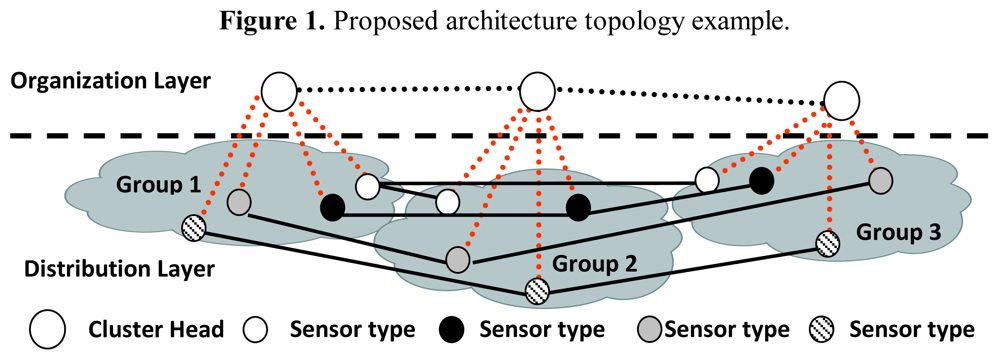
3. Architecture Proposal Description
3.1. Identifiers and Predefined Parameters
- -
- Max_con: Maximum number of supported connections from other nodes of the distribution layer.
- -
- Type: It identifies the type of node.
- -
- Max_distance: It is the maximum distance to be a neighbor. It is always shorter than or equal to the coverage area radius. It can be changed by the Received Signal Strength Indication (RSSI) value or by the Signal Noise Ratio (SNR) value. It is applied only to establish connections between CHs and their CMs and between CMs, but not between CHs because CH must have as many connections with other CHs as possible. We have proved in other works [31] that although inductive and hybrid methods provide higher reliable values, we are considering a hard environment where there might not be any previous training phase.
- -
- Position: It could be given manually or by GPS.
- -
- It will have other parameters that vary along its existence in the architecture:
- -
- Available_con: Number of available connections with other nodes of the distribution layer.
- -
- E: % of energy consumption.
- -
- L: % of available load. The load is the quantity of tasks the node is able to carry out at one time.
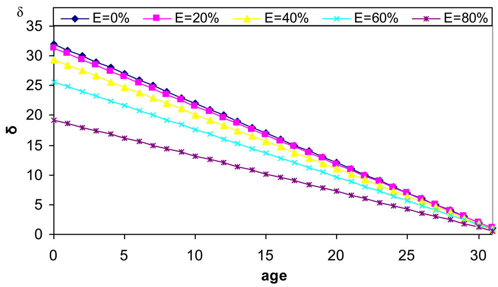
3.2. δ Parameter
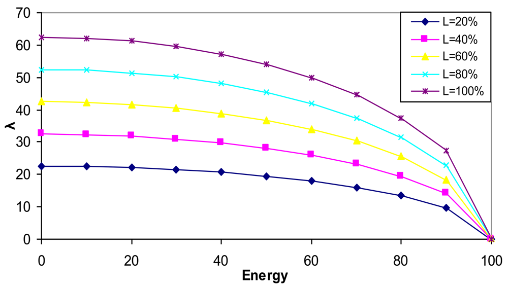
3.3. λ Parameter
4. Scalability
5. Architecture Proposal Operation and Fault Tolerance
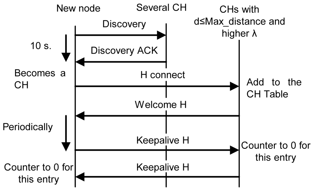
- If it does not receive any reply within 10 seconds, it becomes a CH, so it creates the cluster and waits for new nodes. Ten seconds have been chosen because it is enough time to receive a reply from a near node. Later replies will be from nodes which are either too far or too busy.
- If it receives some replies, but none of them are at a distance lower than the Max_distance, it becomes a CH and sends an “H connect” message to establish connections with selected CHs (based on their λ parameter). If the other CH confirms that connection, it adds this entry to its CH table and sends a “Welcome H” message with the last clusterID in the network. The CH will choose the next available clusterID for its cluster. Then, the new CH will send “Keepalive H” messages periodically with its clusterID to its neighbor CHs to indicate it is alive. If a CH does not receive a “Keepalive H” message from a CH for a dead time, it would erase that entry from the database. “Keepalive H” messages contain sender's clusterID and λ parameter. The CH also follows the new CM process described later. Messages sent in this case, when there is a new CH, are shown in Figure 9. Once the discovering process has finished CH node's network works as a regular OLSR network.
- If it receives one or several replies and all of them are within a distance lower than the Max_distance, it chooses the closest CH and in case of a draw, the one with highest λ parameter. Then, it sends an “M connect” message to establish a connection with the selected CH. If the other CH confirms that connection because it has not reached the maximum number of connections, it adds this entry to its CM table, sends a “Welcome M” message and the new node becomes a CM. If the CH does not agree the connection, the new node sends an “M connect” message to the second best CH and follows the same steps. This process is repeated until the new node reaches the last option. If the last option does not confirm the connection, the new node becomes a CH and follows the steps explained in case 2. When a CM receives a “Welcome M” message, it will know which its cluster is. It will send “Keepalive M” messages periodically to the CH to indicate it is alive. If the CH does not receive a “Keepalive M” message from a CM for a dead time, it will erase that entry from the database. “Keepalive M” messages contain the nodeID of the sender, its λ and its δ parameters. Steps followed when there is a new CM in this third case are shown in Figure 10.
Protocol Messages
6. Architecture Measurements
6.1. Test Bench
6.2. Network Measurements
6.3. Fault Tolerant Procedure
6.4. Bandwidth, Jitter, Delay, Lost Packets and Number of Packets with Errors
7. Protocol Comparisons
- -
- Topology updates overhead reduction.
- -
- The clustering structure is self-organized and adaptable.
- -
- Fully distributed operation.
- -
- New nodes do not have to be searched or initiated.
- -
- Broken routes cloud is repaired locally without rediscovery.
- -
- Reduction in the energy dissipation.
- -
- Broadcasts are done only by the boundary nodes.
- -
- The routing is source initiated.
- -
- Lower memory overhead.
- -
- Quite scalable.
7.1. Architecture Comparison
7.2. Measurement Comparisons
8. Conclusions
Acknowledgments
References
- Yick, J.; Mukherjee, B.; Dipak, D. Wireless Sensor Network Survey. Comput. Netw. 2008, 52, 2292–2330. [Google Scholar]
- Krco, S. Health Care Sensor Networks—Architecture and Protocols. Ad Hoc. Sensor Wireless Networks 2005, 1, 1–25. [Google Scholar]
- Mainwaring, A.; Szewczyk, R.; Anderson, J.; Polastre, J. Habitat Monitoring on Great Duck Island. Proceedings of ACM SenSys'04, Baltimore, MD, USA, November 2004.
- Summers, S.A. Wireless Sensor Networks for Firefighting and Fire Investigation; CS526 Project. UCCS: Colorado Springs, CO, USA, 2006. [Google Scholar]
- Yang, H.; Sikdar, B. A Protocol for Tracking Mobile Targets Using Sensor Networks. Proceedings of SNPA'03, Anchorage, AK, USA, May 2003; pp. 71–81.
- Jiang, M.; Li, J.; Tay, Y.C.; Cluster Based Routing Protocol (CBRP). August 1998. Available online: http://tools.ietf.org/html/draft-ietf-manet-cbrp-spec-01.txt (accessed on 3 December 2009).
- Ghosh, R.K.; Garg, V.; Meitei, M.; Raman, S.; Kumar, A.; Tewari, N. Dense Cluster Gateway Based Routing Protocol for Multi-Hop Mobile Ad Hoc Networks. Ad Hoc Netw. 2006, 4, 168–185. [Google Scholar]
- Yu, J.Y.; Chong, P.H.J. A Survey of Clustering Schemes for Mobile Ad Hoc Networks. IEEE Commun. Surv. Tutorials 2005, 7. [Google Scholar]
- Lin, C.R.; Gerla, M. Adaptive Clustering for Mobile Wireless Networks. IEEE J. Sel. Areas Commun. 1997, 15, 1265–1275. [Google Scholar]
- Ryu, J.H.; Song, S.; Cho, D.H. New Clustering Schemes for Energy Conservation in Two-Tiered Mobile Ad Hoc Networks. Proceedings of IEEE ICC'01, Helsinki, Finland, June 2001; pp. 862–866.
- Chatterjee, M.; Das, S.K.; Turgut, D. An On-Demand Weighted Clustering Algorithm (WCA) for Ad Hoc Networks. Proceedings of IEEE Globecom'00, San Francisco, CA, USA, November 27–December 1, 2000; pp. 1697–1701.
- Ohta, T.; Inoue, S.; Kakuda, Y. An Adaptive Multihop Clustering Scheme for Highly Mobile Ad Hoc Networks. Proceedings of 6th ISADS, Pisa, Italy, April 2003; pp. 293–300.
- Jin, Y.; Wang, L.; Kim, Y.; Yang, X. EEMC: An Energy-efficient Multi-level Clustering Algorithm For Large-scale Wireless Sensor Networks. Comput. Netw. 2008, 52, 542–562. [Google Scholar]
- Das, B.; Bharghavan, V. Routing in Ad Hoc Networks Using Minimum Connected Dominating Sets. Proceedings of IEEE ICC'97, Montreal, Canada, June 1997; pp. 376–380.
- Basu, P.; Khan, N.; Little, T.D.C. A Mobility Based Metric for Clustering in Mobile Ad Hoc Networks. Proceedings of IEEE ICDCSW' 01, Phoenix, AZ, USA, April 2001; pp. 413–418.
- Ren, Q.C.; Liang, Q.L. Energy-Efficient Medium Access Control Protocols for Wireless Sensor Networks. EURASIP J. Wirel. Commun. Netw. 2006, 2, 1–17. [Google Scholar]
- Amis, A.D.; Prakash, R. Load-Balancing Clusters in Wireless Ad Hoc Networks. Proceedings of 3rd IEEE ASSET, Richardson, TX, March 2000; pp. 25–32.
- Abbasi, A.A.; Younis, M. A Survey on Clustering Algorithms for Wireless Sensor Networks. Comput. Netw. 2007, 30, 2826–2841. [Google Scholar]
- Du, X.; Lin, F. Maintaining Differentiated Coverage in Heterogeneous Sensor Networks. EURASIP J. Wirel. Commun. Netw. 2005, 4, 565–572. [Google Scholar]
- Zou, Y.; Chakrabarty, K. Sensor Deployment and Target Localization in Distributed Sensor Networks. ACM Trans. Embed. Comput. Syst. 2004, 3, 61–91. [Google Scholar]
- Yuan, Y.; Chen, M.; Kwon, T. A Novel Cluster-Based Cooperative MIMO Scheme for Multi-Hop Wireless Sensor Networks. EURASIP J. Wirel. Commun. Netw. 2006, 2, 1–9. [Google Scholar]
- Ibriq, J.; Mahgoud, I. Cluster-Based Routing in Wireless Sensor Networks: Issues and Challenges. Proceedings of SPECTS'04, San Jose, CA, USA, July 2004; pp. 759–766.
- Lee, K.H.; Han, S.B.; Suh, H.S.; Lee, S.K.; Hwang, C.S. Authentication Based on Multilayer Clustering in Ad Hoc Networks. EURASIP J. Wirel. Commun. Netw. 2005, 5, 731–742. [Google Scholar]
- Kredo, K.; Mohapatra, P. Medium Access Control in Wireless Sensor Networks. Comput. Netw. 2007, 51, 961–994. [Google Scholar]
- Lloret, J.; Boronat, F.; Palau, C.; Esteve, M. Two Levels SPF-Based System to Interconnect Partially Decentralized P2P File Sharing Networks. Proceedings of ICAS-ICNS 2005, Papeete (Tahiti), French Polynesia, October 2005.
- Clausen, T.; Jacquet, P. Optimized Link State Routing Protocol (OLSR). RFC 3626. October 2003. Available online: http://www.ietf.org/rfc/rfc3626.txt (accessed on 3 December 2009).
- Perkins, C.; Belding-Royer, E.; Das, S. Ad Hoc On-Demand Distance Vector (AODV) Routing. RFC 3561. July 2003. Available online: http://www.ietf.org/rfc/rfc3561.txt (accessed on 3 December 2009).
- Johnson, D.; Hu, Y.; Maltz, D. The Dynamic Source Routing Protocol (DSR) for Mobile Ad hoc Networks for IPv4. RFC 4728. February 2007. Available online: http://www.ietf.org/rfc/rfc4728.txt (accessed on 3 December 2009).
- Park, V.; Corson, S. Temporally-Ordered Routing Algorithm (TORA) Version 1, Functional Specification, Internet Draft. June 2001. Available online: http://tools.ietf.org/id/draft-ietf-manet-tora-spec-04.txt (accessed on 3 December 2009).
- Chang, Y.C.; Lin, Z.S.; Chen, J.L. Cluster Based Self-Organization Management Protocols for Wireless Sensor Networks. IEEE Trans. Consum. Electron. 2006, 52, 75–80. [Google Scholar]
- Lloret, J.; Tomas, J.; Garcia, M.; Canovas, A. A Hybrid Stochastic Approach for Self-Location of Wireless Sensors in Indoor Environments. Sensors 2009, 9, 3695–3712. [Google Scholar]
- Heinzelman, W.R.; Chandrakasan, A.; Balakrishnan, H. Energy-efficient communication Protocol for Wireless Microsensor Networks. Proceedings of the 33rd Annual Hawaii International Conference on System Sciences, Maui, HI, USA, January 2000; 2.
- Bri, D.; Coll, H.; Garcia, M.; Lloret, J. A Multisensor Proposal for Wireless Sensor Networks. Proceedings of SENSORCOMM 2008, Cap Esterel, Côte d'Azur, France, August 2008.
- Wireshark Network Protocol Analyzer website. Available online: http://www.wireshark.org (accessed on 3 December 2009).
- Krishna, P.; Vaidya, N.H.; Chatterjee, M.; Pradhan, D.K. A Cluster-Based Approach for Routing in Dynamic Networks. ACM SIGCOMM Comput. Commun. Rev. 1997, 27, 49–64. [Google Scholar]
- Bechler, M.; Hof, H.; Kraft, D.; Pählke, F.; Wolf, L. A Cluster-Based Security Architecture for Ad Hoc Networks. proceedings of INFOCOM 04, Hong Kong, China, March 2004; pp. 2393–2403.
- Leng, S.; Zhang, L.; Fu, H.; Yang, J. A Novel Location-Service Protocol Based on k-Hop Clustering for Mobile Ad Hoc Networks. IEEE Trans. Veh. Technol. 2007, 56, 810–817. [Google Scholar]
- Muruganathan, S.D.; Ma, D.C.F.; Bhasin, R.I.; Fapojuwo, A.O. A Centralized Energy-Efficient Routing Protocol for Wireless Sensor Networks. IEEE Commun. Mag. 2005, 43, 8–13. [Google Scholar]
- Shih, T.F.; Yen, H.C. Core Location-Aided Cluster-Based Routing Protocol for Mobile Ad Hoc Networks. proceedings of WSEAS ICC 06, Vouliagmeni, Athens, Greece, July 2006; pp. 223–228.
- Wang, Y.; Chen, H.; Yang, X.; Zhang, D. Cluster Based Location-Aware Routing Protocol for Large Scale Heterogeneous MANET. Proceedings of IMSCCS 2007, Iowa City, IA, USA, August 2007; pp. 366–373.
- Chatterjee, M.; Das, S.K.; Turgut, D. WCA: A Weighted Clustering Algorithm for Mobile Ad Hoc Networks. Cluster Comput. 2002, 5, 193–204. [Google Scholar]
- Shen, C.; Srisathapornphat, C.; Liu, R.; Huang, Z.; Jaikaeo, C.; Lloyd, E. CLTC: A Cluster-based Topology Control Framework for Ad Hoc Networks. IEEE Trans. Mob. Comput. 2004, 3, 18–32. [Google Scholar]
- Wen, C.Y.; Sethares, W.A. Automatic Decentralized Clustering for Wireless Sensor Networks. EURASIP J. Wirel. Commun. Netw. 2005, 5, 686–697. [Google Scholar]
- Chen, J.; Yu, F. A Uniformly Distributed Adaptive Clustering Hierarchy Routing Protocol. Proceedings of the ICIT 2007, Shenzhen, China, March 2007.
- Younis, O.; Fahmy, S. Distributed Clustering in Ad Hoc Sensor Networks: A Hybrid, Energy-Efficient Approach. Proceedings of INFOCOM 2004, Hong Kong, China, March 2004.
- Hollerung, T.D. The Cluster-Based Routing Protocol; Winter semester 2003/2004University of Paderborn: Paderborn, Germany, 2004. [Google Scholar]


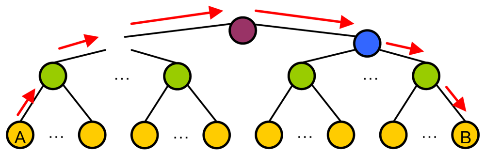
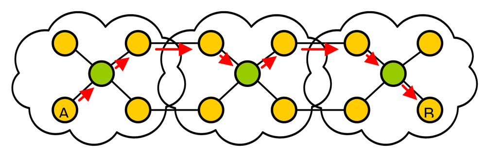
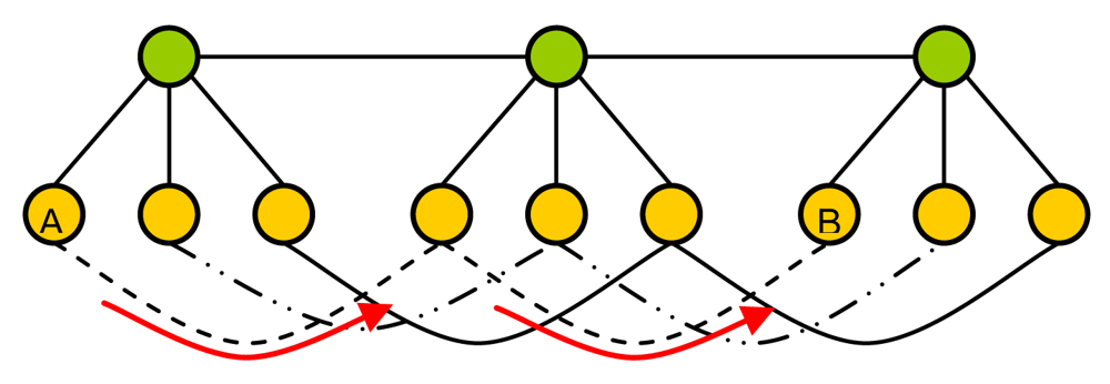
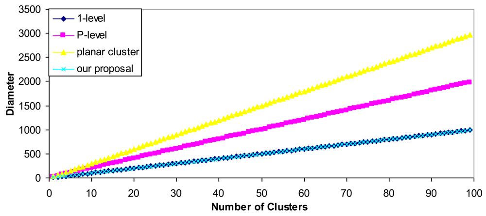
| Type of cluster | Diameter (d) |
|---|---|
| 1-level cluster | K + 1 |
| P-level cluster | 2·p |
| Planar cluster with one hop | 3·k – 1 |
| Our proposal | K – 1 |
| Node number | Type of node | X | Y |
|---|---|---|---|
| 1 | a | 0 | 0 |
| 2 | b | 50 | 0 |
| 3 | a | 100 | 150 |
| 4 | b | 50 | 100 |
| 5 | c | 25 | 50 |
| 6 | c | 100 | 75 |
| 7 | a | 200 | 25 |
| 8 | b | 150 | 100 |
| 9 | a | 200 | 175 |
| 10 | c | 150 | 50 |
| 11 | d | 125 | 125 |
| 12 | b | 175 | 175 |
| 13 | c | 200 | 75 |
| 14 | d | 125 | 25 |
| 15 | d | 50 | 25 |
| Table 2b. Neighbor connections. | |||
|---|---|---|---|
| Node number | Role | Connections with CH | Connections with CM |
| 1 | CH | 3, 7, 9 | 2, 5, 15 |
| 2 | CM | 1 | 4 |
| 3 | CH | 1, 7, 9 | 4, 6, 11 |
| 4 | CM | 3 | 2, 8 |
| 5 | CM | 1 | 6 |
| 6 | CM | 3 | 5, 10 |
| 7 | CH | 1, 3, 9 | 8, 10, 14 |
| 8 | CM | 7 | 4, 12 |
| 9 | CH | 1, 3, 7 | 12, 13, 16 |
| 10 | CM | 7 | 6, 13 |
| 11 | CM | 3 | 14, 16 |
| 12 | CM | 9 | 8 |
| 13 | CM | 9 | 10 |
| 14 | CM | 7 | 11, 15 |
| 15 | CM | 1 | 14 |
| 16 | CM | 9 | 11 |
| Architecture | Overlapping nodes | Uses other routing protocols | Number of messages | New node cluster's selection | Purpose | Node Fault Tolerance | Cluster Head selection |
|---|---|---|---|---|---|---|---|
| P. Krishna et al. [35] | Yes | Just one at a time | 16 | Proximity | Routing | No | n/a |
| CBRP [6] | Yes | No | 6 | nodeID | Routing | No | Lowest node ID |
| Marc Bechler et al. [36] | No | Just one at a time | n/p | n/p | Security | Yes, but very weak | Trusted node, but not explained what happens if there are several trusted nodes. |
| KCLS [37] | No | No | 13 + GPS protocol | Distance to the head node less than k hops | Location Service | Yes | Mobility threshold |
| Chunhung R. Lin [9] | No | Just one at a time | n/p | nodeID | Bandwidth allocation | Yes | Lowest node ID |
| LEACH [34] | No | No | n/p | received signal strength | Energy optimization | No | Random rotation |
| BCDCP [38] | No | No | n/p | Location | Energy optimization | No | Random |
| CLACR [39] | No | No | 11 | Location | Routing | Just for location servers | Closest to the cluster center position |
| CBLARHM [40] | No | No | 17+ GPS | Relative distance, velocity and time | Routing | No | Node-Weight heuristic |
| WCA [41] | No | Just one at a time | n/p | Degree difference and proximity | General purpose | No | Combined weight metric |
| CLTC [42] | No | Just one at a time | 10+ GPS | Coverage area | Topology control | No | n/p |
| Our proposal | No | Yes and it could use many simultaneously. | 14 | Proximity + capacity parameter | Create parallel networks | Yes | Promotion Parameter |
| Reference | Type of measurements | Purpose |
|---|---|---|
| [34] | It gives the simulations of the average cluster size and the number of clusters versus the degree of the nodes. | Parameters related with the cluster size and the number of clusters |
| [40] | It gives the average number of cluster heads versus the number of nodes and the cluster size versus the number of nodes. | |
| [42] | It gives the average number of clusters versus the transmission range or the maximum displacements | |
| [13] | It provides the energy consumption versus the distance to the nodes and the number of nodes, the number of alive nodes versus the round and the energy consumed versus the number of rounds. | Energy issues |
| [19] | It shows the energy consumption versus the number of L-sensors, average number of working nodes versus the number of sensors and the energy consumption versus the average desired coverage degree. | |
| [32] | It gives the number of nodes alive versus the time, the energy dissipation versus the percentage of nodes that are cluster heads, and the energy dissipation versus the network diameter. | |
| [37] | It compares several cluster-based protocols versus the number of rounds, number of messages received versus the energy dissipation and energy consumed and the number of nodes alive as a function of network area. | |
| [43] | It shows the measurements of the number of alive nodes versus the time, the energy dissipation versus the time and the energy dissipation in the setup phase. | |
| [44] | It shows the percentage of energy consumed versus the cluster radius, the average cluster head residual energy versus the cluster radius and the cluster energy dissipated versus the number of nodes. |
© 2009 by the authors; licensee Molecular Diversity Preservation International, Basel, Switzerland. This article is an open access article distributed under the terms and conditions of the Creative Commons Attribution license (http://creativecommons.org/licenses/by/3.0/).
Share and Cite
Lloret, J.; Garcia, M.; Bri, D.; Diaz, J.R. A Cluster-Based Architecture to Structure the Topology of Parallel Wireless Sensor Networks. Sensors 2009, 9, 10513-10544. https://0-doi-org.brum.beds.ac.uk/10.3390/s91210513
Lloret J, Garcia M, Bri D, Diaz JR. A Cluster-Based Architecture to Structure the Topology of Parallel Wireless Sensor Networks. Sensors. 2009; 9(12):10513-10544. https://0-doi-org.brum.beds.ac.uk/10.3390/s91210513
Chicago/Turabian StyleLloret, Jaime, Miguel Garcia, Diana Bri, and Juan R. Diaz. 2009. "A Cluster-Based Architecture to Structure the Topology of Parallel Wireless Sensor Networks" Sensors 9, no. 12: 10513-10544. https://0-doi-org.brum.beds.ac.uk/10.3390/s91210513