Scrub Typhus Incidence Modeling with Meteorological Factors in South Korea

Abstract

Since its recurrence in 1986, scrub typhus has been occurring annually and it is considered as one of the most prevalent diseases in Korea. Scrub typhus is a 3rd grade nationally notifiable disease that has greatly increased in Korea since 2000. The objective of this study is to construct a disease incidence model for prediction and quantification of the incidences of scrub typhus. Using data from 2001 to 2010, the incidence Artificial Neural Network (ANN) model, which considers the time-lag between scrub typhus and minimum temperature, precipitation and average wind speed based on the Granger causality and spectral analysis, is constructed and tested for 2011 to 2012. Results show reliable simulation of scrub typhus incidences with selected predictors, and indicate that the seasonality in meteorological data should be considered.

1. Introduction

Scrub typhus is a rickettsial disease caused by intracellular bacteria Orientia tsutsugamushi and is transmitted by infection to humans through various species of infected Trombiculidae mites that feed on lymph and tissue fluid [1]. It is widely known as an endemic disease in Japan and is widely distributed within a 13 million km² area of Southeast Asia and the Pacific Rim regions and approximately 1 billion persons are estimated at risk of the disease [2]. In South Korea (hereinafter referred to as Korea), it was first reported in 1951 and it reappeared in 1986 [3]. Since then scrub typhus incidences have been reported every year. Now it is considered as one of the most prevalent diseases in the southwestern provinces of Korea [4]. Generally, vector-borne diseases are transmitted by arthropods which can be greatly affected by climate [5]. Considering the results of Choi [6], who suggested that meteorological characteristics in Korea appear to have actually changed from 2000 onwards, it can therefore be inferred that scrub typhus is also affected by climate change.

Kalra and Rao [7] claimed that scrub typhus occurred in Kashmir, India, in a relatively temperate climate. There are many studies that have contributed to the knowledge on how scrub typhus is related to meteorological factors and is forecasted. The seasonal occurrence of scrub typhus varies according to climate in different countries [1], and the disease is found to occur more commonly during rainy season [8,9]. Kasuya [10] investigated the relationship between scrub typhus and meteorological factors using regression analysis. Kawamura et al. [11] analyzed the relationship between scrub typhus and climate type which reflects the behavior and population of Trombiculidae. Also, Zhang et al. [12] analyzed the relationship of scrub typhus and meteorological factors by regression analysis in Shijiazhuang City, China. The seasonality of scrub typhus suggests that meteorological variables might influence the spread of the disease [13].

Since climate change is now accepted as real, this change affects infectious disease pathogens and agents that influence the duration of infection, disease distribution [14,15] and spread to various vector and rodent-borne diseases [16,17,18,19,20]. Hence, recent studies have focused on determining the correlation between scrub typhus and meteorological factors and their influence on the disease [1,21,22,23,24,25,26,27]. Li et al. [28] found annual mean, maximum and minimum temperature and precipitation values to be correlated with scrub typhus, and Li et al. [13] showed that scrub typhus and monthly temperature, duration of sunshine, and rainfall were positively associated. Kim and Jang [25] also showed that temperature and humidity were closely correlated with scrub typhus in Korea. Kuo et al. [29] have reported a higher risk for scrub typhus infection in the endemic area with a higher normalized difference vegetation index (NDVI) [30] in Taiwan. Especially, Yang et al. [31] showed that the temperature with time-lag is important for the scrub typhus occurrence. However, very few studies have been completed on simulating or predicting the incidences with meteorological factors.

The objective of this study, therefore, is to investigate the incidence of scrub typhus and its correlation with meteorological factors and to construct a model, which employs Artificial Neural Network (hereinafter referred to as ANN), for incidences in Korea. By simulating the scrub typhus incidences in Korea, based on observed meteorological factors, the model can provide basic data of disease control for public health agencies. For this study, data on monthly scrub typhus occurrences and meteorological factors from 2001 to 2012 were collected. The constructed model was tested for 2011 and 2012 and the trend of incidences and seasonality were analyzed.

2. Scrub Typhus in Korea

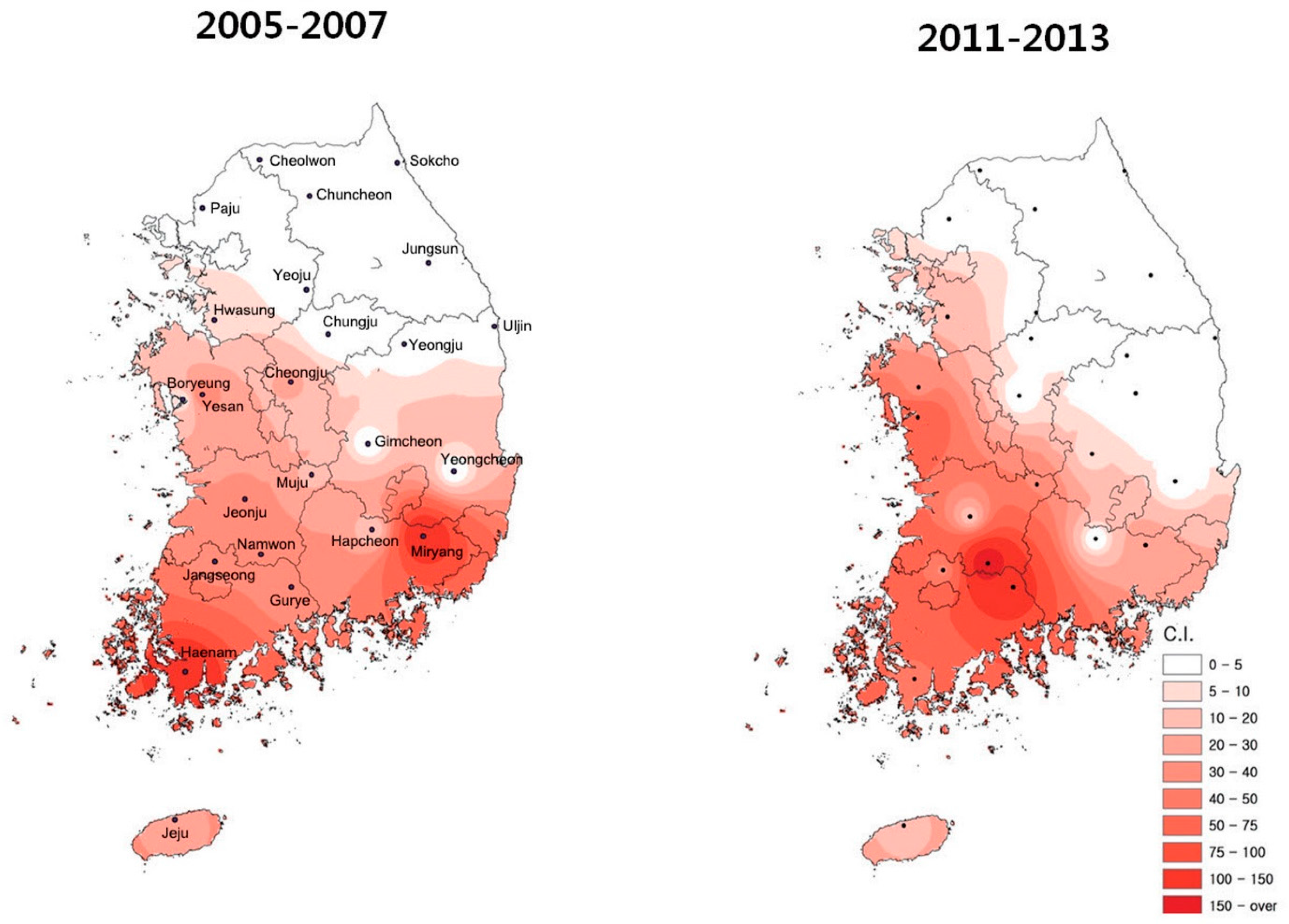
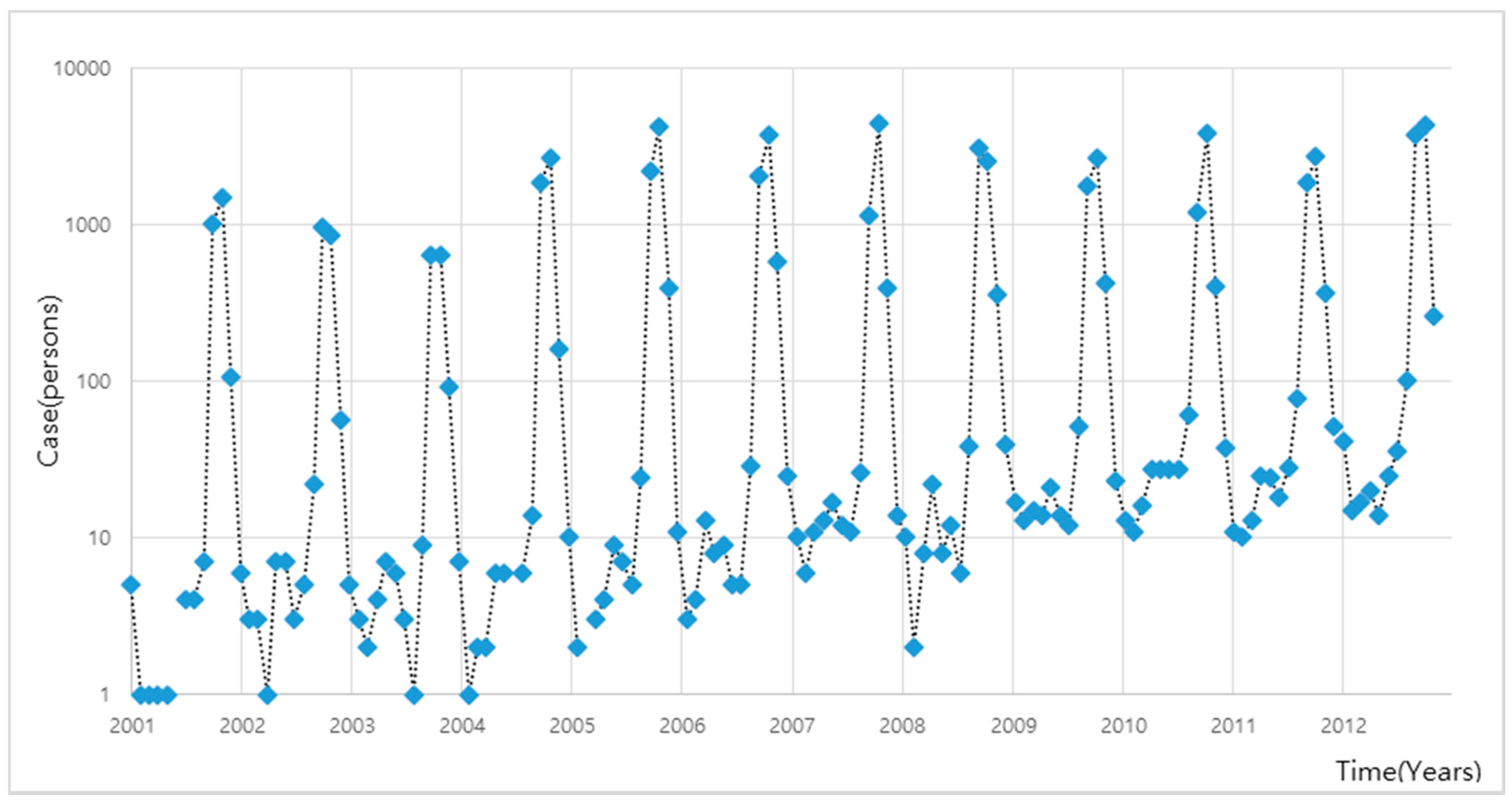
2.1. Incidence Trend of Scrub Typhus

Since the reappearance of scrub typhus in 1986, cases of incidences have remarkably increased [32]. Especially, the occurrence of scrub typhus has significantly increased from 2000 onwards and it is continuously increasing. For example, 238 patients were reported in 1994, 4698 cases in 2004, and 10,365 cases in 2013, showing a 24% increase annually after 2000 onwards and it is now considered as one of the most prevalent diseases affecting humans in southwestern provinces of Korea [4]. Infection through Leptotrombidium (hereinafter referred to as L. scutellare and L. pallidum) is the reported cause of the scrub typhus in Korea, and L. akamushi hasn’t been reported yet [33], L. scutellare is the major cause of scrub typhus in Korea [34].

Scrub typhus is transmitted to humans through larvae bites of trombiculid mites and its habitat is located in low trees and bushes [35]. The mites that carry scrub typhus are affected by climatic conditions during the life-cycle [11]. Therefore, in Korea, an increase of scrub typhus infection is strongly related to the change in meteorological conditions [36,37] caused by climate change [38].

2.2. Data Collection

For this study, monthly data of the designated infectious diseases between 2001 and 2012, from the Center for Disease Control & Prevention [33], were utilized for obtaining data on the scrub typhus incidences of whole Korea. Data from 2001 to 2010 were used for calibration and data from 2011 to 2012 were used for validation. Also, meteorological data were obtained from the Korea Meteorological Administration (KMA). But the geographical distribution of Trombiculidae, which is mainly responsible for scrub typhus, is concentrated in the southwestern province of Korea [39].

We collected 24 meteorological observatory (2001 to 2007) and 25 meteorological observatory (2008 to 2013) meteorological data, and these data were weighted averaged into one, which considered the spatial distributions (C.I. number of L. scutellare in Figure 1) of L. scutellare as in study by [39]. Meteorological data included in the analysis were monthly average, maximum and minimum air temperatures (°C), precipitation (mm), relative humidity (%), wind speed (m/s), duration of sunshine (hours), and cloud amount, which are known as responsible factors for scrub typhus [31,40,41,42]. Also, some studies have indicated that land use affects scrub typhus [29], but Jin et al. [43] showed the land use changes did not affect Scrub typhus. Hence, it was not taken into account in this study. The collected meteorological data are shown in Figure 2 and scrub typhus in Figure 3.

Figure 1. Geographical distribution of Orientia tsutsugamushi vector, L. scutellare density in Korea [39]; C. I. (confidence interval) color and number indicated the collected cases of chiggers that has scrub typhus (L. scutellare).

Figure 1. Geographical distribution of Orientia tsutsugamushi vector, L. scutellare density in Korea [39]; C. I. (confidence interval) color and number indicated the collected cases of chiggers that has scrub typhus (L. scutellare).

Figure 2. Weighted average meteorological data from Korea [44].

Figure 2. Weighted average meteorological data from Korea [44].

Figure 3. Scrub typhus incidence cases in Korea [33].

Figure 3. Scrub typhus incidence cases in Korea [33].

3. Methodology

Many studies consider meteorological factors, which are related to epidemic diseases, as a statistical variable, not a time series, but Yang et al. [31] suggested scrub typhus displayed a time-lag effect, and Kim and Jang [25] showed that scrub typhus had a correlation with meteorological factors in the summer season in Korea. Therefore, this study considered meteorological and scrub typhus data as time series. When doing so, we employed the Granger causality and cross-spectral analysis to determine meteorological factors that have correlation with scrub typhus and time-lag, and then constructed a scrub typhus incidence model with an artificial neural network.

3.1. Granger Causality

Granger [45] suggested the idea of causality as a tool to determine that variable (or time series) whereby X causes variable Y if knowing X helps predict the future of Y. This is referred to as the Granger causality whereby X can be identified as the cause of Y when the inclusion of past observations of X reduces the prediction error of Y in a linear regression model, as compared to a model which includes only previous values of Y. Therefore, the Granger causality has been widely employed in many fields that need to determine the cause one among the set of unclear variables [46]. The Granger causality can be described by a bivariate autoregressive model as:

$$\text{X}\left(\text{t}\right)= {\displaystyle \sum }_{i=1}^k{A}_{1}X\left(t-i\right)+ {\displaystyle \sum }_{i=1}^k{A}_{2}Y\left(t-i\right)+ {ϵ}_1\left(t\right)$$

$$\text{Y}\left(\text{t}\right)= {\displaystyle \sum }_{i=1}^k{B}_{1}Y\left(t-i\right)+ {\displaystyle \sum }_{i=1}^k{B}_{2}X\left(t-i\right)+ {ϵ}_2\left(t\right)$$

(1)

where X and Y are each time series, $t$ denotes the index of time step in the time series, $k$ is the maximum number of lag in each time series, A and B are the model parameters of each time series, and ϵ₁ and ϵ₂ are the error measurements of model. If the variance of ϵ₁ or ϵ₂ is reduced by the inclusion of Y or X, it is evident that X is the cause of Y or Y is the cause of X. In this case, A or B is significantly different from zero and it can be estimated by the logarithm of the corresponding F-statistic [47].

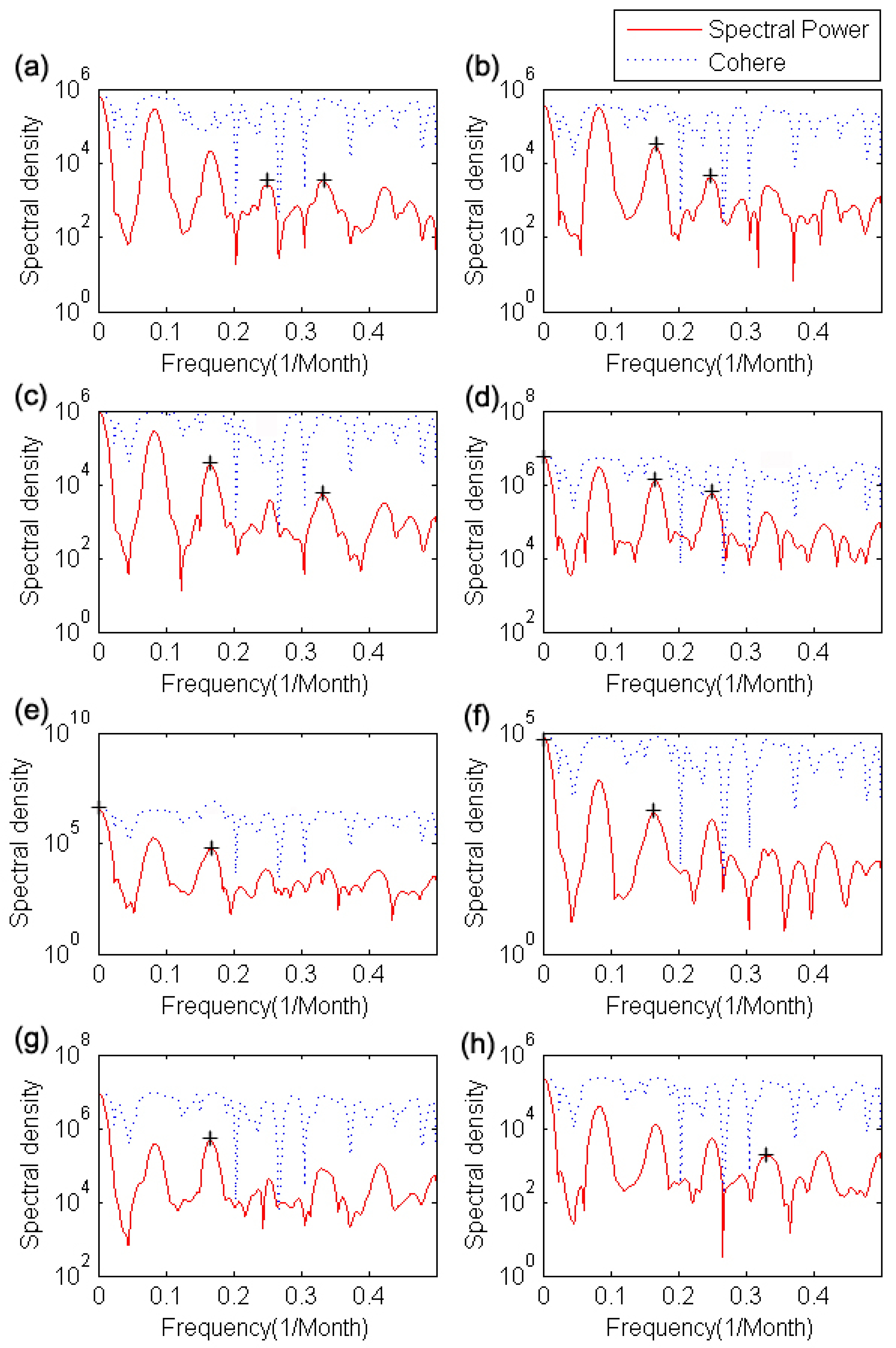
3.2. Cross Spectrum and Wavelet Spectrum

Autospectrum or cross spectrum is a method to explain the distribution of correlation (or cross-correlation) or variance of frequency drawn from a single or multiple data [48]. It is useful to investigate the changing frequency of meteorological data [49]. Autocorrelation function can be obtained by dividing the autocovariance by σ², the variance of $\text{X}\left(\text{t}\right)$. Autospectral function ${\text{X}}_{\text{X}}\left(\text{n}\right)$ can be obtained by applying the Fourier transform to the autocorrelation function ($n$ is the frequency of data), so autospectral analysis gives periodic information of each time series. Like the autospectrum, cross spectral analysis can also be applied to cross-covariance of two time series $\text{X}\left(\text{t}\right),\text{ Y}\left(\text{t}\right)$ and can be also used to differentiate the relevant covariance of two time series data set to have lag $\text{k}$. Cross spectral function ${\text{X}}_{\text{xy}}(n$) of two times series can be determined using Equations (2) and (3):

$${\text{VAR}}_{\text{X}}\left(\text{k}\right)=\frac{1}{\text{N}-\text{k}-1}{\displaystyle \sum }_{\text{t}=1}^{\text{N}-\text{k}}\left({\text{X}}_{\text{t}}-\stackrel{\text{X}}{¯}\right)\left({\text{X}}_{\text{t}+\text{k}}-\stackrel{\text{X}}{¯}\right)$$

(2)

$${\text{X}}_{\text{XY}}\left(n\right)={\displaystyle \sum }_{\text{k}=0}^{\text{N}}\left[\frac{{\text{COV}}_{\text{XY}}\left(\text{k}\right)}{{\text{σ}}_{\text{X}}{\text{σ}}_{\text{Y}}}\right]{\text{e}}^{\frac{\text{i }2\text{π f k}}{n}}$$

(3)

where N is the number of data and t and ∆t are the time step and time interval in the each time series, and k denotes the time lag. So, cross-spectrum gives correlation as a frequency function and it can be used to determine the phase difference between two time series. Also, using the cross- spectrum on two time series, coherency can be calculated and information about the frequency between the two (see Equation (4)) can be obtained. Coherency between two time series is defined as:

$${\text{C}}_{\text{xy}}\left(\text{n}\right)=\frac{{\left|{\text{X}}_{\text{xy}}\left(n\right)\right|}^2}{{\text{X}}_{\text{x}}\left(n\right){\text{ X}}_{\text{y}}\left(n\right)}$$

(4)

where ${\text{C}}_{\text{xy}}$ is the magnitude-squared coherence, and ${\text{X}}_{\text{x}}{\text{ and X}}_{\text{y}}$ are the autospectral densities of the two time series. The coherence value will always satisfy $0<C_{\text{xy}}<1$ and it can be used to estimate the causality between the input and output when the data are ergodic and the system function is linear [50].

Also, wavelet spectrum (transformation) is the method to expand time series into time frequency space and it can be used to find localized intermittent periodicities [51]. Especially, continuous wavelet transform (CWT) is desirable to examine two time series that may be expected to be linked in some way [52]. The CWT of the time series is defined as:

$$W_X\left(\text{s},\text{t}\right)=\text{ X}\left(\text{t}\right)\times {\phi }_s\left(\text{t}\right)$$

(5)

$${\phi }_s\left(\text{t}\right)= {\pi }^{-1/4} \times e^{i\omega t}\times e^{\frac{t^2}{2}}$$

(6)

where ${\phi }_s\left(\text{t}\right)$ is the Morlet wavelet [53] with scale $\text{s}$ and the power of wavelet can be defined as ${\left|{W_n}^X\left(\text{s}\right)\right|}^2$. Cross wavelet transform with two time series $\text{X}\left(\text{t}\right),\text{ Y}\left(\text{t}\right)$ can be defined as $W_{XY}\left(s,t\right)= W_X\left(\text{s},\text{t}\right){W_Y}^{*}\left(s,t\right)$ and asterisk denotes complex conjugation, so we further define the cross wavelet power as $\left|W_{XY}\right|$. This complex argument arg ($W_{XY}$) can be interpreted as the local relative phase between two time series $\text{X}\left(\text{t}\right),\text{ Y}\left(\text{t}\right)$ in the time frequency space [52].

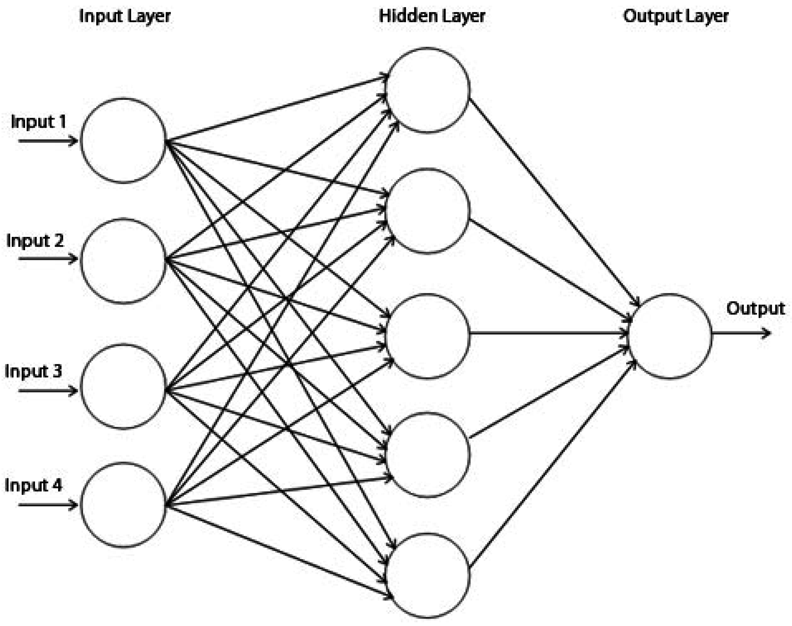
3.3. Artificial Neural Network

Kihoro et al. [54] have shown that ANNs are better than Autoregressive Integrated Moving Average (ARIMA) models in their forecasting ability for seasonal time series, so we employed an ANN for scrub typhus forecasting. The ANN [55] mimics the structure and functions of a biological neural system in which neurons are connected through nodes [56]. Since the perceptron was proposed to categorize information patterns [57], ANNs have been widely used to recognize nonlinear relationships between different variables. The ANN is composed of three layers: the input layer represents observed meteorological data, the output layer produces simulated incidence cases as a result of network and the hidden layer is constituted of a network of neurons (non-linear functions) that are trained to recognize patterns of observations.

Figure 4. ANN schematization [58]. Input i is the input set, output is the result of network delay and each circle represents neural network.

Figure 4. ANN schematization [58]. Input i is the input set, output is the result of network delay and each circle represents neural network.

The back-propagation algorithm has been used to train the network [59]. The Levenberg-Marquardt-QNBP algorithm has been used to optimize the parameters of the network and it is known to produce good results for non-linear problems, such as related meteorological data [59,60,61].

4. Scrub Typhus Modeling with Meteorological Factors

4.1. Predictor Selection and Construction of Incidence Model

Many previous studies [25,62,63] show that scrub typhus and meteorological data in Korea have seasonality. Strictly, it may be due to error in analysis [64], as Briët et al. [65] showed that in most cases strong correlation between malaria and precipitation that is considered most highly correlated with many epidemic diseases in Sri Lanka was spurious. Therefore, monthly mean value of 20 years was subtracted from the values of each meteorological factor used in this study. This method is widely used to remove seasonality [66,67]. Figure 5 shows the correlation matrix between scrub typhus and each meteorological data set which was detrended.

Figure 5. Scatter plot of scrub typhus and each variable, the number indicates Pearson’s correlation coefficient : S.T; Scrub typhus, T(1); mean temperature (°C), T(2); minimum temperature (°C), T(3); maximum temperature (°C), Pr.; precipitation (mm), H; relative humidity (%), W.S.; mean wind speed (m/s), Sun; duration of sunshine (hours), Cloud; cloud amount, and red marks indicate that the correlation coefficient has a statistically significant meaning, and the histogram is a non-dimensional plot.

Figure 5. Scatter plot of scrub typhus and each variable, the number indicates Pearson’s correlation coefficient : S.T; Scrub typhus, T(1); mean temperature (°C), T(2); minimum temperature (°C), T(3); maximum temperature (°C), Pr.; precipitation (mm), H; relative humidity (%), W.S.; mean wind speed (m/s), Sun; duration of sunshine (hours), Cloud; cloud amount, and red marks indicate that the correlation coefficient has a statistically significant meaning, and the histogram is a non-dimensional plot.

As a result of Figure 5, it seems that it is hard to find suitable meteorological factors to construct a model to estimate scrub typhus incidences. Kim and Jang [25] reported that scrub typhus is highly correlated with meteorological conditions in the summer season. Therefore, we employed the Granger causality and cross-spectral analysis to determine what the proper predictor and time-lag (k) between scrub typhus and meteorological factors are. As Song et al. [68] and Kim and Jang [25] show that scrub typhus in Korea mainly spawns in the summer season, the Granger causality was calculated for one to six month time lags and detrended meteorological factors, and results are shown in Table 1.

Table 1. Granger causality result with scrub typhus and detrended meteorological factors.

Meteorological Factor	Number of Lag (k)
	1	2	3	4	5	6
Mean Temp. (°C)	61.74 **	3.60	1.62	3.87	6.02 *	6.06 *
Min. Temp. (°C)	4.01	0.96	1.96	3.55	7.02 *	7.60 *
Max. Temp. (°C)	89.86 **	14.77 **	12.14 *	5.85	5.18	5.32
Precipitation (mm)	3.67	4.00	4.61	4.19	4.03	6.14 *
Relative Humidity (%)	1.37	3.73	5.38	7.81 *	9.35 *	8.26 *
Wind Speed (m/s)	1.68	1.97	2.11	29.11 **	40.10 **	43.06 **
Duration of sunshine (h)	3.61	3.23	5.43	3.90	3.10	5.10
Cloud amount	4.37	4.68	5.53	4.44	3.90	4.15

* and ** indicate statistically significance level at $\text{p}=0.1$ and $\text{p}=0.05$.

Table 1. Granger causality result with scrub typhus and detrended meteorological factors.

Meteorological Factor	Number of Lag (k)
	1	2	3	4	5	6
Mean Temp. (°C)	61.74 **	3.60	1.62	3.87	6.02 *	6.06 *
Min. Temp. (°C)	4.01	0.96	1.96	3.55	7.02 *	7.60 *
Max. Temp. (°C)	89.86 **	14.77 **	12.14 *	5.85	5.18	5.32
Precipitation (mm)	3.67	4.00	4.61	4.19	4.03	6.14 *
Relative Humidity (%)	1.37	3.73	5.38	7.81 *	9.35 *	8.26 *
Wind Speed (m/s)	1.68	1.97	2.11	29.11 **	40.10 **	43.06 **
Duration of sunshine (h)	3.61	3.23	5.43	3.90	3.10	5.10
Cloud amount	4.37	4.68	5.53	4.44	3.90	4.15

* and ** indicate statistically significance level at $\text{p}=0.1$ and $\text{p}=0.05$.

As shown in Table 1, scrub typhus is strongly correlated with mean temperature (1 month lag), maximum temperature (1 and 2 month lags), and average wind speed (5 and 6 month lags), and moderately correlated with mean temperature, minimum temperature, precipitation and relative humidity, but the duration of sunshine and cloud cover are not correlated. This result is similar to that of previous studies in Korea [25,40,69,70]. We also conducted cross-spectral analysis for scrub typhus and meteorological factors to determine a reasonable time-lag for input variables, as shown in Figure 6.

Also, cross-spectral and coherence analysis indicate that scrub typhus is correlated with several meteorological factors which have time-lag ($k$). But the spectral density at ${\text{X}}_{\text{XY}}\left(0.083\right)$ shows that scrub typhus has its own seasonal frequency, so we neglected ${\text{X}}_{\text{XY}}$ and ${\text{C}}_{\text{xy}}$ at the 12 month lag. Finally, we selected several meteorological factors (mean and maximum temperatures with $k=1,3,4$ and $k=1,3,6$; minimum temperature with $k=3,6$ precipitation with $k=1,4,6$; and relative humidity and wind speed with $k=1,6$), based on Granger’s causality and cross spectrum and coherence value, as input predictors that take account of the results of Table 1 and Figure 6.

We constructed a scrub typhus incidence model based on ANN with selected predictors. The ANN of this study has 5 hidden layers which were optimized by trial and error [71]. The calibration results of ANN are shown in Figure 7. To compare model results with observed values, R² [72], Root Mean Squared Error (RMSE) [73], and Nash-Sutcliffe efficiency coefficient [74], which are widely used to evaluate models, were employed. Calibration results of the constructed scrub typhus incidence model showed R² of 0.96, RMSE of 174, and the Nash coefficient of 0.96. These evaluation measures are certainly greater than those in other studies that even showed some negative fitted values [75] or R² of 0.689 [10].

Figure 6. Cross spectrum and coherence of scrub typhus and each meteorological factor: scrub typhus with (a) mean temperature; (b) minimum temperature; (c) maximum temperature; (d) precipitation; (e) relative humidity; (f) wind speed; (g) duration of sunshine; and (h) cloud cover, all coherence results are up-scaled for visibility, and each cross spectrum (red line) and coherence (blue dot line) indicate that the correlation power and its explanation power, and + mark indicate that the frequency (1/f) has correlation power between scrub typhus and each meteorological factor.

Figure 6. Cross spectrum and coherence of scrub typhus and each meteorological factor: scrub typhus with (a) mean temperature; (b) minimum temperature; (c) maximum temperature; (d) precipitation; (e) relative humidity; (f) wind speed; (g) duration of sunshine; and (h) cloud cover, all coherence results are up-scaled for visibility, and each cross spectrum (red line) and coherence (blue dot line) indicate that the correlation power and its explanation power, and + mark indicate that the frequency (1/f) has correlation power between scrub typhus and each meteorological factor.

Figure 7. Calibration results of scrub typhus incidence model.

Figure 7. Calibration results of scrub typhus incidence model.

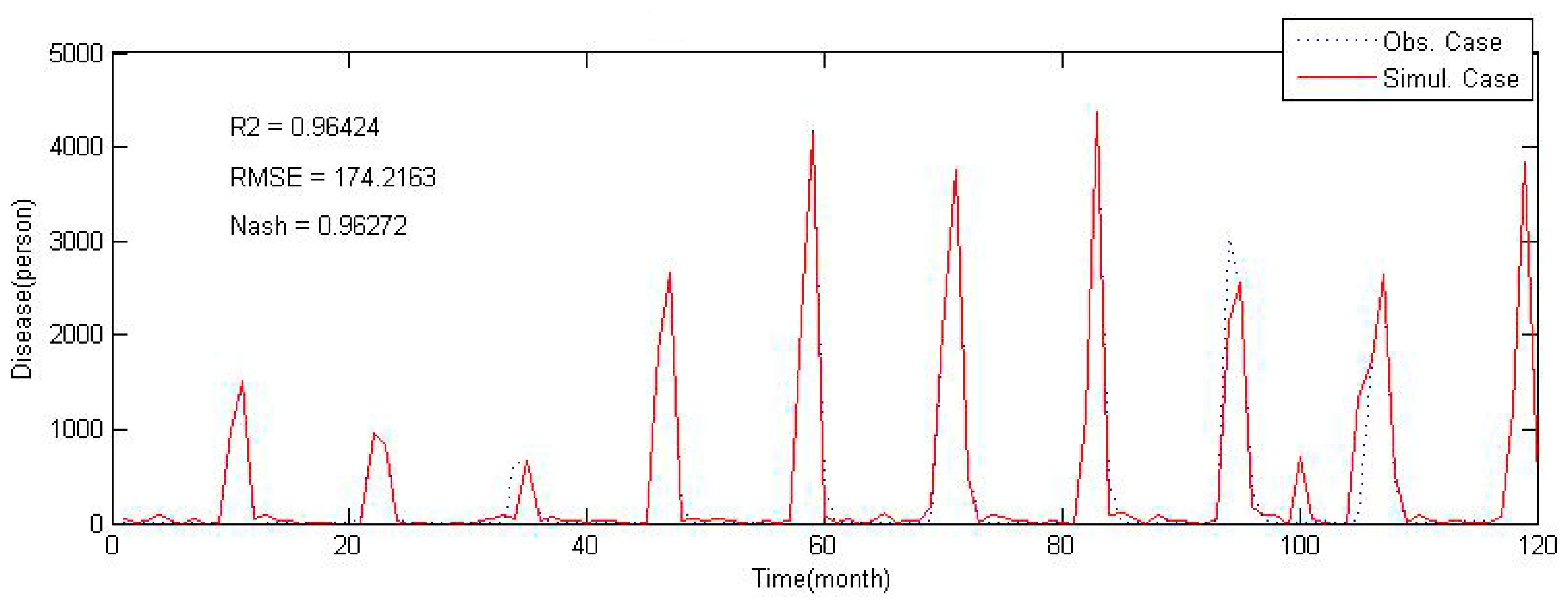
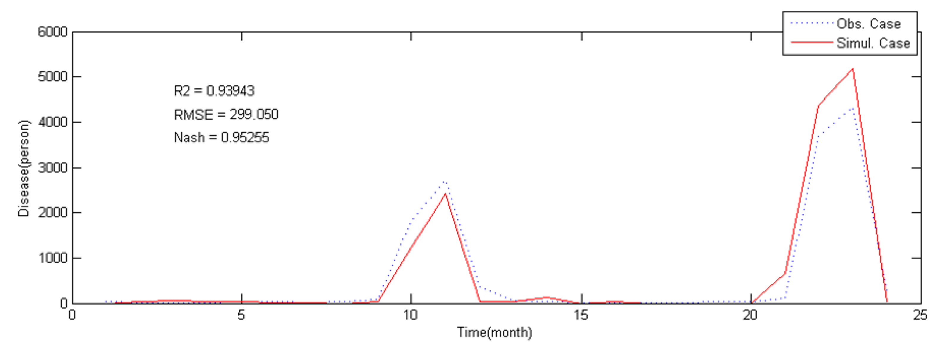
4.2. Validation of the Incidence Model

The scrub typhus incidence mode based on ANN, was evaluated using the incidence data from 2011 to 2012, as shown in Figure 8.

Figure 8. Validation result of scrub typhus incident model.

Figure 8. Validation result of scrub typhus incident model.

Results of evaluation showed R² of 0.94, RMSE of 299, and the Nash-Sutcliffe coefficient of 0.95. Both the calibration and the validation results indicate that selected predictors are mainly responsible in the scrub typhus modeling. The evaluation results of the whole period are shown in Table 2.

Table 2. Evaluation function value of each phase.

E. Func. Period	R2	Nash	RMSE (Person)
Calibration (2001–2010)	0.946	0.963	174
Validation (2011–2012)	0.939	0.953	299

Table 2. Evaluation function value of each phase.

E. Func. Period	R2	Nash	RMSE (Person)
Calibration (2001–2010)	0.946	0.963	174
Validation (2011–2012)	0.939	0.953	299

5. Results and Discussion

This study was conducted for constructing a scrub typhus incidence model with the use of ANN. For this, we selected proper predictors with time-lag (k) from among meteorological factors based on the Granger causality and cross spectral analysis. As shown in Table 1 and Figure 6, scrub typhus is mainly correlated with meteorological factors with 1 month and 4 to 6 month time lags. For example, the mean temperature is correlated when $k=1,3,4$ months, minimum temperature is when $k=3,6$, maximum temperature is when $k=1,3,6$, precipitation is when $k=1,4,6$, and relative humidity and wind speed are when $k=1,6$. Generally, the occurrence of scrub typhus depends on temperature, because its vectors, Trombiculidae mites, are ectothermic insects. Therefore, time lag ($k=1$) correlation between scrub typhus and each temperature are not surprising, because Trombiculidae mite activity depends on temperature. But there are other times lags ($k=3,4\text{ and }6$) for temperature, precipitation, relative humidity and wind speed that seem to be related with the spawning condition. In Korea, Trombiculidae are known to mainly spawn in summer and stop spawning during fall and winter seasons [76] and Trombiculidae spawning rates are increasing with temperature [77]. In particular, the adult Trombiculidae stop their spawning when humidity is low [76]. Therefore, a large time-lag ($k=3,4\text{ and }6$) indicates spawning in summer season ($k=3,4\text{ and }6$ correspond to May, July and August). The wind speed also shows some correlation with scrub typhus, but wind speed was not considered in the previous studies on epidemiology and ecology. Hence, there are no clues as to why or how it has correlation with the scrub typhus occurrence, and further studies are needed in the perspective of ecology of the Trombiculidae life cycle or infection mechanism with wind speed. With this and validation results (Figure 7 and Figure 8) in mind, the proposed incidence model can be used for short-term forecasting of scrub typhus incidences in Korea.

The second thing is the seasonality of meteorological data. The seasonality in the meteorological factors was removed before using them as predictors, otherwise it can cause error in the incidence model predictions. However, there is uncertainty that seasonality will really cause error in the constructed model. Because Granger’s causality or 1 dimensional spectral analysis cannot detect seasonality and correlation, we performed cross-wavelet analysis to visualize these characteristics in time-domain spaces. Following Torrence and Compo [78] and Grinsted et al. [52], we used wavelet transform and selected the frequency scale factor.

Meteorological predictors that have seasonality show 11 to 13 month (approximatively 12 month) cycle correlation for the whole period with 95% confidence inbound, as the bold lined area in Figure 10, but they do not have significant correlation with scrub typhus outbreak events. This means that scrub typhus has its own occurrence cycle and it is weakly correlated with meteorological predictors, which also have their own seasonality (Figure 10), so meteorological data cannot be used as predictors. However, several studies show that meteorological factors are most responsible for scrub typhus in Korea. On the other hand, Figure 9 shows correlation for each year outbreak time with mean temperature, precipitation, relative humidity, and wind speed with 1 to 7 months lag. This strongly suggests that 11 to 13 month seasonality in raw meteorological predictors (Figure 10) can cause spurious correlation, which is mainly affected by the seasonality of meteorological data [79], which are used in the correlation analysis or regression, or even in the network models. Therefore, the study on Scrub typhus modeling, relating to meteorological factors, in Korea should better consider the seasonality of meteorological data.

Figure 9. Cross wavelet analysis results between scrub typhus and processed meteorological predictors (removed seasonality): scrub typhus with (a) mean temperature; (b) precipitation; (c) relative humidity; (d) wind speed; (e) duration of sunshine; and (f) cloud amount; bold line indicates 95% confidence inbound which is statistically significant and white transparency area indicates un-confidence area, and blue to red colors indicate the temporal correlation scale with each color-map index.

Figure 9. Cross wavelet analysis results between scrub typhus and processed meteorological predictors (removed seasonality): scrub typhus with (a) mean temperature; (b) precipitation; (c) relative humidity; (d) wind speed; (e) duration of sunshine; and (f) cloud amount; bold line indicates 95% confidence inbound which is statistically significant and white transparency area indicates un-confidence area, and blue to red colors indicate the temporal correlation scale with each color-map index.

Figure 10. Cross wavelet analysis between scrub typhus and raw meteorological predictors (non-removed seasonality): scrub typhus with (a) mean temperature; (b) precipitation; (c) relative humidity; (d) wind speed; (e) duration of sunshine, and (f) cloud cover; bold line indicates 95% confidence inbound which is statistically significant and white transparency area indicates un-confidence area, and blue to red colors indicate the temporal correlation scale with each color-map index.

Figure 10. Cross wavelet analysis between scrub typhus and raw meteorological predictors (non-removed seasonality): scrub typhus with (a) mean temperature; (b) precipitation; (c) relative humidity; (d) wind speed; (e) duration of sunshine, and (f) cloud cover; bold line indicates 95% confidence inbound which is statistically significant and white transparency area indicates un-confidence area, and blue to red colors indicate the temporal correlation scale with each color-map index.

A limitation of this study is the lack of long time incidence data. Scrub typhus incidence data from 2001 to 2012 years were collected for this study. These 12 years data may suffice to construct the incidence model, but it is difficult to prove if the data are really enough. The incidence of scrub typhus in Korea has significantly increased from average 250 cases per year to average 1,300 cases per year in 1997 to 1998 year and has stabilized at average 3500 cases per year near 2001 to 2005 for [33]. Also, meteorological conditions have actually changed from 2000 onwards [6]. So, the use of data before the 2001 year may cause error in the study. Accordingly we obtained incidence data for 2001 to 2012. Also, the method suggested in this study is clearly a way to construct a prediction model for epidemic diseases which are correlated with meteorological factors. Especially, recent studies suggested that the future meteorological data can be acquired through the climate model with 3 month lead time [80], with maximum 18 month lead time for ENSO [81]. Therefore, the suggested method and model can provide reliable data, which are outbreak time and approximate case number based on meteorological data for the decision maker or agencies of public health.

6. Conclusions

The study clarifies the correlation between monthly meteorological data and scrub typhus incidence and establishes a reliable incidence ANN model. It also shows that the seasonality of meteorological factors affects model prediction in Korea. From the results of this study the following conclusions may be drawn:

(1)

A scrub typhus incidence model with an ANN model is constructed. Based on the correlation between scrub typhus cases and monthly meteorological data, the mean, maximum and minimum temperatures, precipitation, relative humidity, wind speed data were selected as predictors. Also, appropriate time-lags were selected using Granger’s causality and cross spectrum and coherence. The constructed model is validated from 2011 to 2012 and R² is 0.94, RMSE is 299 and Nash efficiency is 0.95, which clearly account for scrub typhus incidence. So, the method and the incidence model suggested in this study can provide reliable data for the decision makers or agencies of public health.

(2)

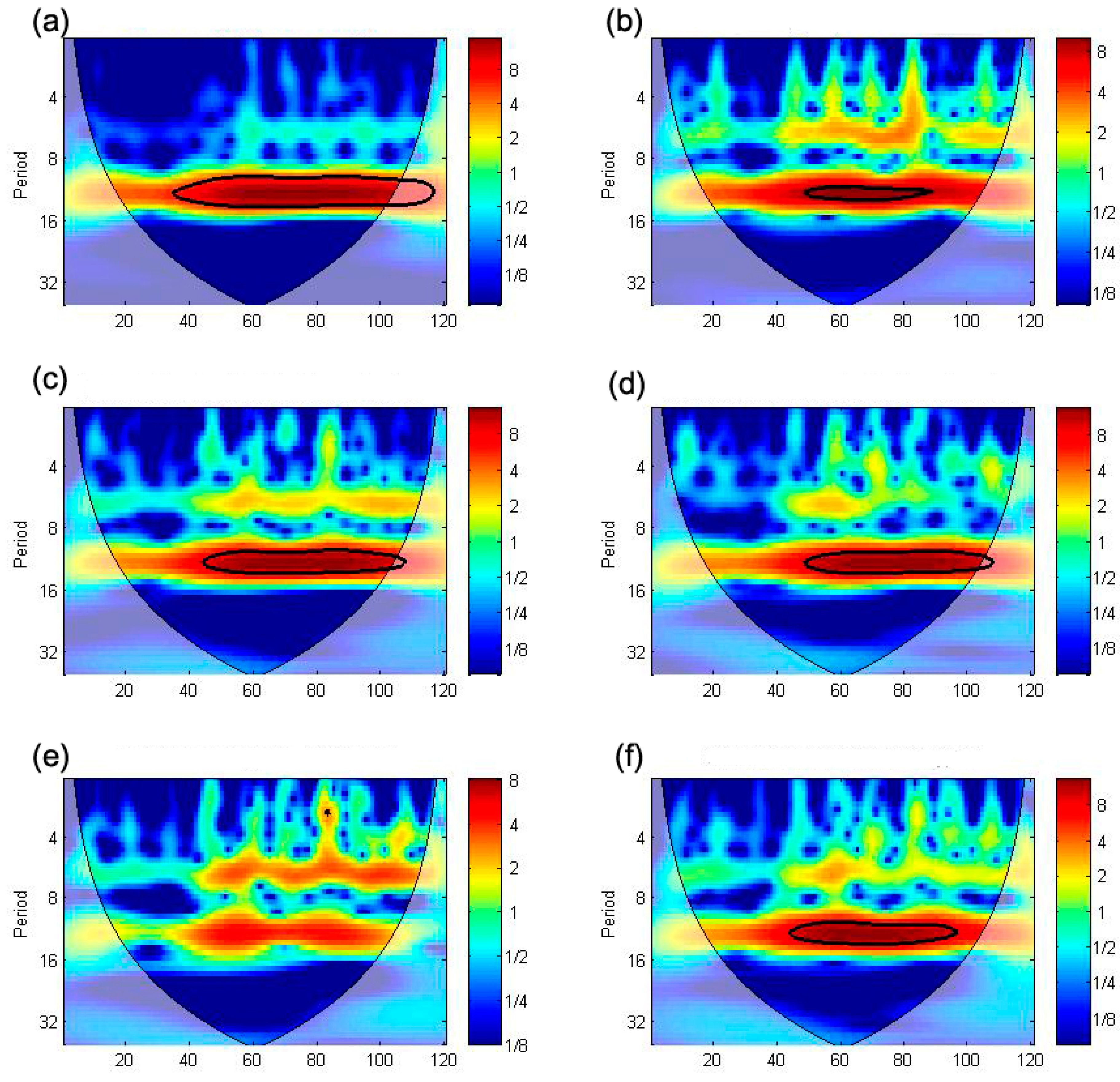
To visualize the seasonality effect in the predictors, cross-wavelet analysis is conducted. Meteorological predictors without seasonality eliminated show a strong 11 to 13 month correlation cycle during the whole period. But the results for predictors with seasonality removed show 1 to 7 month correlation for each year outbreak time with mean temperature, precipitation, relative humidity and wind speed. This suggests that seasonality can affect correlation. This means that any scrub typhus prediction model in Korea should consider seasonality.

References

1. Tsai, P.J.; Yeh, H.C. Scrub typhus islands in the Taiwan area and the association between scrub typhus disease and forest land use and farmer population density: Geographically weighted regression. BMC Infect. Dis. 2013, 13, 1–16. [Google Scholar] [CrossRef] [PubMed]
2. Watt, G.; Parola, P. Scrub typhus and tropical rickettsioses. Curr. Opin. Infect. Dis. 2003, 16, 429–436. [Google Scholar] [CrossRef] [PubMed]
3. Bang, H.A.; Lee, M.J.; Lee, W.C. Comparative research on epidemiological aspects of tsutsugamushi disease (scrub typhus) between Korea and Japan. J. Infect. Dis. 2008, 61, 148–150. (In Japanese) [Google Scholar]
4. Cho, H.W.; Chu, C. The geographical and economical impact of Scrub Typhus, the fastest-growing vector-borne disease in Korea. Osong Public Health Res. Perspect. 2013, 4, 1–3. [Google Scholar] [CrossRef] [PubMed]
5. Jang, J.Y.; Cho, S.H.; Kim, S.Y.; Cho, S.N.; Kim, M.S.; Baek, K.W. Assessment of Climate Change Impact and Preparation of Adaptation Program in Korea; Ministry of Environment: Seoul, Korea, 2003.
6. Choi, Y. Trends on temperature and precipitation extreme events in Korea. J. Korean Geogr. Soc. 2004, 39, 711–721. (In Korean) [Google Scholar]
7. Kalra, S.L.; Rao, K.N. Typhus fevers in Kashmir State. Part II. Murine typhus. Indian J. Med. Res. 1951, 39, 297–302. [Google Scholar] [PubMed]
8. Kelly, D.J.; Fuerst, P.A.; Ching, W.M.; Richards, A.L. Scrub typhus: the geographic distribution of phenotypic and genotypic variants of Orientia tsutsugamushi. Clin. Infect. Dis. 2009, 48, 203–230. [Google Scholar] [CrossRef] [PubMed]
9. Traub, R.; Wisseman, C.L. The ecology of chigger-borne rickettsiosis (scrub typhus). J. Med. Entomol. 1974, 11, 237–303. [Google Scholar] [CrossRef] [PubMed]
10. Kasuya, S. Studies on tsutsugamushi disease in Gifu prefecture. 6. Correlation between number of patients and meteorological elements. Kansenshogaku zasshi. J. Jpn. Assoc. Infect. Dis. 1995, 69, 1110–1117. (In Japanese) [Google Scholar]
11. Kawamura, A.; Tanaka, H.; Takamura, A. Tsutsugamushi Disease: An Overview; University of Tokyo Press: Tokyo, Japan, 1995. [Google Scholar]
12. Zhang, S.; Gao, Q. Predicting the incidence of typhus by regression analysis in Shijiazhuang City. Chin. J. Zoonoses 2011, 6, 1–9. [Google Scholar]
13. Li, T.; Yang, Z.; Dong, Z.; Wang, M. Meteorological factors and risk of scrub typhus in Guangzhou, Southern China, 2006–2012. BMC Infect. Dis. 2014, 14, 1–8. [Google Scholar] [CrossRef] [PubMed]
14. Gage, K.L.; Burkot, T.R.; Eisen, R.J.; Hayes, E.B. Climate and vectorborne diseases. Amer. J. Prev. Med. 2008, 35, 436–450. [Google Scholar] [CrossRef] [PubMed]
15. Gubler, D.J.; Reiter, P.; Ebi, K.L.; Yap, W.; Nasci, R.; Patz, J.A. Climate variability and change in the United States: Potential impacts on vector-and rodent-borne diseases. Environ. Health Perspect. 2001, 109, 223–233. [Google Scholar] [CrossRef] [PubMed]
16. Costello, A.; Abbas, M.; Allen, A.; Ball, S.; Bell, S.; Bellamy, R.; Patterson, C. Managing the health effects of climate change. Lancet 2009, 373, 1693–1733. [Google Scholar] [CrossRef]
17. Greer, A.; Ng, V.; Fisman, D. Climate change and infectious diseases in North America: The road ahead. Can. Med. Assoc. J. 2008, 178, 715–722. [Google Scholar]
18. Patz, J.A.; Campbell-Lendrum, D.; Holloway, T.; Foley, J.A. Impact of regional climate change on human health. Nature 2005, 438, 310–317. [Google Scholar] [CrossRef] [PubMed]
19. Singh, R.B.; Hales, S.; de Wet, N.; Raj, R.; Hearnden, M.; Weinstein, P. The influence of climate variation and change on diarrheal disease in the Pacific Islands. Environ. Health Perspect. 2001, 109, 155–159. [Google Scholar] [CrossRef] [PubMed]
20. Tanser, F.C.; Sharp, B.; le Sueur, D. Potential effect of climate change on malaria transmission in Africa. Lancet 2003, 362, 1792–1798. [Google Scholar] [CrossRef]
21. Chang, K.; Lee, N.Y.; Ko, W.C.; Tsai, J.J.; Lin, W.R.; Chen, T.C.; Chen, Y.H. Identification of factors for physicians to facilitate the early differential diagnosis of scrub typhus, murine typhus and Q fever from the dengue fever in Taiwan. J. Microbiol. Immunol. Infect. 2014, 14. [Google Scholar] [CrossRef] [PubMed]
22. Chen, M.J.; Lin, C.Y.; Wu, Y.T.; Wu, P.C.; Lung, S.C.; Su, H.J. Effects of extreme precipitation to the distribution of infectious diseases in Taiwan, 1994–2008. PLoS ONE 2012, 7. [Google Scholar] [CrossRef] [PubMed]
23. Haines, A.; Kovats, R.S.; Campbell-Lendrum, D.; Corvalan, C. Climate change and human health: Impacts, vulnerability and public health. Public Health 2006, 120, 585–596. [Google Scholar] [CrossRef] [PubMed]
24. Kim, J.H.; Cheong, H.K. Impacts of Climate on the Incidence of Scrub Typhus. Epidemiology 2009, 20, 202–203. [Google Scholar] [CrossRef]
25. Kim, S.H.; Jang, J.Y. Correlations between Climate Change-Related Infectious Diseases and Meteorological Factors in Korea. J. Prev. Med. Public Health 2010, 43, 436–444. (In Korean) [Google Scholar] [CrossRef] [PubMed]
26. Moosa, S. Adaptation measures for human health in response to climate change in Maldives. Regional Health Forum 2008, 12, 49–55. [Google Scholar]
27. Ostfeld, R.S.; Keesing, F. Biodiversity series: the function of biodiversity in the ecology of vector-borne zoonotic diseases. Can. J. Zool. 2000, 78, 2061–2078. [Google Scholar] [CrossRef]
28. Li, X.; Gao, L.; Dai, L.; Zhang, G.; Zhuang, X.; Wang, W.; Zhao, Q. Understanding the relationship among urbanization, climate change and human health: A case study in Xiamen. Int. J. Sustain. Dev. World Ecol. 2010, 17, 304–310. [Google Scholar] [CrossRef]
29. Kuo, C.C.; Huang, J.L.; Ko, C.Y.; Lee, P.F.; Wang, H.C. Spatial analysis of scrub typhus infection and its association with environmental and socioeconomic factors in Taiwan. Acta Tropica 2011, 120, 52–58. [Google Scholar] [CrossRef] [PubMed]
30. Crippen, R.E. Calculating the vegetation index faster. Remote Sens. Environ. 1990, 34, 71–73. [Google Scholar] [CrossRef]
31. Yang, L.P.; Liu, J.; Wang, X.J.; Ma, W.; Jia, C.X.; Jiang, B.F. Effects of meteorological factors on scrub typhus in a temperate region of China. Epidemiol. Infect. 2014, 142, 2217–2226. [Google Scholar] [CrossRef] [PubMed]
32. Chang, W.H. Tsutsugamushi Disease in Korea; Seohung Press Inc.: Seoul, Korea, 1994. (In Korean) [Google Scholar]
33. KCDC (Korea Centers for Disease Control & Prevention). Infectious Disease Study. Available online: http://www.cdc.go.kr/ (accessed on 15 May 2014).
34. Lee, S.H.; Lee, Y.S.; Lee, I.Y.; Lim, J.W.; Shin, H.K.; Yu, J.R.; Sim, S. Monthly occurrence of vectors and reservoir rodents of scrub typhus in an endemic area of Jeollanam-do, Korea. Korean J. Parasitol. 2012, 50, 327–331. (In Korean) [Google Scholar] [CrossRef] [PubMed]
35. World Health Organization. Frequently Asked Questions: Scrub Typhus 2009; WHO: Bangkok, Thailand, 2009; Available online: http://www.searo.who.int/LinkFiles/CDS_faq_Scrub_Typhus.pdf (accessed on 5 December 2014).
36. Chae, J.S.; Adjemian, J.Z.; Kim, H.C.; Ko, S.; Klein, T.A.; Foley, J. Predicting the emergence of tick-borne infections based on climatic changes in Korea. Vector-Borne Zoonotic Dis. 2008, 8, 265–276. [Google Scholar] [CrossRef] [PubMed]
37. Yoon, S.J.; Oh, I.H.; Seo, H.Y.; Kim, E.J. Measuring the burden of disease due to climate change and developing a forecast model in South Korea. Public Health 2014, 128, 725–733. [Google Scholar] [CrossRef] [PubMed]
38. Chung, Y.S.; Yoon, M.B.; Kim, H.S. On climate variations and changes observed in South Korea. Clim. Chang. 2004, 66, 151–161. [Google Scholar] [CrossRef]
39. Noh, J.H.; Shin, Y.H.; Ju, Y.R. Nationwide surveillance of chigger mites, as the vector of scrub typhus. Public Health Wkly. Rep. KCDC 2014, 7, 1146–1148. (In Korean) [Google Scholar]
40. Kim, S.W.; Kim, Y.H. Spatial analysis modeling on scrub typhus disease occurrence in Korea. J. Korean Cartogr. Assoc. 2014, 14, 41–54. [Google Scholar] [CrossRef]
41. Kong, W.S.; Shin, E.H.; Lee, H.I.; Hwang, T.S.; Kim, H.H.; Lee, N.Y.; Yoon, K.H. Time-spatial distribution of scrub typhus and its environmental ecology. J. Korean Geogr. Soc. 2007, 42, 863–878. (In Korean) [Google Scholar]
42. Park, S.J. Characteristic Relating to the Occurrence of Tsutsugamushi Disease Using GIS. Ph.D. Dissertation, The Graduate School of Inje University, Gimhae, Korea, 2008. [Google Scholar]
43. Jin, H.S.; Chu, C.; Han, D.Y. Spatial distribution analysis of scrub typhus in Korea. Osong Public Health Res. Perspect. 2013, 4, 4–15. [Google Scholar] [CrossRef] [PubMed]
44. KMA (Korea Meteorological Administration). Available online: http://www.cdc.go.kr/ (accessed on 15 August 2015).
45. Granger, C.W.J. Investigating causal relations by econometric models and cross-spectral methods. Econometrica 1969, 37, 424–438. [Google Scholar] [CrossRef]
46. Granger, C.W.J. Essays in Econometrics: The Collected Papers of Clive W.J. Granger; Cambridge University Press: Cambridge, UK, 2001. [Google Scholar]
47. Ding, M.; Chen, Y.; Bressler, S. Granger causality: Basic theory and application to neuroscience. In Handbook of Time Series Analysis; Wiley: Wienheim, Germany, 2006. [Google Scholar]
48. Ricker, D.W. Echo Signal Processing; Springer: New York, NY, USA, 2003. [Google Scholar]
49. Hies, T.; Treffeisen, R.; Sebald, L.; Reimer, E. Spectral analysis of air pollutants. Part 1: Elemental carbon time series. Atmos. Environ. 2000, 34, 3495–3502. [Google Scholar] [CrossRef]
50. Zhukov, M. Analysis of interconnection between central nervous and cardiovascular systems. Electron. Comm. 2014, 19, 26–36. [Google Scholar]
51. Jevrejeva, S.; Moore, J.C.; Grinsted, A. Influence of the Arctic Oscillation and El Niño-Southern Oscillation (ENSO) on ice conditions in the Baltic Sea: The wavelet approach. J. Geophys. Res. 2003, 108, 1–11. [Google Scholar] [CrossRef]
52. Grinsted, A.; Moore, J.C.; Jevrejeva, S. Application of the cross wavelet transform and wavelet coherence to geophysical time series. Nonlin. Process. Geophys. 2004, 11, 561–566. [Google Scholar] [CrossRef]
53. Lin, J.; Qu, L. Feature extraction based on Morlet wavelet and its application for mechanical fault diagnosis. J. Sound Vib. 2000, 234, 135–148. [Google Scholar] [CrossRef]
54. Kihoro, J.M.; Otieno, R.O.; Wafula, C. Seasonal time series forecasting: A comparative study of ARIMA and ANN models. Afr. J. Sci. Technol. 2004, 5, 41–49. [Google Scholar] [CrossRef]
55. Fukushima, K. Neocognitron: A self-organizing neural network model for a mechanism of pattern recognition unaffected by shift in position. Biol. Cybern. 1980, 36, 93–202. [Google Scholar] [CrossRef]
56. Hopfield, J.J. Neural networks and physical systems with emergent collective computational abilities. Proc. Natl. Acad. Sci. USA 1982, 79, 2554–2558. [Google Scholar] [CrossRef] [PubMed]
57. Rosenblatt, F. The perceptron: a probabilistic model for information storage and organization in the brain. Psychol. Rev. 1958, 65, 386–408. [Google Scholar] [CrossRef] [PubMed]
58. Haykin, S. Neural Networks: A Comprehensive Foundation; Prentice Hall: Upper Saddle River, NJ, USA, 1999. [Google Scholar]
59. Battiti, R. Accelerated backpropagation learning: Two optimization methods. Complex Syst. 1989, 3, 331–342. [Google Scholar]
60. Lera, G.; Pinzolas, M. Neighborhood based Levenberg-Marquardt algorithm for neural network training. IEEE Trans. Neural Netw. 2002, 13, 1200–1203. [Google Scholar] [CrossRef] [PubMed]
61. Ngia, L.S.; Sjoberg, J. Efficient training of neural nets for nonlinear adaptive filtering using a recursive Levenberg-Marquardt algorithm. IEEE Trans. Signal Process. 2000, 48, 1915–1927. [Google Scholar] [CrossRef]
62. Kim, D.M.; Lee, Y.M.; Back, J.H.; Yang, T.Y.; Lee, J.H.; Song, H.J.; Park, M.Y. A serosurvey of Orientia tsutsugamushi from patients with scrub typhus. Clin. Microbiol. Infect. 2010, 16, 447–451. [Google Scholar] [CrossRef] [PubMed]
63. Payne, K.S.; Klein, T.A.; Otto, J.L.; Kim, H.C.; Chong, S.T.; Ha, S.J.; Song, J.W. Seasonal and environmental determinants of leptospirosis and scrub typhus in small mammals captured at a U.S. military training site (Dagmar North), Republic of Korea, 2001–2004. Mil. Med. 2009, 174, 1061–1067. [Google Scholar] [CrossRef] [PubMed]
64. Bernstein, J. Seasonality: Systems, Strategies, and Signals; John Wiley & Sons: New York, NY, USA, 1998; Volume 13. [Google Scholar]
65. Briët, O.J.; Vounatsou, P.; Gunawardena, D.M.; Galappaththy, G.N.; Amerasinghe, P.H. Temporal correlation between malaria and rainfall in Sri Lanka. Malar. J. 2008, 7, 1–14. [Google Scholar] [CrossRef] [PubMed]
66. Kawale, J.; Chatterjee, S.; Kumar, A.; Liess, S.; Steinbach, M.; Kumar, V. Anomaly Construction in Climate Data: Issues and Challenges. In Proceedings of the CIDU Conference; Mountain View, CA, USA, 2011; pp. 189–203. [Google Scholar]
67. Wakaura, M.; Ogata, Y. A time series analysis on the seasonality of air temperature anomalies. Meteorol. Appl. 2007, 14, 425–434. [Google Scholar] [CrossRef]
68. Song, H.J.; Kim, K.H.; Kim, S.C.; Hong, S.S.; Ree, H.I. Population density of chigger mites, the vector of tsutsugamushi disease in Chollanam-do, Korea. Korean J. Parasitol. 1996, 34, 27–33. (In Korean) [Google Scholar] [CrossRef] [PubMed]
69. Park, S.Y.; Han, D.K. Reviews in medical geography: Spatial epidemiology of vector-borne diseases. J. Korean Geogr. Soc. 2012, 47, 677–699. [Google Scholar]
70. Yoo, S.J.; Lee, W.K.; Oh, S.H.; Byun, J.Y. Vulnerability assessment for public health to climate change using spatio-temporal information based on GIS. J. Korean Spat. Inf. Soc. 2012, 20, 13–24. (In Korean) [Google Scholar] [CrossRef]
71. Heaton, J. Introduction to Neural Networks with Java; Heaton Research, Inc.: Chesterfield, MO, USA, 2008. [Google Scholar]
72. Gujarati, D.N. Basic Econometrics; Tata McGraw-Hill Education: Noida, UP, India, 2012. [Google Scholar]
73. Hyndman, R.J.; Khandakar, Y. Automatic Time Series for Forecasting: The Forecast Package for R (No. 6/07); Monash University: Victoria, Australia, 2007. [Google Scholar]
74. Nash, J.E.; Sutcliffe, J.V. River flow forecasting through conceptual models part I—A discussion of principles. J. Hydrol. 1970, 10, 282–290. [Google Scholar] [CrossRef]
75. Yang, L.P.; Liang, S.Y.; Wang, X.J.; Li, X.J.; Wu, Y.L.; Ma, W. Burden of disease measured by disability-adjusted life years and a disease forecasting time series model of scrub typhus in Laiwu, China. PLoS Negl. Trop. Dis. 2015, 9, 1–9. [Google Scholar] [CrossRef] [PubMed]
76. Ree, H.I. Medical Entomology, 3rd ed.; Ko-Moon Co.: Seoul, Korea, 1994. (In Korean) [Google Scholar]
77. Van Peenen, P.F.; Lien, J.C.; Santana, F.J.; See, R. Correlation of chigger abundance with temperature at a hyperendemic focus of scrub typhus. J. Parasitol. 1976, 62, 653–654. [Google Scholar] [CrossRef] [PubMed]
78. Torrence, C.; Compo, G.P. A practical guide to wavelet analysis. Bull. Amer. Meteorol. Soc. 1998, 79, 61–78. [Google Scholar] [CrossRef]
79. Hamzaçebi, C. Improving artificial neural networks’ performance in seasonal time series forecasting. Inf. Sci. 2008, 178, 4550–4559. [Google Scholar] [CrossRef]
80. Palmer, T.; Andersen, U.; Cantelaube, P.; Davey, M.; Deque, M.; Doblas-Reyes, F.J.; Thomsen, M.C. Development of a European multi-model ensemble system for seasonal to inter-annual prediction (DEMETER). Bull. Am. Meteorol. Soc. 2004, 85, 853–872. [Google Scholar] [CrossRef]
81. Luo, L.; Wood, E.F.; Pan, M. Bayesian merging of multiple climate model forecasts for seasonal hydrological predictions. J. Geophys. Res. Atmos. 2007, 112, 1350–1363. [Google Scholar] [CrossRef]