Exploring Spatial Trends and Influencing Factors for Gastric Cancer Based on Bayesian Statistics: A Case Study of Shanxi, China

Abstract
:1. Introduction
2. Materials and Methodologies
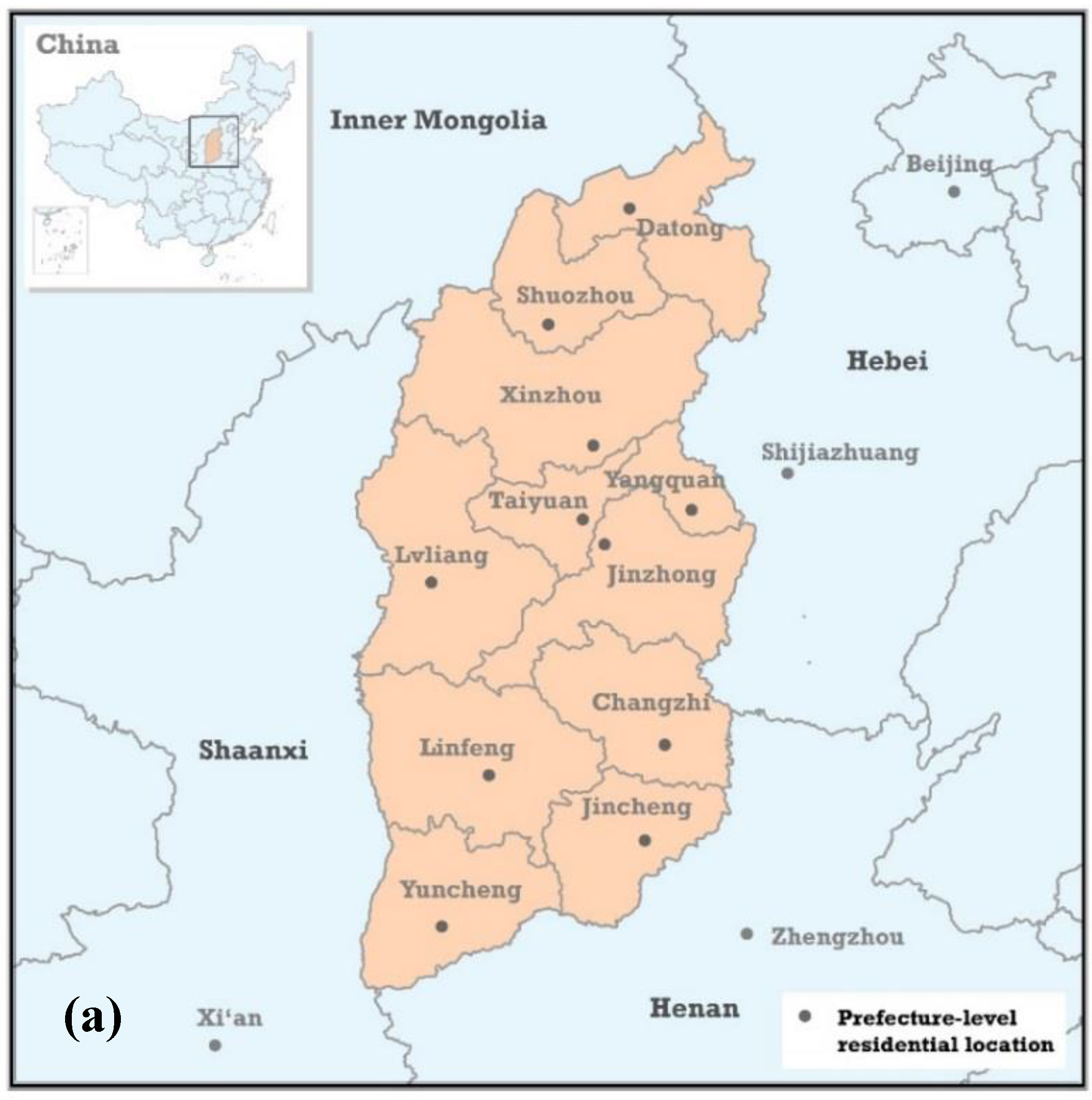
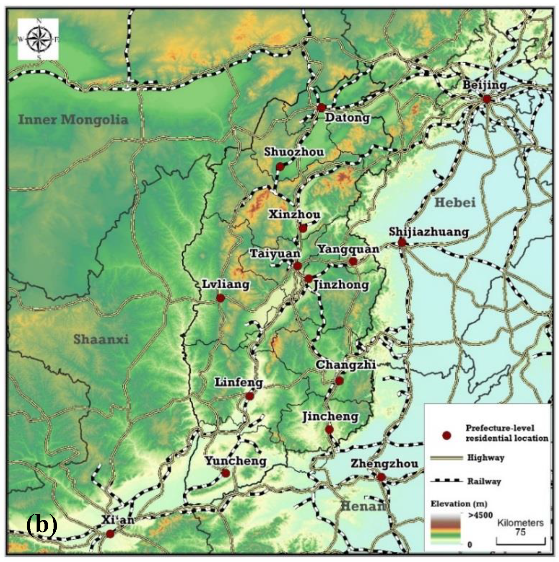
2.1. Study Materials
2.1.1. Diagnosed Patients
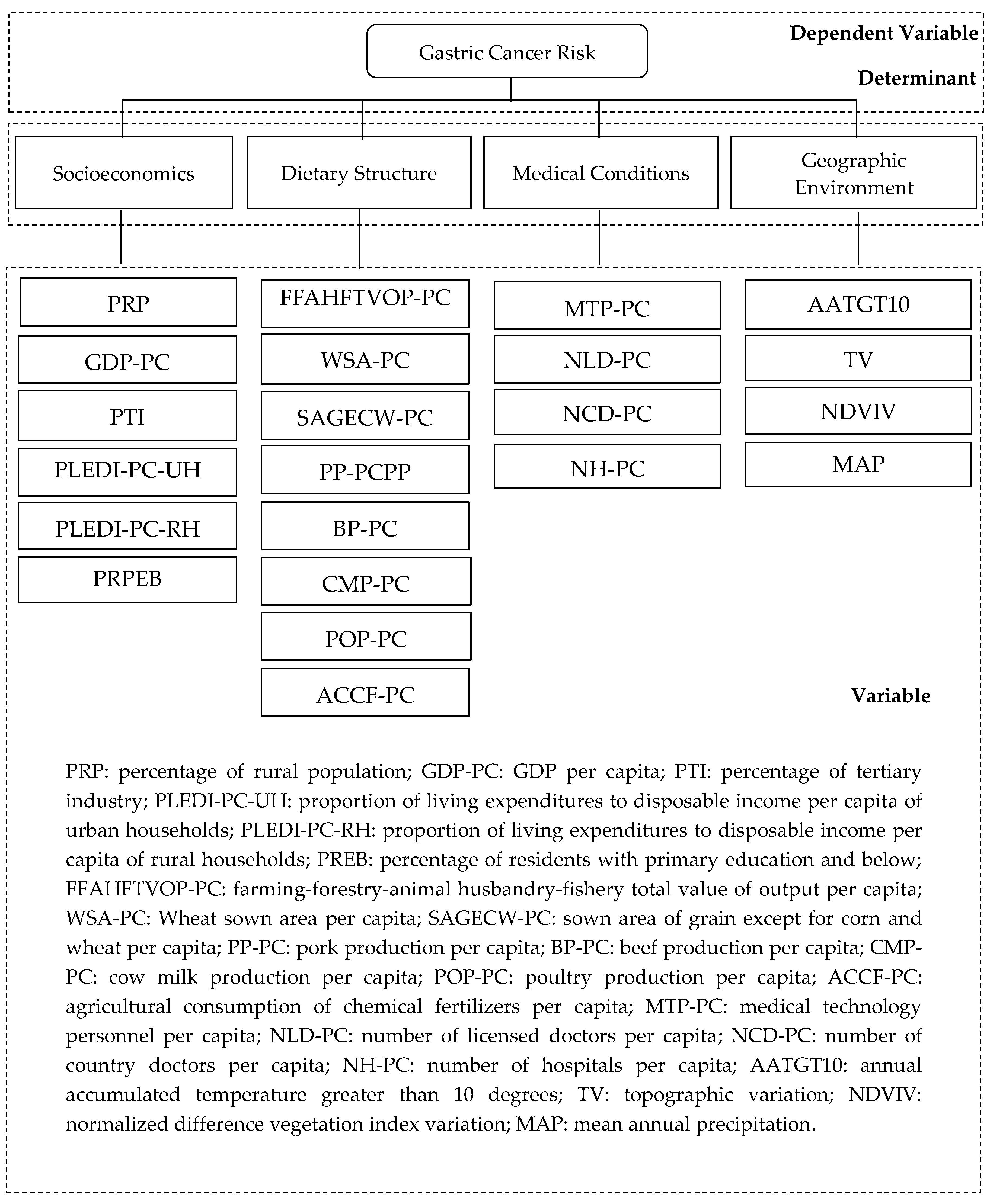
2.1.2. Determinant Variables
2.2. Methodologies
2.2.1. Bayesian Spatial Statistical Model Integrated with a Selection Probability Model
2.2.2. Bayesian Lasso Regression Model
3. Results
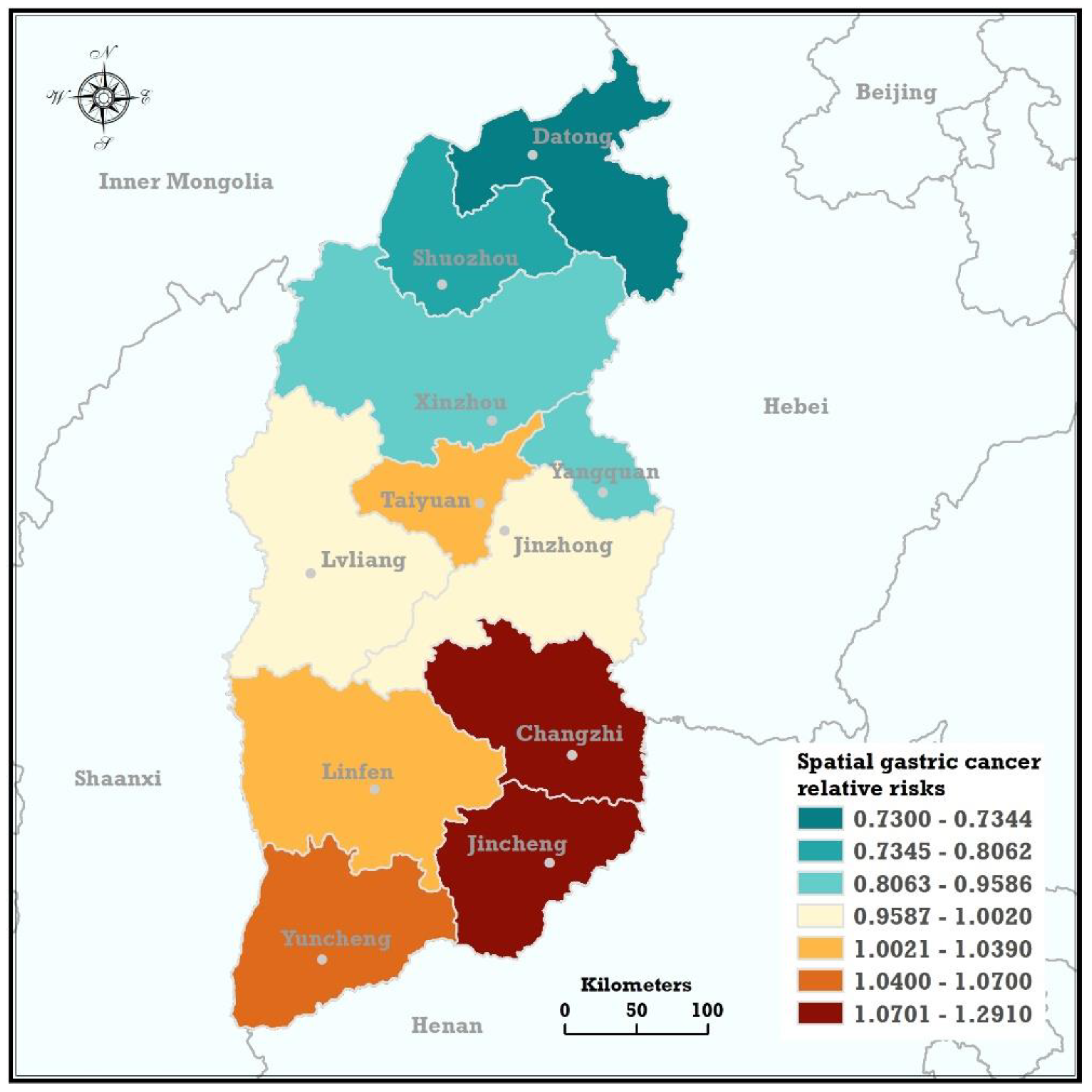
3.1. Spatial Trends
3.2. Verification of Spatial Trends
3.3. Influencing Factors
3.3.1. Univariable Analysis
3.3.2. Multivariable Regression Results
4. Discussion
5. Conclusions
Author Contributions
Acknowledgements
Conflicts of interest
References
- Van Cutsem, E.; Sagaert, X.; Topal, B.; Haustermans, K.; Prenen, H. Gastric cancer. Lancet 2016, 388, 2654–2664. [Google Scholar] [CrossRef]
- Ferlay, J.; Steliarovafoucher, E.; Lortettieulent, J.; Rosso, S.; Coebergh, J.W.; Comber, H.; Forman, D.; Bray, F. Cancer incidence and mortality patterns in Europe: Estimates for 40 countries in 2012. Eur. J. Cancer 2013, 49, 1374–1403. [Google Scholar] [CrossRef] [PubMed] [Green Version]
- Ge, S.; Xia, X.; Ding, C.; Zhen, B.; Zhou, Q.; Feng, J.; Yuan, J.; Chen, R.; Li, Y.; Ge, Z. A proteomic landscape of diffuse-type gastric cancer. Nat. Commun. 2018, 9, 1012. [Google Scholar] [CrossRef] [PubMed] [Green Version]
- Chen, W.; Zheng, R.; Baade, P.D.; Zhang, S.; Zeng, H.; Bray, F.; Jemal, A.; Yu, X.Q.; He, J. Cancer statistics in China, 2015. CA Cancer J. Clin. 2016, 66, 115–132. [Google Scholar] [CrossRef] [PubMed]
- Nie, Y.; Wu, K.; Yu, J.; Liang, Q.; Cai, X.; Shang, Y.; Zhou, J.; Pan, K.; Sun, L.; Fang, J. A global burden of gastric cancer: The major impact of China. Expert Rev. Gastroenterol. Hepatol. 2017, 11, 651–661. [Google Scholar] [CrossRef] [PubMed]
- Zong, L.; Abe, M.; Seto, Y.; Ji, J. The challenge of screening for early gastric cancer in China. Lancet 2016, 388, 2606. [Google Scholar] [CrossRef]
- Soerjomataram, I.; Lortettieulent, J.; Parkin, D.M.; Ferlay, J.; Mathers, C.; Forman, D.; Bray, F. Global burden of cancer in 2008: A systematic analysis of disability-adjusted life-years in 12 world regions. Lancet 2012, 380, 1840–1850. [Google Scholar] [CrossRef]
- Ferro, A.; Peleteiro, B.; Malvezzi, M.; Bosetti, C.; Bertuccio, P.; Levi, F.; Negri, E.; La, V.C.; Lunet, N. Worldwide trends in gastric cancer mortality (1980–2011), with predictions to 2015, and incidence by subtype. Eur. J. Cancer 2014, 50, 1330–1344. [Google Scholar] [CrossRef] [PubMed]
- Huang, H.Y.; Shi, J.F.; Guo, L.W.; Zhu, X.Y.; Wang, L.; Liao, X.Z.; Liu, G.X.; Bai, Y.N.; Mao, A.Y.; Ren, J.S. Expenditure and financial burden for common cancers in China: A hospital-based multicentre cross-sectional study. Lancet 2016, 388, S10. [Google Scholar] [CrossRef]
- Leung, W.K.; Wu, M.S.; Kakugawa, Y.; Kim, J.J.; Yeoh, K.G.; Goh, K.L.; Wu, K.C.; Wu, D.C.; Sollano, J.; Kachintorn, U. Screening for gastric cancer in Asia: Current evidence and practice. Lancet Oncol. 2008, 9, 279–287. [Google Scholar] [CrossRef]
- Zali, H.; Rezaeitavirani, M.; Azodi, M. Gastric cancer: Prevention, risk factors and treatment. Gastroenterol. Hepatol. Bed Bench 2011, 4, 175–185. [Google Scholar] [PubMed]
- Fock, K.M.; Talley, N.; Moayyedi, P.; Hunt, R.; Azuma, T.; Sugano, K.; Xiao, S.D.; Lam, S.K.; Goh, K.L.; Chiba, T. Asia-Pacific consensus guidelines on gastric cancer prevention. J. Gastroenterol. Hepatol. 2008, 23, 351–365. [Google Scholar] [CrossRef] [PubMed]
- Karimi, P.; Islami, F.; Anandasabapathy, S.; Freedman, N.D.; Kamangar, F. Gastric cancer: Descriptive epidemiology, risk factors, screening, and prevention. Cancer Epidemiol. Biomark. Prev. 2014, 23, 700–713. [Google Scholar] [CrossRef] [PubMed]
- Howlader, N.; Noone, A.; Krapcho, M.; Garshell, J.; Neyman, N.; Altekruse, S.; Kosary, C.; Yu, M.; Ruhl, J.; Tatalovich, Z. SEER Cancer Statistics Review, 1975–2010 (Based on the November 2012 SEER data submission, posted to the SEER web site, April 2013). Bethesda MD Natl. Cancer Inst. 2013, 24, 1–48. [Google Scholar]
- Kelley, J.R.; Duggan, J.M. Gastric cancer epidemiology and risk factors. J. Clin. Epidemiol. 2003, 56, 1–9. [Google Scholar] [CrossRef]
- Brown, L.M.; Devesa, S.S. Epidemiologic trends in esophageal and gastric cancer in the United States. Surg. Oncol. Clin. N. Am. 2002, 11, 235–256. [Google Scholar] [CrossRef]
- Ladeiras-Lopes, R.; Pereira, A.K.; Nogueira, A.; Pinheiro-Torres, T.; Pinto, I.; Santos-Pereira, R.; Lunet, N. Smoking and gastric cancer: Systematic review and meta-analysis of cohort studies. Cancer Causes Control 2008, 19, 689–701. [Google Scholar] [CrossRef] [PubMed]
- Shakeri, R.; Malekzadeh, R.; Etemadi, A.; Nasrollahzadeh, D.; Abedi-Ardekani, B.; Khosnia, M.; Islami, F.; Pourshams, A.; Pawilta, M.; Boffetta, P. Association of tooth loss and oral hygiene with risk of gastric adenocarcinoma. Cancer Prev. Res. 2013. [Google Scholar] [CrossRef] [PubMed]
- Freedman, N.D.; Abnet, C.C.; Leitzmann, M.F.; Mouw, T.; Subar, A.F.; Hollenbeck, A.R.; Schatzkin, A. A prospective study of tobacco, alcohol, and the risk of esophageal and gastric cancer subtypes. Am. J. Epidemiol. 2007, 165, 1424–1433. [Google Scholar] [CrossRef] [PubMed]
- Cook, M.B.; Kamangar, F.; Whiteman, D.C.; Freedman, N.D.; Gammon, M.D.; Bernstein, L.; Brown, L.M.; Risch, H.A.; Ye, W.; Sharp, L. Cigarette smoking and adenocarcinomas of the esophagus and esophagogastric junction: A pooled analysis from the international BEACON consortium. J. Natl. Cancer Inst. 2010, 102, 1344–1353. [Google Scholar] [CrossRef] [PubMed]
- Nishino, Y.; Inoue, M.; Tsuji, I.; Wakai, K.; Nagata, C.; Mizoue, T.; Tanaka, K.; Tsugane, S. Tobacco smoking and gastric cancer risk: An evaluation based on a systematic review of epidemiologic evidence among the Japanese population. Jpn. J. Clin. Oncol. 2006, 36, 800–807. [Google Scholar] [CrossRef] [PubMed]
- Sung, N.; Choi, K.; Park, E.; Park, K.; Lee, S.; Lee, A.; Choi, I.; Jung, K.; Won, Y.; Shin, H. Smoking, alcohol and gastric cancer risk in Korean men: The National Health Insurance Corporation Study. Br. J. Cancer 2007, 97, 700–704. [Google Scholar] [CrossRef] [PubMed]
- Mohebtash, M. Helicobacter pylori and its effects on human health and disease. Arch. Iran. Med. 2011, 14, 192–199. [Google Scholar]
- Helicobacter and Cancer Collaborative Group. Gastric cancer and Helicobacter pylori: A combined analysis of 12 case control studies nested within prospective cohorts. Gut 2001, 49, 347–353. [Google Scholar] [CrossRef]
- Shiota, S.; Suzuki, R.; Yamaoka, Y. The significance of virulence factors in Helicobacter pylori. J. Dig. Dis. 2013, 14, 341–349. [Google Scholar] [CrossRef] [PubMed]
- Huang, J.Q.; Zheng, G.F.; Sumanac, K.; Irvine, E.J.; Hunt, R.H. Meta-analysis of the relationship between cagA seropositivity and gastric cancer. Gastroenterology 2003, 125, 1636–1644. [Google Scholar] [CrossRef] [PubMed]
- Yoshida, T.; Kato, J.; Inoue, I.; Yoshimura, N.; Deguchi, H.; Mukoubayashi, C.; Oka, M.; Watanabe, M.; Enomoto, S.; Niwa, T. Cancer development based on chronic active gastritis and resulting gastric atrophy as assessed by serum levels of pepsinogen and Helicobacter pylori antibody titer. Int. J. Cancer 2014, 134, 1445–1457. [Google Scholar] [CrossRef] [PubMed]
- You, W.-C.; Brown, L.M.; Zhang, L.; Li, J.-Y.; Jin, M.-L.; Chang, Y.-S.; Ma, J.-L.; Pan, K.-F.; Liu, W.-D.; Hu, Y. Randomized double-blind factorial trial of three treatments to reduce the prevalence of precancerous gastric lesions. J. Natl. Cancer Inst. 2006, 98, 974–983. [Google Scholar] [CrossRef] [PubMed]
- Wong, B.C.-Y.; Lam, S.K.; Wong, W.M.; Chen, J.S.; Zheng, T.T.; Feng, R.E.; Lai, K.C.; Hu, W.H.C.; Yuen, S.T.; Leung, S.Y. Helicobacter pylori eradication to prevent gastric cancer in a high-risk region of China: A randomized controlled trial. JAMA 2004, 291, 187–194. [Google Scholar] [CrossRef] [PubMed]
- Sung, J.J.; Lin, S.R.; Ching, J.Y.; Zhou, L.Y.; To, K.F.; Wang, R.T.; Leung, W.K.; Enders, K.; Lau, J.Y.; Lee, Y.T. Atrophy and intestinal metaplasia one year after cure of H. pylori infection: A prospective, randomized study. Gastroenterology 2000, 119, 7–14. [Google Scholar] [CrossRef] [PubMed]
- Leung, W.; Lin, S.; Ching, J.; To, K.; Ng, E.; Chan, F.; Lau, J.; Sung, J. Factors predicting progression of gastric intestinal metaplasia: Results of a randomised trial on Helicobacter pylori eradication. Gut 2004, 53, 1244–1249. [Google Scholar] [CrossRef] [PubMed]
- Marmot, M.; Atinmo, T.; Byers, T.; Chen, J.; Hirohata, T.; Jackson, A.; James, W.; Kolonel, L.; Kumanyika, S.; Leitzmann, C. Food, Nutrition, Physical Activity, and the Prevention of Cancer: A Global Perspective; American Institute for Cancer Research: Washington, DC, USA, 2007. [Google Scholar]
- Kobayashi, M.; Tsubono, Y.; Sasazuki, S.; Sasaki, S.; Tsugane, S. Vegetables, fruit and risk of gastric cancer in Japan: A 10-year follow-up of the JPHC study Cohort I. Int. J. Cancer 2002, 102, 39–44. [Google Scholar] [CrossRef] [PubMed] [Green Version]
- Gao, Y.; Hu, N.; Han, X.Y.; Ding, T.; Giffen, C.; Goldstein, A.M.; Taylor, P.R. Risk factors for esophageal and gastric cancers in Shanxi Province, China: A case-control study. Cancer Epidemiol. 2011, 35, e91–e99. [Google Scholar] [CrossRef] [PubMed]
- Shikata, K.; Kiyohara, Y.; Kubo, M.; Yonemoto, K.; Ninomiya, T.; Shirota, T.; Tanizaki, Y.; Doi, Y.; Tanaka, K.; Oishi, Y. A prospective study of dietary salt intake and gastric cancer incidence in a defined Japanese population: The Hisayama study. Int. J. Cancer 2006, 119, 196–201. [Google Scholar] [CrossRef] [PubMed] [Green Version]
- Dungal, N. The special problem of stomach cancer in Iceland: With particular reference to dietary factors. JAMA 1961, 178, 789–798. [Google Scholar] [CrossRef] [PubMed]
- Nagini, S. Carcinoma of the stomach: A review of epidemiology, pathogenesis, molecular genetics and chemoprevention. World J. Gastrointest. Oncol. 2012, 4, 156–169. [Google Scholar] [CrossRef] [PubMed]
- Serafini, M.; Jakszyn, P.; Luján-Barroso, L.; Agudo, A.; Bas Bueno-de-Mesquita, H.; van Duijnhoven, F.J.; Jenab, M.; Navarro, C.; Palli, D.; Boeing, H.; et al. Dietary total antioxidant capacity and gastric cancer risk in the European prospective investigation into cancer and nutrition study. Int. J. Cancer 2012, 131, e544–e554. [Google Scholar] [CrossRef] [PubMed]
- Zhang, Z.; Xu, G.; Ma, M.; Yang, J.; Liu, X. Dietary fiber intake reduces risk for gastric cancer: A meta-analysis. Gastroenterology 2013, 145, 113–120. [Google Scholar] [CrossRef] [PubMed]
- Muñoz, N.; Plummer, M.; Vivas, J.; Moreno, V.; De Sanjosé, S.; Lopez, G.; Oliver, W. A case-control study of gastric cancer in Venezuela. Int. J. Cancer 2001, 93, 417–423. [Google Scholar] [CrossRef] [PubMed] [Green Version]
- Uthman, O.A.; Jadidi, E.; Moradi, T. Socioeconomic position and incidence of gastric cancer: A systematic review and meta-analysis. J. Epidemiol. Commun. Health 2013, 67, 854–860. [Google Scholar] [CrossRef] [PubMed]
- Tran, G.D.; Sun, X.D.; Abnet, C.C.; Fan, J.H.; Dawsey, S.M.; Dong, Z.W.; Mark, S.D.; Qiao, Y.L.; Taylor, P.R. Prospective study of risk factors for esophageal and gastric cancers in the Linxian general population trial cohort in China. Int. J. Cancer 2005, 113, 456–463. [Google Scholar] [CrossRef] [PubMed]
- Islami, F.; Kamangar, F.; Nasrollahzadeh, D.; Aghcheli, K.; Sotoudeh, M.; Abedi-Ardekani, B.; Merat, S.; Nasseri-Moghaddam, S.; Semnani, S.; Sepehr, A. Socio-economic status and oesophageal cancer: Results from a population-based case-control study in a high-risk area. Int. J. Epidemiol. 2009, 38, 978–988. [Google Scholar] [CrossRef] [PubMed]
- Yamaoka, Y.; Kato, M.; Asaka, M. Geographic differences in gastric cancer incidence can be explained by differences between Helicobacter pylori strains. Intern. Med. 2008, 47, 1077–1083. [Google Scholar] [CrossRef] [PubMed]
- Clements, A.C.; Lwambo, N.J.; Blair, L.; Nyandindi, U.; Kaatano, G.; Kinung’Hi, S.; Webster, J.P.; Fenwick, A.; Brooker, S. Bayesian spatial analysis and disease mapping: Tools to enhance planning and implementation of a schistosomiasis control programme in Tanzania. Trop. Med. Int. Health 2006, 11, 490–503. [Google Scholar] [CrossRef] [PubMed]
- Rodrigues, E.C. Bayesian Spatial Models with a Mixture Neighborhood Structure; Academic Press, Inc.: Cambridge, MA, USA, 2012; pp. 88–102. [Google Scholar]
- Karemera, D.; Oguledo, V.I.; Davis, B. A gravity model analysis of international migration to North America. Appl. Econ. 2000, 32, 1745–1755. [Google Scholar] [CrossRef]
- Yan, X.Y.; Wang, W.X.; Gao, Z.Y.; Lai, Y.C. Universal model of individual and population mobility on diverse spatial scales. Nat. Commun. 2017, 8, 1939. [Google Scholar] [CrossRef] [PubMed]
- Besag, J.; York, J.; Mollié, A. Bayesian image restoration, with two applications in spatial statistics. Ann. Inst. Stat. Math. 1991, 43, 1–20. [Google Scholar] [CrossRef]
- Wall, M.M. A close look at the spatial structure implied by the CAR and SAR models. J. Stat. Plan. Inference 2004, 121, 311–324. [Google Scholar] [CrossRef]
- Hans, C. Bayesian lasso regression. Biometrika 2009, 96, 835–845. [Google Scholar] [CrossRef]
- Park, T.; Casella, G. The Bayesian Lasso. Am. Stat. Assoc. 2008, 103, 681–686. [Google Scholar] [CrossRef]
- Tibshirani, R.J. Regression shrinkage and selection via the LASSO. J. R. Stat. Soc. 1996, 58, 267–288. [Google Scholar]
- Lunn, D.J.; Thomas, A.; Best, N.; Spiegelhalter, D. WinBUGS—A Bayesian modelling framework: Concepts, structure, and extensibility. Stat. Comput. 2000, 10, 325–337. [Google Scholar] [CrossRef]
- Salvatier, J.; Wiecki, T.V.; Fonnesbeck, C. PyMC3: Python Probabilistic Programming Framework; Astrophysics Source Code Library: Houghton, MI, USA, 2016. [Google Scholar]
- Gelman, A.; Rubin, D.B. Inference from Iterative Simulation Using Multiple Sequences. Stat. Sci. 1992, 7, 457–472. [Google Scholar] [CrossRef]
- Han, X.Y.; Zhao, F.L. Study on geographic characteristics of malignant tumors in digestive system in Shanxi province. Zhonghua Liu Xing Bing Xue Za Zhi 1995, 16, 292–294. [Google Scholar] [PubMed]
- Wen, D.G.; Zhang, N.; Shan, B.E.; Wang, S.J. Helicobacter pylori infection may be implicated in the topography and geographic variation of upper gastrointestinal cancers in the Taihang Mountain high-risk region in northern China. Helicobacter 2010, 15, 416–421. [Google Scholar] [CrossRef] [PubMed]
- Liang, D.; Liang, S.; Jin, J.; Li, D.; Shi, J.; He, Y. Gastric cancer burden of last 40 years in North China (Hebei Province): A population-based study. Medicine 2017, 96, e5887. [Google Scholar] [CrossRef] [PubMed]
- Wen, D.G.; Wang, S.J. High Incidence of Upper Digestive Tract Cancer in Shexian, Linzhou, Yangcheng and Cixian. China Cancer 2008, 12, 4. [Google Scholar]
- Pishronik, H. Introduction to Probability, Statistics, and Random Processes; University of Massachusetts Amherst: Amherst, MA, USA, 2014. [Google Scholar]
- Pasechnikov, V.; Chukov, S.; Fedorov, E.; Kikuste, I.; Leja, M. Gastric cancer: Prevention, screening and early diagnosis. World J. Gastroenterol. 2014, 20, 13842. [Google Scholar] [CrossRef] [PubMed]
- Kaur, K.D.; Jha, A.; Sabikhi, L.; Singh, A. Significance of coarse cereals in health and nutrition: A review. J. Food Sci. Technol. 2014, 51, 1429–1441. [Google Scholar] [CrossRef] [PubMed]
- Parodi, P. Milk components with anticancer potential. Bull. Int. Dairy Fed. 2002, 375, 97–102. [Google Scholar]
- Gill, H.S.; Cross, M.L. Anticancer properties of bovine milk. Br. J. Nutr. 2000, 84 (Suppl. S1), S161. [Google Scholar] [CrossRef] [PubMed]
- Hirayama, T. Cancer epidemiology in Japan. Environ. Health Perspect. 1979, 32, 11–15. [Google Scholar] [CrossRef] [PubMed]
- Hirayama, T. Epidemiology of stomach cancer in Japan with special reference to the strategy for the primary prevention. Jpn. J. Clin. Oncol. 1984, 14, 159–168. [Google Scholar] [PubMed]
- Inoue, M.; Tajima, K.; Hirose, K.; Kuroishi, T.; Gao, C.M.; Kitoh, T. Life-style and subsite of gastric cancer-joint effect of smoking and drinking habits. Int. J. Cancer 1994, 56, 494–499. [Google Scholar] [CrossRef] [PubMed]
- Hansson, L.E.; Nyrén, O.; Bergström, R.; Wolk, A.; Lindgren, A.; Baron, J.; Adami, H.O. Diet and risk of gastric cancer. A population-based case-control study in Sweden. Int. J. Cancer 1993, 55, 181–189. [Google Scholar] [CrossRef] [PubMed]
- Ward, M.H.; Sinha RHeineman, E.F.; Rothman, N.; Markin, R.; Weisenburger, D.D.; Correa, P.; Zahm, S.H. Risk of adenocarcinoma of the stomach and esophagus with meat cooking method and doneness preference. Int. J. Cancer 1997, 71, 14–19. [Google Scholar] [CrossRef] [Green Version]
- Huang, L.; Yuan, K.; Liu, J.; Ren, X.; Dong, X.; Tian, W.; Jia, Y. Polymorphisms of the TLR4 gene and risk of gastric cancer. Gene 2014, 537, 46–50. [Google Scholar] [CrossRef] [PubMed]
- Chen, W.Q.; He, Y.T.; Sun, X.B.; Wen, D.G.; Chen, Z.F.; Zhao, D.L. Analysis of risk factors for upper gastrointestinal cancer in China: A multicentric population-based case-control study. Zhonghua Yu Fang Yi Xue Za Zhi 2011, 45, 244–248. [Google Scholar] [PubMed]
- Ito, L.S.; Inoue, M.; Tajima, K.; Yamamura, Y.; Kodera, Y.; Hirose, K.; Takezaki, T.; Hamajima, N.; Kuroishi, T.; Tominaga, S. Dietary Factors and the Risk of Gastric Cancer Among Japanese Women: A Comparison Between the Differentiated and Non-Differentiated Subtypes. Ann. Epidemiol. 2003, 13, 24–31. [Google Scholar] [CrossRef]
- Correa, P.; Fontham, E.; Pickle, L.W.; Chen, V.; Lin, Y.P.; Haenszel, W. Dietary determinants of gastric cancer in south Louisiana inhabitants. J. Natl. Cancer Inst. 1985, 75, 645–654. [Google Scholar] [PubMed]


| Variables | GC-Relative Risk | PTI | PLEDI-PC-UH | SAGECW-PC | PP-PC | BP-PC | CMP-PC | AATGT10 | TV | NDVIV | MAP from 1980–2015 |
|---|---|---|---|---|---|---|---|---|---|---|---|
| GC-relative risk | 1.00 | −0.41 | 0.65 | −0.53 | 0.46 | −0.60 | −0.57 | 0.62 | 0.59 | −0.64 | 0.83 |
| PTI | −0.41 | 1.00 | −0.26 | −0.17 | −0.45 | −0.14 | 0.22 | −0.44 | −0.40 | 0.22 | −0.35 |
| PLEDI-PC-UH | 0.65 | −0.26 | 1.00 | 0.00 | 0.47 | −0.11 | −0.08 | 0.04 | 0.10 | −0.13 | 0.33 |
| SAGECW-PC | −0.53 | −0.17 | 0.00 | 1.00 | −0.11 | 0.70 | 0.57 | −0.59 | −0.43 | 0.60 | −0.63 |
| PP-PC | 0.46 | −0.45 | 0.47 | −0.11 | 1.00 | 0.00 | −0.18 | 0.30 | 0.41 | −0.29 | 0.67 |
| BP-PC | −0.60 | −0.14 | −0.11 | 0.70 | 0.00 | 1.00 | 0.55 | −0.65 | −0.47 | 0.44 | −0.59 |
| CMP-PC | −0.57 | 0.22 | −0.08 | 0.57 | −0.18 | 0.55 | 1.00 | −0.44 | −0.55 | 0.40 | −0.51 |
| AATGT10 | 0.59 | −0.40 | 0.10 | −0.43 | 0.41 | −0.47 | −0.55 | 0.86 | 1.00 | −0.21 | 0.64 |
| TV | −0.64 | 0.22 | −0.13 | 0.60 | −0.29 | 0.44 | 0.40 | −0.36 | −0.21 | 1.00 | −0.77 |
| NDVIV | 0.83 | −0.35 | 0.33 | −0.63 | 0.67 | −0.59 | −0.51 | 0.68 | 0.64 | −0.77 | 1.00 |
| MAP from 1980–2015 | 1.00 | −0.41 | 0.65 | −0.53 | 0.46 | −0.60 | −0.57 | 0.62 | 0.59 | −0.64 | 0.83 |
| Variables | 95% HPD | ||
|---|---|---|---|
| PTI () | −0.57 | (−3.09, 1.16) | 71% |
| PLEDI-PC-UH () | 1.20 | (−1.06, 4.31) | 82% |
| SAGECW-PC () | −0.20 | (−1.06, 0.60) | |
| PP-PC () | 0.69 | (−0.28, 1.68) | 92% |
| BP-PC () | −0.68 | (−1.78, 0.24) | |
| CMP-PC () | −0.22 | (−0.64, 0.14) | % |
| AATGT10 () | 0.43 | (−1.40, 2.73) | 64% |
| TV () | 0.58 | (−1.27, 2.52) | |
| NDVIV () | −0.81 | (−3.04, 1.04) | % |
| MAP from 1980–2015 () | 0.46 | (−1.56, 2.98) |
| Four Types of Factors | Factors | GC |
|---|---|---|
| Socioeconomics | Percentage of rural population (PRP) | o |
| Gross domestic product (GDP) per capita (GDP-PC) | o | |
| Percentage of tertiary industry (PTI) | − | |
| Proportion of living expenditures to disposable income per capita of urban households (PLEDI-PC-UH) | + | |
| Proportion of living expenditures to disposable income per capita of rural households (PLEDI-PC-RH) | o | |
| Percentage of residents with primary education and below (PRPEB) | o | |
| Dietary structure | Farming-forestry-animal husbandry-fishery total value of output per capita (FFAHFTVOP-PC) | o |
| Wheat sown area per capita (WSA-PC) | o | |
| Sown area of grain except for corn and wheat per capita (SAGECW-PC) | − | |
| Pork production per capita (PP-PC) | + | |
| Beef production per capita (BP-PC) | − | |
| Cow milk production per capita (CMP-PC) | − | |
| Poultry production per capita (POP-PC) | o | |
| Agricultural consumption of chemical fertilizers per capita (ACCF-PC) | o | |
| Medical condition | Medical technology personnel per capita (MTP-PC) | o |
| Number of licensed doctors per capita (NLD-PC) | o | |
| Number of country doctors per capita (NCD-PC) | o | |
| Number of hospitals per capita (NH-PC) | o | |
| Geographic environment | Annual accumulated temperature greater than 10 degrees (AATG10) | + |
| Topographic variation (TV) | + | |
| Normalized difference vegetation index (NDVI) variation (NDVIV) | − | |
| Mean annual precipitation (MAP) from 1980-2015 | + |
© 2018 by the authors. Licensee MDPI, Basel, Switzerland. This article is an open access article distributed under the terms and conditions of the Creative Commons Attribution (CC BY) license (http://creativecommons.org/licenses/by/4.0/).
Share and Cite
Zhang, G.; Li, J.; Li, S.; Wang, Y. Exploring Spatial Trends and Influencing Factors for Gastric Cancer Based on Bayesian Statistics: A Case Study of Shanxi, China. Int. J. Environ. Res. Public Health 2018, 15, 1824. https://0-doi-org.brum.beds.ac.uk/10.3390/ijerph15091824
Zhang G, Li J, Li S, Wang Y. Exploring Spatial Trends and Influencing Factors for Gastric Cancer Based on Bayesian Statistics: A Case Study of Shanxi, China. International Journal of Environmental Research and Public Health. 2018; 15(9):1824. https://0-doi-org.brum.beds.ac.uk/10.3390/ijerph15091824
Chicago/Turabian StyleZhang, Gehong, Junming Li, Sijin Li, and Yang Wang. 2018. "Exploring Spatial Trends and Influencing Factors for Gastric Cancer Based on Bayesian Statistics: A Case Study of Shanxi, China" International Journal of Environmental Research and Public Health 15, no. 9: 1824. https://0-doi-org.brum.beds.ac.uk/10.3390/ijerph15091824