Article

Benthic Diatom Communities in Korean Estuaries: Species Appearances in Relation to Environmental Variables

1
Department of Environmental Science, Hanyang University, Seoul 04763, Korea
2
Department of Life Science, Daejin University, Gyeonggi 11159, Korea
3
Department of Life Science and Research Institute for Natural Sciences, Hanyang University, Seoul 04763, Korea
*
Author to whom correspondence should be addressed.
Int. J. Environ. Res. Public Health 2019, 16(15), 2681; https://0-doi-org.brum.beds.ac.uk/10.3390/ijerph16152681
Submission received: 4 July 2019 / Revised: 23 July 2019 / Accepted: 25 July 2019 / Published: 26 July 2019
(This article belongs to the Special Issue Marine Coastal Environment Monitoring)

Abstract

:
In the Korean Peninsula’s southern estuaries, the distributive characteristics of epilithic diatoms and the important environmental factors predicting species occurrence were examined. The collection of diatoms and measurements of water quality and land-use were performed every May between 2009 and 2016, with no influence from the Asian monsoon and snow. Throughout the study, 564 diatoms were classified with first and second dominant species of Nitzschia inconspicua and N. perminuta. Based on diatom appearance and standing crops, the 512 sampling stations were divided into four groups by cluster analysis, and two regions, namely the West and East Sea. Geographically, G1, G2, G3, and G4 were located in the East Sea, Southeast Sea, West Sea, and Southwest Sea, respectively. Canonical correspondence analysis (CCA) results indicated that environmental factors, such as turbidity, electric conductivity (EC), and total phosphorus (TP), significantly influenced the distribution of epilithic diatoms. A random forest model showed that major environmental factors influencing the diatom species appearance included EC, salinity, turbidity, and total nitrogen. This study demonstrated that the spatial distribution of epilithic diatoms in the southern estuaries of the Korean Peninsula was determined by several factors, including a geographically higher tidal current-driven turbidity increase and higher industrial or anthropogenic nutrient-loading.

1. Introduction

An estuary is a transition zone where seawater and freshwater meet, and it is also a dynamic ecosystem with a diverse composition of living organisms due to significant physicochemical changes, such as water temperature, salinity, and nutrients [1,2,3]. Despite the fact that estuaries have various functions, including providing habitat, purifying water quality, and producing marine products, they are being destroyed by development projects concentrated in these regions [4]. As a result, nutrients, organic matters, and other pollutants are accumulating in coastal waters [5].
The Korean Peninsula is surrounded by seas on three sides, and due to an increase in coastline development relative to the narrow land area, approximately 460 estuaries have formed. Among these, only 235 estuaries are able to maintain estuarine circulation, whereas the estuarine circulation of the remaining estuaries is cut off by estuarine dams or sea dikes, which limit the formation of a brackish water zone that constitutes an estuarine ecosystem [6]. Moreover, development projects concentrated in estuarine regions destroy the various functions of estuarine wetlands, including providing habitat, purifying water quality, and producing marine products [4]. Meanwhile, estuaries in the Korean Peninsula exhibit different characteristics depending on their geographical location. In particular, estuaries located in the East Sea show the characteristics of high altitude, simple coastline, and clean sea area, while estuaries located in West and South Seas have characteristics of complex coastline, severe tidal range, and developed tidal flats. These estuarine watersheds consist mostly of forests (39.2%), farmland (28.8%), water areas (16.4%), and cities (5.8%) [4].
Generally, estuaries are characterized by the vigorous exchange or mixing of physicochemical factors on a regular basis due to freshwater and seawater [7,8,9]. Therefore, it is easy to assess the health of estuaries using epilithic biota, such as epilithic diatoms [10]. Epilithic diatoms, together with bacteria, act as primary bioelements involved in the immigration of aquatic substrates and formation of biofilm [11]. They are also important primary producers and a major food source for macro-invertebrates and fish in aquatic ecosystems [12,13,14]. Moreover, compared to other biota (benthic organisms and fish), epilithic diatoms are more responsive to changes in the physicochemical environment, such as luminous intensity, water temperature, salinity, and nutrients [15,16], and because of their low mobility, they are well known to be indicator organisms for identifying the cumulative effect of pollutants over a long period of time or predicting changes in high trophic level biota [17,18,19,20]. Based on these rationales, many countries have developed various indices using epilithic diatoms—Diatom Assemblage Index to organic water pollution (DAIpo) [21], Baltic Dry Index (BDI) [22], Toluene Diisocyanate Index (TDI) [23], and Indice de Polluo-Sensibilité Spécifique (IPS) [24]—and have used them to assess aquatic ecosystem health [25]. In Korea, aquatic ecosystem health assessments have been conducted every year since 2008, using epilithic diatoms for most of the rivers throughout the country [26]. However, there is very little information with respect to employing epilithic diatoms as indicator organisms for estuaries, as studies in Europe and Korea are very limited [27,28,29,30,31]. The majority of studies related to estuaries have concentrated on red-tide or eutrophication phenomena, which are caused by marine aquaculture or nutrients introduced into rivers, while other studies have focused mainly on ecological research of biological communities, such as phytoplankton, vegetation structure, fish, and benthic animals, including water quality [32,33,34,35].
Accordingly, the present study aimed: (1) to identify the physicochemical environment of estuaries and major environmental factors that impact the distribution and emergence of epilithic diatom communities; and (2) to compare the application of various existing freshwater epilithic diatom community indices used in Korea to assess estuary epilithic diatom community health.

2. Materials and Methods
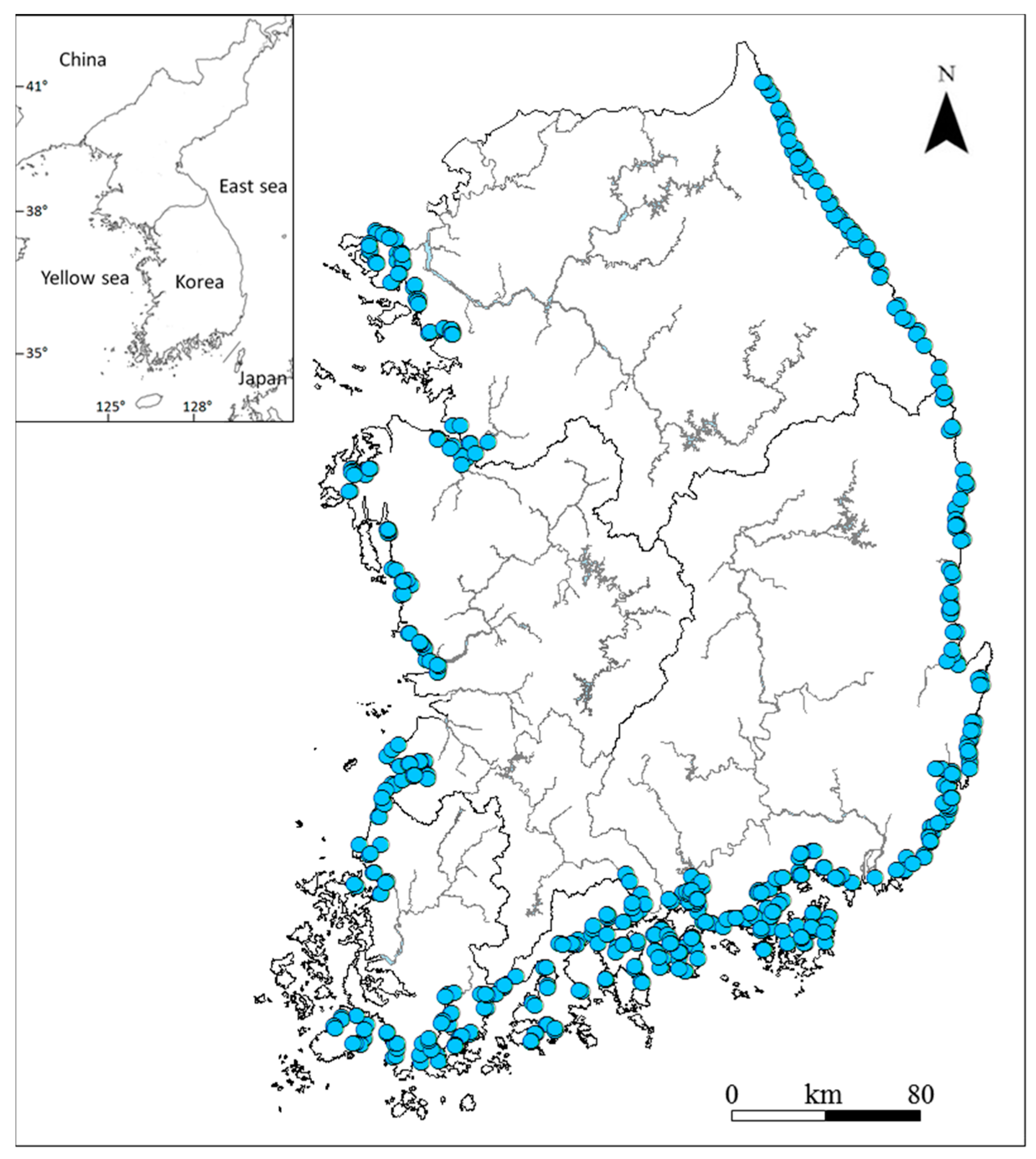
2.1. Study Area

The present study surveyed 512 estuarine zones in 317 rivers that are close to the ocean in Korea over a nine-year period (2009–2016). The selected sites are actually the total survey points designated by Ministry of Environment (MOE), Republic of Korea. Therefore, we selected all the river mouths (estuary) for the study. The surveys were conducted in May to avoid the influence of the heavy rainy season during summer. The 512 locations are not regularly and repeatedly sampled or surveyed, but only irregularly sampled in May during 2009–2016. In Korea, May has little or no impact of monsoon or rainfall against stream and estuary ecosystem. The survey sites were divided into three categories of eastern sea estuary (ESE; 135 sites), southern sea estuary (SSE; 230 sites), and western sea estuary (WSE; 147 sites) based on the nearby sea (Table 1 and Figure 1). The categorized estuaries were further divided into closed estuary (296 sites), where the estuarine circulation is cut off by estuarine dam or drainage gate, and open estuary (216 sites), where complete or partial estuarine circulation is taking place (Table 1). The sites were selected based on the 2008 Guide of MOE/National Institute of Environmental Research (NIER) [36], specifically as sites that form a boundary with the ocean and areas affected by the ocean in an upstream direction of the river.

2.2. Data Collection

2.2.1. Water Quality

Water temperature, dissolved oxygen (DO), potential hydrogen (pH), electrical conductivity (EC), salinity, and turbidity of the survey sites were measured on-site using a multi water quality checker (Horiba U-50, HORIBA Ltd., Kyoto, Japan). The water samples needed for laboratory analysis were collected in a 2-L sterilized water collection bottle from each site and transported to the laboratory while being stored on ice. Biological oxygen demand (BOD) was calculated as the difference between the DO concentration measured on-site and the DO concentration of the water sample collected on-site in a 300 mL BOD bottle and subsequently incubated in an incubator for five days at 20 °C under dark conditions, in accordance with the Winkler azide method. Concentrations of dissolved inorganic matters were measured with the ascorbic acid method using a spectrophotometer (Optizen POP, Neogen Inc., Sejong, Korea), after the cadmium reduction method was used to determine total nitrogen (TN) and persulfate decomposition for total phosphorus (TP) [37]. For chlorophyll (Chl-a) concentration and ash-free dry mass (AFDM), three or more rocks, ≥10 cm in size with a flat surface, were collected from the survey sites. A soft brush was used to clean 25 cm2 of the upper section of the collected rocks, which were placed in plastic sample bottles using water from the site. The collected samples were kept under cold and dark conditions and transported to the laboratory for measurement by standard methods [37].

2.2.2. Epilithic Diatom Community

The epilithic diatom samples that were scrubbed off with a soft brush from the upper part of the substrate collected from the survey sites were transported to the laboratory after fixing in Lugol’s solution, after which, they were washed using the permanganate method [38] and permanent samples were prepared using an encapsulant. Epilithic diatom samples were observed using an optical microscope (Nikon E600, Nikon, Tokyo, Japan) under 400× to 1000× magnification. The relative abundance of species present for the analysis of epilithic diatom communities was set to the number of diatom frustules being ≥500 under arbitrarily set microscopic field of view. Species were identified using the methods of Krammer and Lange–Bertalot [39,40] and classified according to the Simonsen’s classification system [41]. To determine the characteristics of epilithic diatom communities, the dominant species, dominance index [42], diversity index [43], richness index [44], and evenness index [45] of each survey site were derived.

2.3. Data Analysis

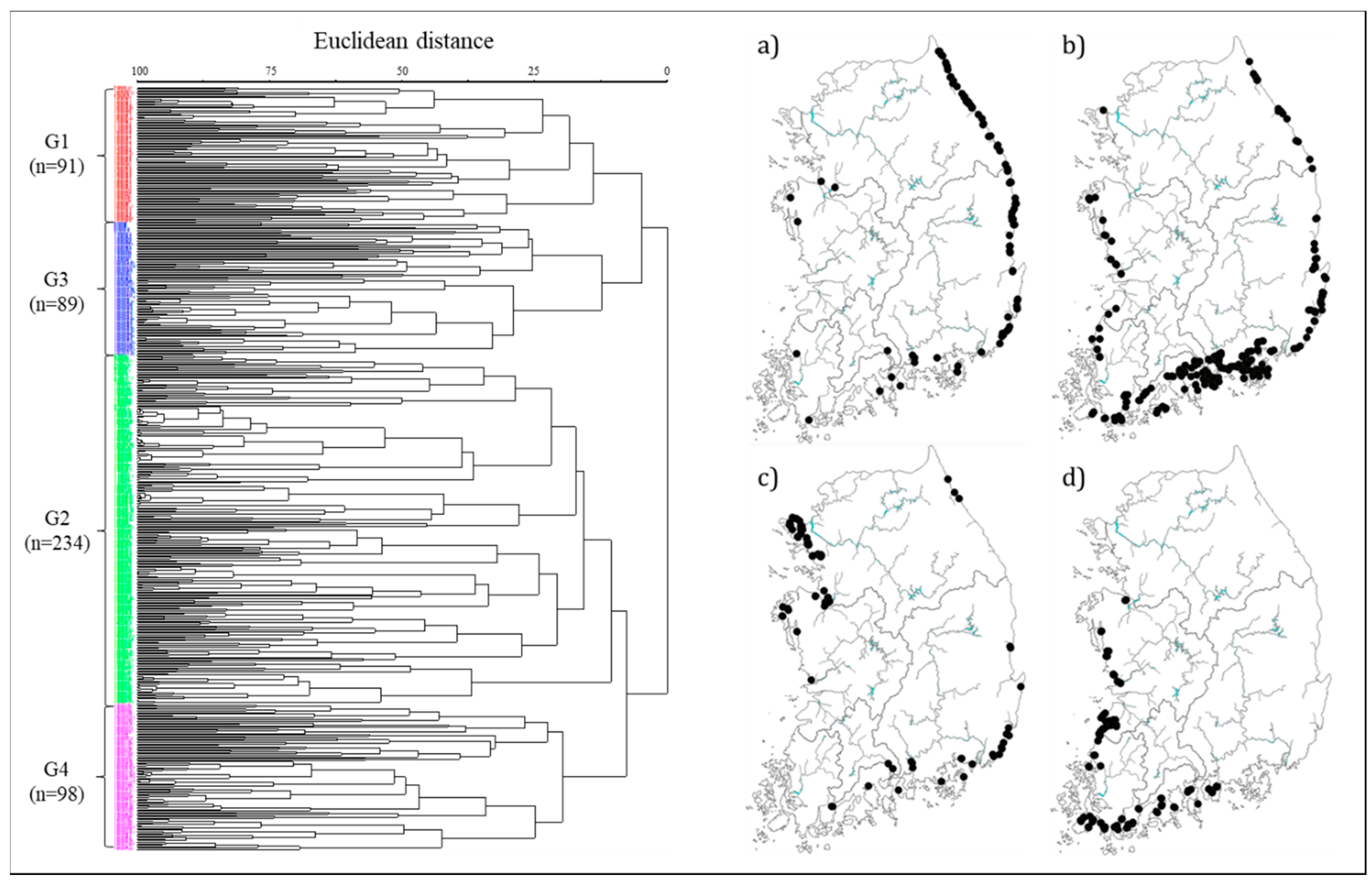
2.3.1. Cluster Analysis

To characterize the distribution of epilithic diatom communities present in estuarine zones within Korea, a cluster analysis was performed based on the number individuals in epilithic diatom communities and number of species present. In the cluster analysis, species types were classified according to similarity between cluster composition using the Ward’s linkage method and Euclidean distance.

2.3.2. Indicator Species Analysis

Indicator species analysis (ISA) was performed to determine the indicator species and indicator value (IndVal) of each group categorized by cluster analysis. The ISA is a non-hierarchical statistical analysis method that uses the relative abundance and frequency of each species at each survey site to calculate the IndVal, upon which, the indicator species is determined. In the IndVal method [46], IndVal appears within a range of 0–100 with higher values representing higher indicative power [47]. In this study, when the IndVal was ≥25, the species with IndVal that was five times higher than that of another group (good species) was selected as the indicator species for that group [48]. The Monte Carlo test was performed to determine the significance of the indicator species analysis.

2.3.3. Random Forest

The random forest model was used to predict the presence of epilithic diatom species. The random forest model is a non-parametric method used to estimate and assess the relationship between latent predictor variables and response variables [49], using various combinations of environmental variables. The importance of environmental variables used in this model was determined using minimum description length (MDL), which is used for comparing the relative importance of environmental factors [50] with MDL values converted to a range between 0 and 100. To assess the predictive power of this model, the accuracy rate and area under curve (AUC) were derived. Accuracy was measured based on the dichotomous method of presence and non-presence, with a range of 0–1. The AUC could predict the reliability of the resulting values of the model and it typically has a range of 0.5–1, but values below this range may also appear.

2.4. Biological Integrity Assessment

Various epilithic diatom indices were derived and used for the biological integrity assessment of each survey site. The trophic diatom index (TDI) was used to assess the nutritional status of rivers by calculating the IndVal according to relative density, pollution sensitivity, and level of diatoms present in each site. This approach, together with diatom assemblage index of organic water pollution (DAIpo), has been utilized for a relatively long time [23]. As the nutrient concentrations increases, the value of this index increases, whereas when pollution levels increase, the value decreases. The present study used a modified version of TDI suited for Korea [51]. Meanwhile, DAIpo was used to calculate IndVal according to organic indicators (sensitive species and tolerant species) of species present in the survey sites [21], where an increase in level of pollution results in decrease in the value of this index. The Achnanthes/Achnanthes + Navicula (AAN) index is the proportion (%) of Achnanthes among total sum of Achnanthes (saproxenous species representing clear water areas) and Navicula (eutrophic species that prefer highly polluted water areas) [52]. An increase in the level of pollution results in a decrease in the value of this index. The motile diatoms (MD) index is a value that indicates the proportion (%) of motile diatoms in heavily polluted water areas among the total amount of diatoms present in each survey site [53]. An increase in the concentration of organic matters results in an increase in the value of this index. The classification of motile diatoms in this study followed the method by Hill et al. [54]. Lastly, the number of Gomphonema species (NGO) index is a value that indicates the percentage (%) of species that are member of the Gomphonema genus among all diatom species present in each survey site [52]. An increase in concentration of organic matters results in a decrease in the value of this index.
To compare the differences in community characteristics (total number of species and biomass), community indices, and environmental factors between the groups, Tukey’s post hoc test was performed for Analysis of Variance (ANOVA) nonparametric multiple comparisons. Moreover, Pearson’s correlation analysis was employed to analyze the relationships between indicator species and environmental factors for each group.
For cluster, indicator species, and Canonical Correspondence Analyses (CCA), the PC-Ord program (ver. 4.25. MjM Software, Gleneden Beach, OR, USA) was used. The random forest model was run by the CORElearn package in R statistic program (http://cran.r-project.org). ANOVA was performed using SPSS software (ver. 21. IBM, New York, NY, USA).
For epilithic diatom community data, species that appeared in less than 5% of all survey sites (25 sites) were identified as rare taxa and excluded from the statistical analysis. Moreover, to reduce variations among individuals, data were converted to the natural log (ln) and a value of 1 was added to each variable to prevent the ln value from becoming 0.

3. Results

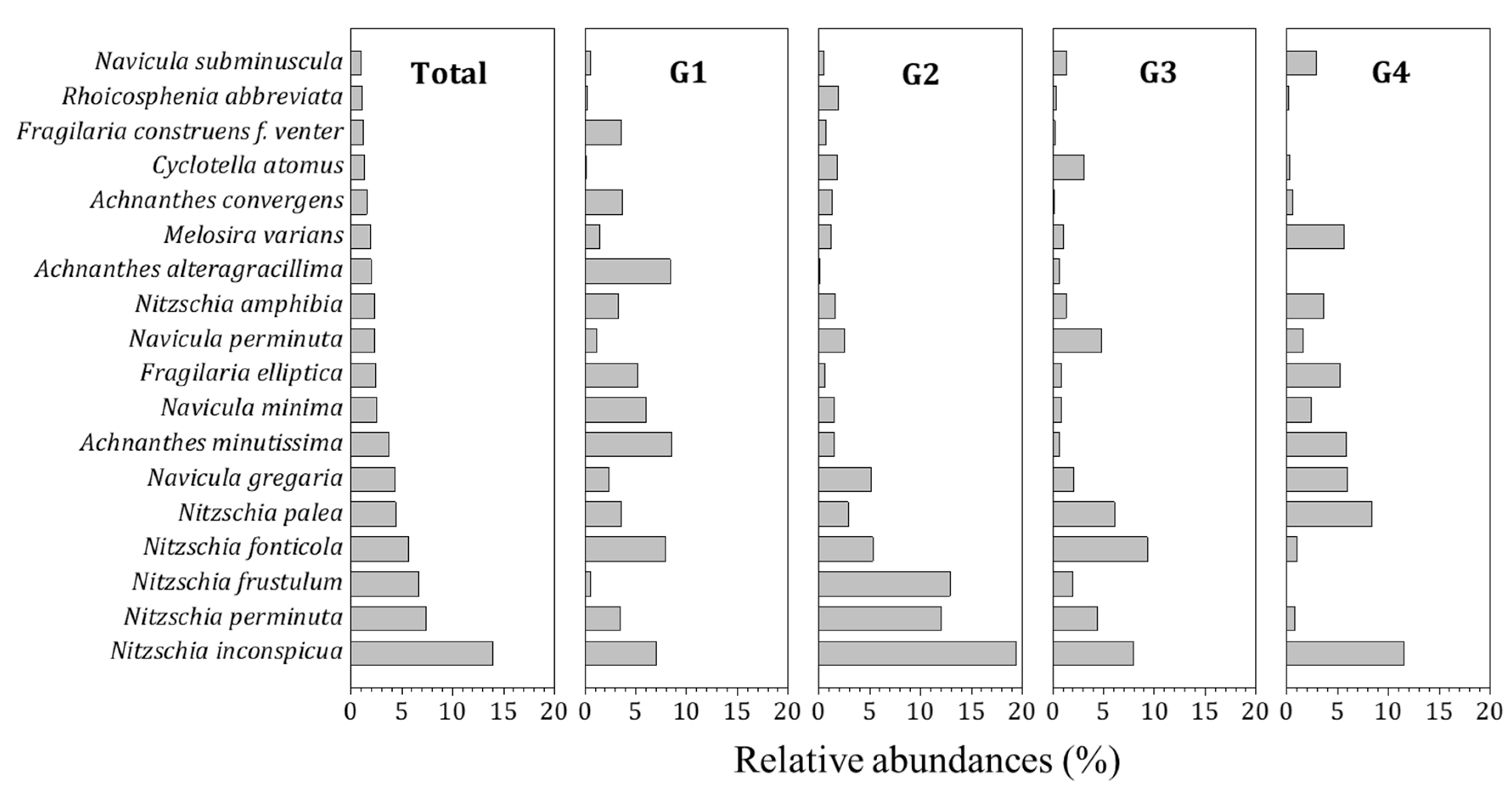
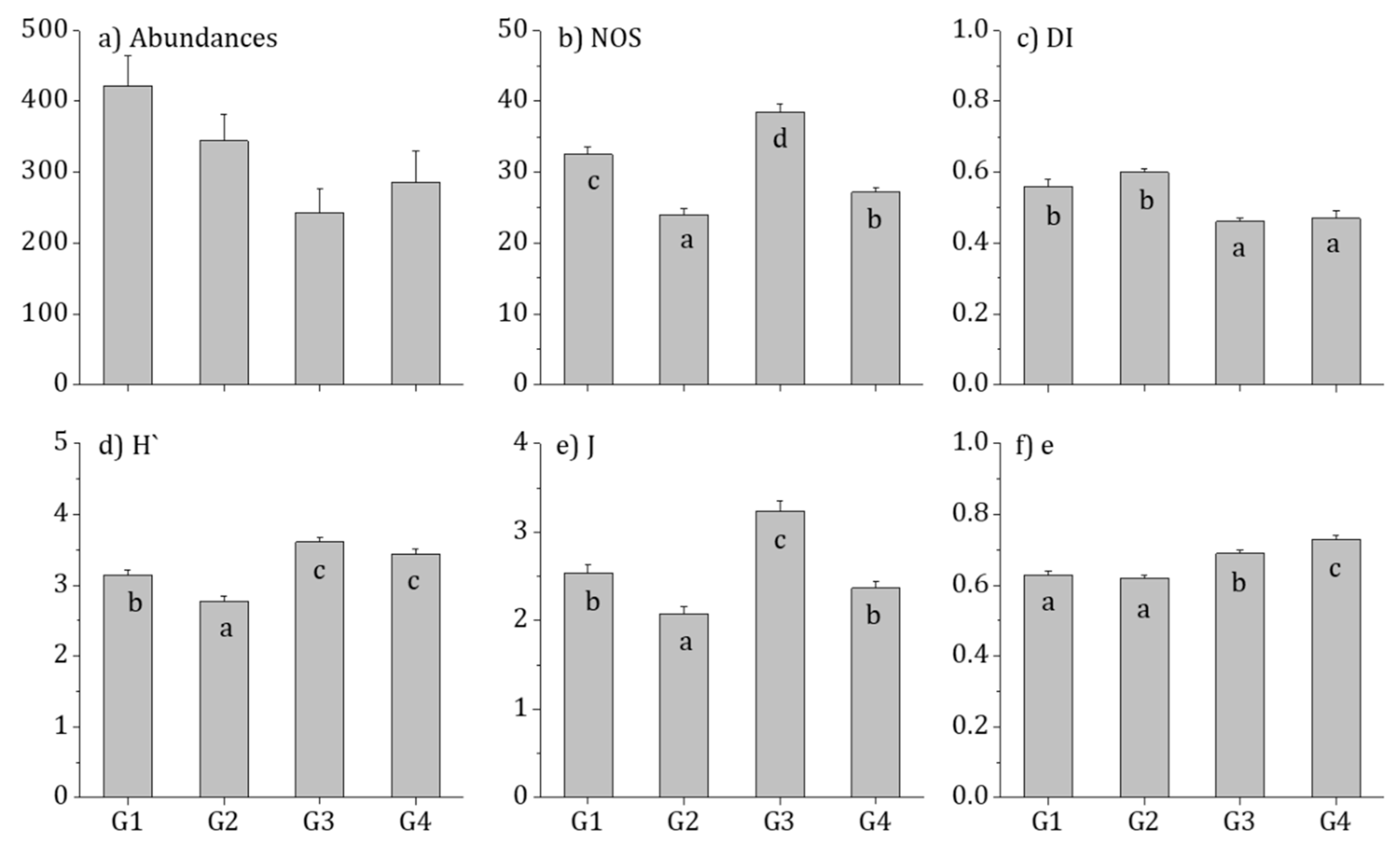
3.1. Diatom Distribution and Community Characteristics

A total of 566 taxa of epilithic diatoms were present in 512 survey sites. The dominant species was Nitzschia inconspicua (13.9%), while the subdominant species was Nitzschia perminuta (7.4%). The total number of epilithic diatom species present was highest in the southern sea with 457 species, followed in order by the eastern sea (354 species) and the western sea (346 species). Nitzschia inconspicua was the dominant species in all of the sea areas, with the highest percentage of 18.9% found in the southern sea area (Table 2).
In the cluster analysis, using the current level of presence (cell density) of a total of 139 species after excluding epilithic diatoms that were present in <5% (<25 sites) of all survey sites, the species were grouped into four groups at a 25% level: Group 1 (G1: 91 sites), Group 2 (G2: 234 sites), Group 3 (G3: 89 sites), and Group 4 (G4: 98 sites) (Figure 2). G1, comprising mostly of sites located in eastern sea region, and G2, comprising sites in the southeastern coast of the Korean Peninsula, showed relatively high percentages of open estuaries with 96% and 71%, respectively. On the other hand, G3 and G4, mostly encompassing sites located in the western sea region, displayed high percentages of closed estuaries with 61% and 93%, respectively.
With respect to the dominant epilithic diatom species in each group, Achnanthes minutissima (8.5%) and A. alteragracillima (8.4%) were the dominant species in G1, but they showed very low percentages in other groups. On the other hand, Nitzschia inconspicua, which was the dominant species for all survey sites, displayed high relative frequencies in G2 (7.9%), G3 (19.4%), and G4 (11.5%), appearing as the dominant or subdominant species (Figure 3).
With respect to biological indices in each group, G3 had the highest number of species present, while G1 and G2 exhibited higher community indices and dominance indices than G3 and G4. Moreover, G3 and G4 had significantly higher diversity indices, G3 had the highest richness index, and G4 had the highest evenness index (p < 0.01; Figure 4).
In the indicator species analysis of each group targeting 139 taxa of epilithic diatoms with frequency ≥ 5% in all survey sites, there were 16 taxa with IndVal ≥ 25%, which were considered good indicators with values more than five times higher than other groups: G1 (5 species), G3 (8 species), and G4 (3 species). Meanwhile, no indicator species appeared in G2. The species with the highest IndVal (46%) was Stephanodiscus invisitatus, which was the indicator species of G3, but all other indicator species presented IndVal ≤ 40% (Table 3).

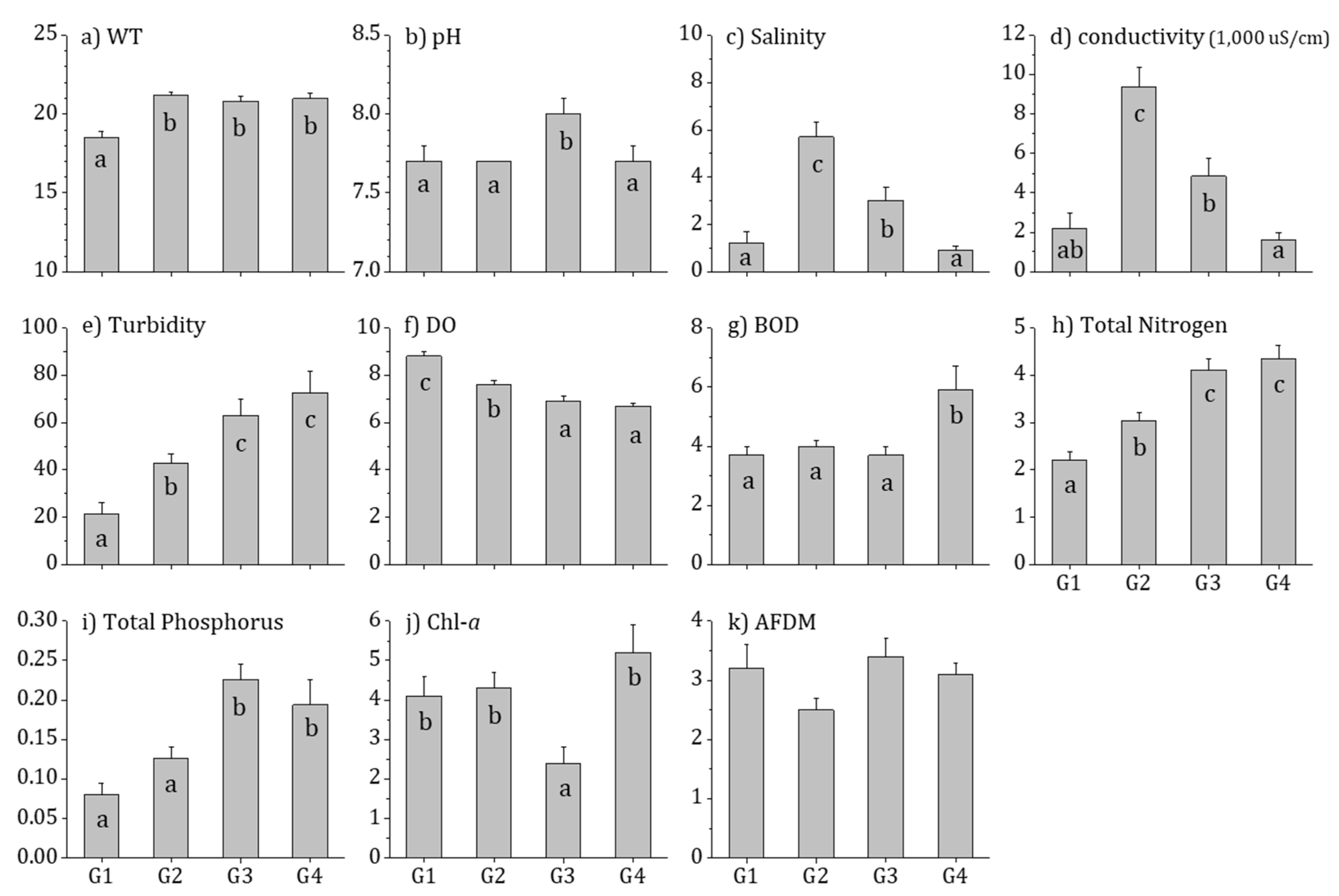
3.2. Physiochemical Water Quality

In the comparison of the physicochemical environment between the four groups (communities) categorized by distribution of epilithic diatoms using ANOVA, the factors that demonstrated significant differences were as follows (Figure 5): water temperature was lowest (18.5 °C) in G1 with highest percentage of ESE; pH (8.0) was highest in G3; and salinity (5.7 ppt) and EC (9396.8 μS/cm) were highest in G2 with highest percentage of ESE, SSE, and open estuaries (p < 0.01). Moreover, turbidity, TN, and TP were significantly higher in G3 and G4 than G1 and G2, while DO was highest in G1 and BOD was highest in G4 (p < 0.01). Consequently, the physicochemical environment of estuaries in the Korean Peninsula were classified similarly to the distribution characteristics of epilithic diatoms, except for water temperature, salinity, and EC that are affected by geographical influence. Furthermore, the results showed that water quality in the East-Southeastern Sea was better than that of the West-Southwestern Sea.

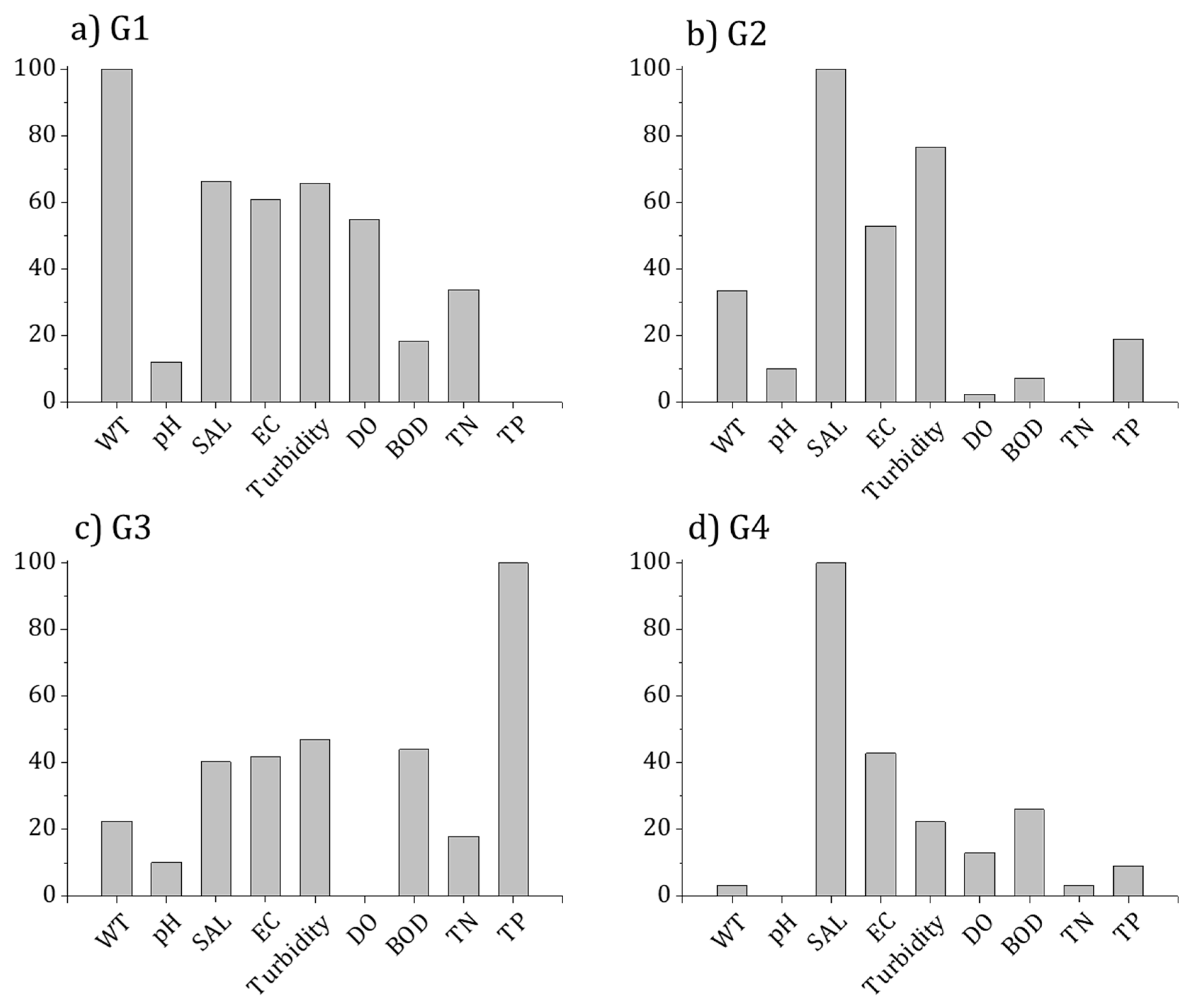
3.3. Relationship between Diatom Distribution and the Environment

In the correlation analysis between the indicator species and environmental factors of each group, most group indicator species displayed high correlations with turbidity, regardless of the groups, negative correlations with the indicator species of G1, and positive correlations with the indicator species of G3 and G4 (Table 4). In G1, Cymbella silesiaca, the species with highest IndVal in this group, showed a negative correlation with water temperature, pH, salinity, EC, turbidity, BOD, TN, TP, and AFDM, and a positive correlation with DO. In G3, Stephanodiscus invisitatus, the species with highest IndVal in this group, exhibited a positive correlation with pH, turbidity, TN, TP, and AFDM. In G4, the indicator species Bacillaria paradoxa correlated positively with turbidity, BOD, and AFDM. These results demonstrate contradicting correlations between the indicator species of G1 and the indicator species of G3 and G4.
The environmental factors that impact the presence of species in epilithic diatom communities were assessed using a random forest model. The results varied depending on the species, with accuracy ranging from 0.82 to 0.98 and the AUC displaying a range of 0.94 to 1.00 (Table 5). Among 139 taxa, the species that exhibited the highest predictive power was Navicula atomus var. permitis (accuracy: 0.98, AUC: 1.00), whereas the species with the lowest accuracy were Gomphonema lagenula, Navicula gregaria, and Nitzschia dissipata, and the species that displayed the lowest AUC value was Achnanthes convergens. To assess the contribution of environmental factors that impact the presence of epilithic diatoms, a sensitivity analysis was performed using MDL of random forest (RF). The most important factors that impacted the presence of epilithic diatoms were found to be EC (41 species, 29.5%) and salinity (36 species, 25.9%). These factors explained the presence of 55% of the species in epilithic diatom communities in estuaries. The results also showed that turbidity (13 species, 9.4%) and TN (13 species, 9.4%) were relatively important for the appearance of species in epilithic diatom communities (Table 4). Other important factors included EC for Cymbella silesiaca (indicator species with the highest IndVal in G1), pH for Stephanodiscus invisitatus (indicator species in G3), and BOD for Bacillaria paradoxa (indicator species in G4) (Table 4). Meanwhile, the main factor that determined the presence of epilithic diatoms in each group was water temperature for G1, salinity for G2 and G4, and TP for G3 (Figure 6).

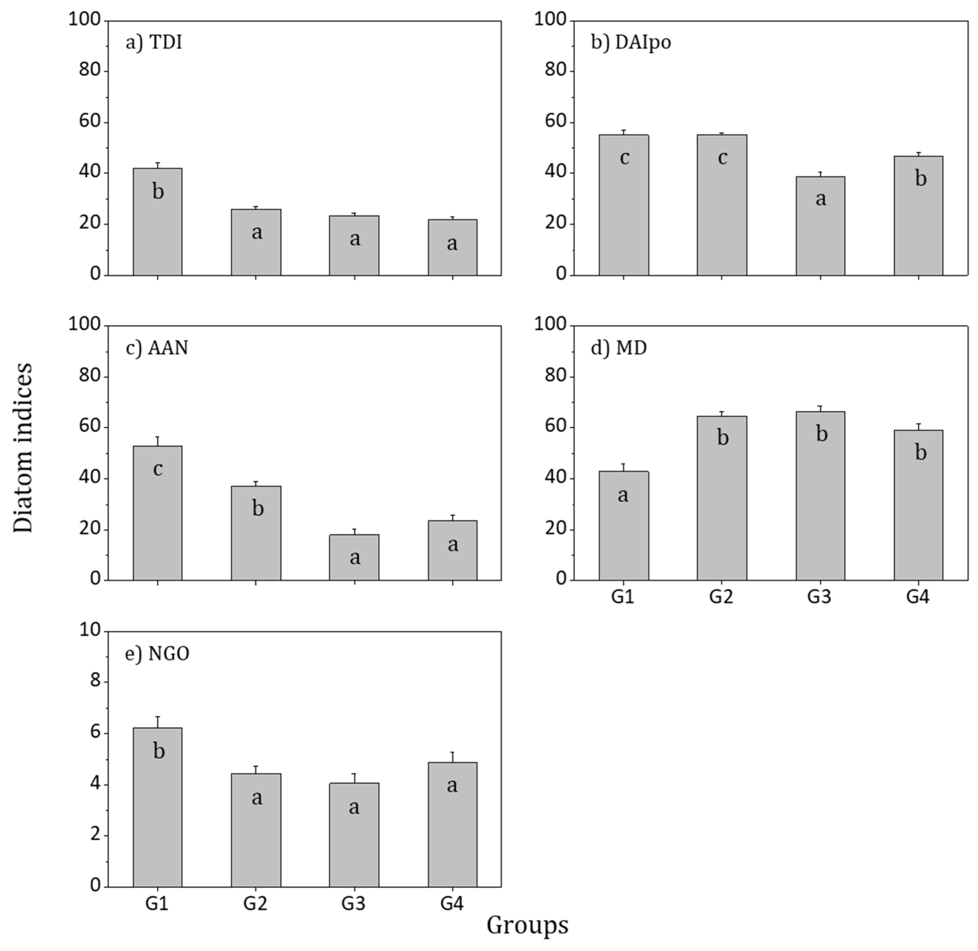
3.4. Biological Integrity and Water Quality Assessment

When comparing the four groups by ANOVA using epilithic diatom indices for the assessment of biological integrity of estuaries in the Korean Peninsula, all items demonstrated significant differences (Figure 7). TDI, DAIpo, AAN, and NGO, which are items that decrease in value when the level of pollution increases, tended to be highest in G1 and lowest in G3. MD, which increases in value when the level of pollution increases, was lowest in G1 and highest in G3. Thus, the biological integrity was assessed to be high in G1, which exhibited low nutrient levels similar to water quality characteristics, while the integrity in G3 was determined to be low, with a relatively high level of nutrients.

4. Discussion

The present study analyzed the relationships between environmental factors and the distribution of diatom communities in estuaries in the Korean Peninsula. During the study period, 566 taxa of epilithic diatoms were identified in 512 sites. These results determined a higher number of taxa than the 327 taxa found in 161 sites between 2012 and 2014 in a previous study [31], which appears to be the result of the present study having more survey sites than previous studies. With respect to dominant species, the Nitzschia genus appeared in over 38% of estuaries in the Korean Peninsula. Moreover, the dominant species in the group that was directly affected by the ocean in the Ebro estuary of Spain included Nitzschia frustulum and Nitzschia inconspicua [55]. Meanwhile, the major epilithic diatoms present in estuaries in the Korean Peninsula (Nitzschia, Navicula, Achnanthes, and Fragilaria genera) have also been widely recorded in estuaries throughout the world, including Hungary, Sweden [56], the United States [57], Argentina, Uruguay [58], and the United Kingdom [59].
Based on the similarities of epilithic diatom communities in estuaries in the Korean Peninsula, a cluster analysis was performed to categorize four groups. G1 comprised the eastern sea region that included mostly the eastern area of Han River and parts of Nakdong River. G2 spread widely across the eastern and southern sea regions that included the eastern part of Han River, Nakdong River, and Seomjin River. According to Rho and Lee [4], land cover types in estuaries located in the eastern regions of Han River and Nakdong River showed a high percentage for forest (60%) and a low percentage for farmland (≤20%).
G1, located in eastern sea region, had low nutrient concentrations and significantly low levels of salinity and turbidity. This is consistent with previous studies where forest land use was reported to have a negative correlation with nutrient levels [60,61]. Furthermore, because there is a continuation of the ridgeline with rapidly descending altitude that extends from the Tae Baek Mountains to the East Sea, small rivers flowing into the East Sea have steep downward slopes and short extended waterways [62]. Tidal variations in this coast are minimal, and, thus, the tidal effects are usually very weak [63]. Accordingly, estuaries located on the eastern coast display lower salinity than those located on the western or southern coasts.
G3, located in the western sea region, included mostly the eastern section of Han River and parts of Geum River. G4, located in the western and southern sea regions, comprised mostly of the Geum and Yeongsan Rivers. The Geum River and Yeongsan River regions have proportions of farmland of ≥ 35%, which are much higher than the average of 28.8% for Korea. This is because of an increase in farming area from large-scale land reclamation by drainage and land clearing projects concentrated in these regions [4].
G3 and G4, located in western and southwestern estuaries, demonstrated significantly high levels of nutrients and turbidity. A previous study reported that a high percentage of farmland is highly correlated with total suspended solids (TSS) [64,65]. Moreover, when farmland is the type of land use, strong positive correlations with nutrients such as TN and TP are found [60], and as turbidity increases, DO concentration is known to decrease [66,67]. Furthermore, salinity and EC appeared at significantly high levels in G2, which appears to be the result of seawater flowing deeply into the estuaries due to the high percentage of open estuaries in the southern sea region.
Achnanthes alteragracillima, the subdominant species in G1, was almost not present in other groups, and this species is a saproxenous species that is present in relatively clean water. Nitzschia inconspicua, the dominant species in G2, G3, and G4, also appeared as the dominant species in 30 estuaries in 2012 [30].
Cymbella silesiaca, Fragilaria rumpens var. fragilarioides, and Reimeria sinuata, the indicator species of G1, correlated positively with DO and negatively with salinity, EC, turbidity, BOD, TN, and TP (Table 4). These species are typical saproxenous species [68], which are known to grow in oligotrophic and mesotrophic waters [69]. Stephanodiscus invisitatus, Cyclotella atomus, Stephanodiscus hantzschii, Navicula veneta, and Navicula accomoda, the indicator species in G3, displayed positive correlations with salinity, turbidity, TN, and TP and a negative correlation with DO (Table 4). These species grow mostly by floating in freshwater with high EC or are present in brackish water zones in rivers. They are known to be tolerant to organic pollutants [70,71]. The indicator species in G4, Bacillaria paradoxa, Navicula capitate, and Nitzschia calida, showed positive correlations with turbidity and BOD (Table 4). These species grow in brackish water zones or eutrophic waters with high EC, and they are known to have broad range of tolerance to pollutants.
Environmental factors that influence species presence or emergence in epilithic diatom communities were predicted using a random forest model (Table 5). The results showed that the most important factors were EC (41 species, 29.5%) and salinity (36 species, 25.9%). These factors explained the existence of 55% of the species in epilithic diatom communities in estuaries. Turbidity (13 species, 9.4%) and TN (13 species, 9.4%) also appeared as being relatively important for species presence in epilithic diatom communities. EC is known to be an important factor for determining the composition of epilithic diatom community [72,73].
In a preliminary study on diatom distribution associated with salinity, the salinity gradient was mostly the result of changes in the concentration of a single salt, sodium chloride (NaCl) [74,75,76]. As a result, it was difficult to differentiate the effect of a specific ion and the overall effect of osmotic pressure. Experimental results showed that medium osmotic pressure was an important factor in limiting the growth of freshwater diatoms [77] and affected nutrient intake [78]. Therefore, total ion strength and EC can explain the significant changes between diatom communities [72]. Amino acid, ammonium, and nitrate, which are a types of nitrogen compounds, are nutrients preferred by marine benthic diatoms [79]; however, because the present study only measured TN, it is necessary to conduct further experiments to measure a greater variety of nitrogen compounds. Therefore, if more detailed water quality (various nitrogen compounds and ions) measurements were conducted in the future, then more definitive evidence for distribution of epilithic diatoms might be available.
As a result of biological integrity assessment using epilithic diatom indices, the TDI could be divided into grades from A for very good to E for very poor, in accordance with the grading system given in the Biomonitoring Survey and Assessment Manual [51]. The TDI grade for estuaries was C (average) in G1, which had the highest IndVal of 42, while all other groups had a grade of D (poor). Compared to river water quality standards in Korea, G1 was assessed as having very good DO, somewhat good TP, and average BOD, with a TDI grade slightly lower than the water quality grade. Moreover, DAIpo, AAN, and NGO also showed low values below 50, relative to 100. This is because most of the epilithic diatom indices used in the present study were developed for freshwater systems, and thus, species that are ecologically important in estuaries were not included in the indices [80]. Moreover, some species that are included in the biological indices may not respond the same to environmental situations in estuaries and freshwater. For example, N. frustulum, which appeared as a major species with a high percentage of 6.7%, is very abundant in freshwater due to the high level of organic matters [81], high concentrations of inorganic nutrients [82], and high EC [82,83]. However, they may be present in high levels in estuaries without showing any reduction in health [80]. Nanivula perminuta, another major species, exhibited different concentrations in ammonium and nitrate that showed a peak growth rate according to salt concentrations [84]. Therefore, to establish the biological impact assessment system using epilithic diatoms in water areas with severe fluctuation, such as estuaries, it is necessary to adjust the index values according to the nutritional status of the estuary instead of using freshwater indices as they are. Additional studies are also required to further understand the role of epilithic diatom communities.

5. Conclusions

Between 2009 and 2016 during May, we assessed the feasibility of applying diatom indices previously studied to assess the biological integrity of estuaries, while also predicting the importance of environmental factors and species appearance of epilithic diatoms in the southern part of the Korean Peninsula.
1. In total, 564 taxa of diatoms were found and the dominant species were identified as Nitzschia inconspicua and N. perminuta.
2. According to the species appearance and their abundances of diatoms, estuaries in the Korean Peninsula were geographically categorized into four groups. G1 showed high water temperature and DO levels, while nutrient levels were significantly low. G3 and G4 showed significantly high turbidity and nutrient levels.
3. A random forest model indicated that the major factors predicting diatom appearance in estuary are electric conductivity, salinity, turbidity, and total nitrogen.
4. The biological integrity of the estuary of Korean peninsula using “stream diatom indices” is very low through the sampling sites; however, a de novo diatom index should be developed to assess different or specialized ecosystem of estuary.

Author Contributions

H.-K.K., I.-H.C., and E.-A.H. collected the diatom samples. B.-H.K. contributed to the writing of the manuscript and participated in discussions regarding the appropriate groups for analysis, and Y.-J.K. helped in manuscript revision. All authors approved the final manuscript.

Funding

This study was supported by the Ministry of Environment and the National Institute of Environmental Research (Korea).

Acknowledgments

The authors would like to thank all of the survey members involved in the project for their help in sampling and analyses. The authors also thank the reviewers for their help in improving the scientific quality of the manuscript. We would like to thank Editage (www.editage.co.kr) for English language editing.

Conflicts of Interest

The authors declare no conflict of interest.

References

  1. Westen, C.J.; Scheele, R.J. Characteristics of Estuaries. In Planning Estuaries; Springer: New York, NY, USA, 1996; pp. 9–60. [Google Scholar]
  2. Flemer, D.A.; Champ, M.A. What is the future fate of estuaries given nutrient over-enrichment, freshwater diversion and low flows? Mar. Pollut. Bull. 2006, 52, 247–258. [Google Scholar] [CrossRef] [PubMed]
  3. Silva, M.A.M.; Eça, G.F.; Felix, D.F.; Santos, D.F.; Guimarães, A.G.; Lima, M.C.; de Souza, M.F.L. Dissolved inorganic nutrients and chlorophyll a in an estuary receiving sewage treatment plant effluents: Cachoeira River estuary (NE Brazil). Environ. Monit. Assess. 2013, 185, 5387–5399. [Google Scholar] [CrossRef] [PubMed]
  4. Rho, P.H.; Lee, C.H. Spatial Distribution and Temporal Variation of Estuarine Wetlands by Estuary Type. J. Korean Geogr. Soc. 2014, 49, 321–338. [Google Scholar]
  5. Ohrel, R.L.; Register, K.M. (Eds.) Voluntary Estuary Monitoring Manual; Environmental Protection Agency: Washington, DC, USA, 2006. Available online: https://www.epa.gov/sites/production/files/2015-09/documents/2007_04_09_estuaries_monitoruments_manual.pdf (accessed on 26 July 2019).
  6. Lee, K.H.; Rho, B.H.; Cho, H.J.; Lee, C.H. Estuary Classification Based on the Characteristics of Geomorphological Features, Natural Habitat Distributions and Land Uses. J. Korean Soc. Oceanogr. 2011, 16, 53–69. [Google Scholar] [Green Version]
  7. Cloern, J.E.; Powell, T.M.; Huzzey, L.M. Spatial and temporal variability in South San-Francisco Bay (USA). Temporal changes in salinity, suspended sediments, and phytoplankton biomass and productivity over tidal time scales. Estuar. Coast. Shelf Sci. 1989, 28, 599–613. [Google Scholar] [CrossRef]
  8. Webster, I.T.; Parslow, J.S.; Smith, S.V. Implications of spatial and temporal variation for biogeochemical budgets of estuaries. Estuarine 2000, 23, 341–350. [Google Scholar] [CrossRef]
  9. Rovira, L.; Trobajo, R.; Ibáñez, C. Periphytic diatom community in a Mediterranean salt wedge estuary: The Ebro Estuary (NE Iberian Peninsula). Acta Bot. Croat. 2009, 68, 285–300. [Google Scholar]
  10. Smol, J.P.; Stoermer, E.F. The Diatoms: Applications for the Environmental and Earth Sciences, 2nd ed.; University Press: Cambridge, UK, 2010. [Google Scholar]
  11. Meleder, V.; Rincé, Y.; Barillé, L.; Gaudin, P.; Rosa, P. Spatiotemporal changes in microphytobenthos assemblages in a macrotidal flat (Bourgneuf Bay, France). J. Phycol. 2007, 43, 1177–1190. [Google Scholar] [CrossRef]
  12. Biggs, B.J.; Goring, D.G.; Nikora, V.I. Subsidy and stress responses of stream periphyton to gradients in water velocity as a function of community growth form. J. Phycol. 1998, 34, 598–607. [Google Scholar] [CrossRef]
  13. Ewe, S.M.L.; Gaiser, E.E.; Childers, D.L.; Rivera-Monroy, V.H.; Iwaniec, D.; Fourquerean, J.; Twilley, R.R. Spatial and temporal patterns of aboveground net primary productivity (ANPP) in the Florida Coastal Everglades LTER (2001–2004). Hydrobiologia 2006, 569, 459–474. [Google Scholar] [CrossRef]
  14. Evelyn, G. Periphyton as an indicator of restoration in the Florida Everglades. J. Ecol. Indic. 2009, 9, 37–45. [Google Scholar]
  15. Lamberti, G.A. Grazing experiments in artificial streams. J. N. Am. Benthol. Soc. 1993, 12, 337–343. [Google Scholar]
  16. Leland, H.V.; Porter, S.D. Distribution of benthic algae in the upper Illinois River basin in relation to geology and land use. Freshw. Biol. 2000, 44, 279–301. [Google Scholar] [CrossRef]
  17. McCormick, P.V.; Stevenson, R.J. Periphyton as a tool for ecological assessment and management in the Florida Everglades. J. Phycol. 1998, 34, 726–733. [Google Scholar] [CrossRef]
  18. Maarten, D.J.; Vijverb, B.V.; Blusta, R.; Bervoets, L. Responses of aquatic organisms to metal pollution in a lowland river in Flanders: A comparison of diatoms and macroinvertebrates. Sci. Total Environ. 2008, 407, 615–629. [Google Scholar]
  19. Kim, N.; Thomas, I.; Murphy, P. Assessment of eutrophication and phytoplankton community impairment in the Buffalo River area of concern. J. Great Lakes Res. 2009, 35, 83–93. [Google Scholar]
  20. Maria, J.F.; Almeida, S.F.P.; Craveiro, S.C.; Calado, A.J. A comparison between biotic indices and predictive models in stream water quality assessment based on benthic diatom communities. J. Ecol. Indic. 2009, 9, 497–507. [Google Scholar] [Green Version]
  21. Watanabe, T.; Asai, K.; Houki, A. Numerical estimation of organic pollution of flowing water by using the epilithic diatom assemblage—Diatom Assemblage Index (DAIpo). Sci. Total Environ. 1986, 55, 209–218. [Google Scholar] [CrossRef]
  22. Coste, M.; Boutry, S.; Tison-Rosebery, J.; Delmas, F. Improvements of the Biological Diatom Index (BDI): Description and efficiency of the new version (BDI-2006). J. Ecol. Indic. 2009, 9, 621–650. [Google Scholar] [CrossRef]
  23. Kelly, M.G.; Adam, C.; Graves, A.C.; Jamieson, J.; Krokowski, J.; Lycett, E.B.; Murray-Bligh, J.; Pritchard, S.; Wilkins, C. The Trophic Diatom Index: A User’s Manual, R&D Technical Report E2/TR2, Revised ed.; Environment Agency: Bristol, UK, 2001.
  24. Cemagref. Etude des Methodes Biologiques Quantitative D’Appreciation de la Qualite des Eaux; Rapport Q.E. Lyon- A.F. Bassin; Rhône-Méditerranée-Corse: Lyon, France, 1982; p. 218. [Google Scholar]
  25. Stevenson, R.J.; Smol, J.P. Use of Algae in Environmental Assessments. In Freshwater Algae in North America: Classification and Ecology; Academic Press: New York, NY, USA, 2003. [Google Scholar]
  26. The Ministry of Environment/National Institute of Environmental Research (MOE/NIER). Nationwide Aquatic Ecological Monitoring Program; MOE/NIER: Incheon, Korea, 2008–2018.
  27. Bogaczewicz-Adamczak, B.; Dziengo, M. Using benthic diatom communities and diatom indices to assess water pollution in the Puck Bay (southern Baltic Sea) littoral zone. Oceanol. Hydrobiol. Stud. 2003, 32, 131–157. [Google Scholar]
  28. Zgrundo, A.; Bogaczewicz-Adamczak, B. Applicability of diatom indices for monitoring water quality in coastal streams in the Gulf of Gdańsk region northern Poland. Oceanol. Hydrobiol. Stud. 2004, 33, 31–46. [Google Scholar]
  29. Della Bella, V.; Puccinelli, C.; Marcheggiani, S.; Mancini, L. Benthic diatom communities and their relationship to water chemistry in wetlands of central Italy. Annales De Limnologie. Int. J. Limnol. 2007, 43, 89–99. [Google Scholar] [CrossRef]
  30. Kim, H.K.; Kim, Y.J.; Won, D.H.; Hwang, S.J.; Hwang, S.O.; Kim, B.H. Spatial and temporal distribution of epilithic diatom communities in major harbors of Korean Peninsula. J. Korean Soc. Water Environ. 2013, 29, 598–609. [Google Scholar]
  31. Kim, H.K.; Kwon, Y.S.; Kim, Y.J.; Kim, B.H. Distribution of epilithic diatoms in estuaries of the Korean Peninsula in relation to environmental variables. Water 2015, 7, 6702–6718. [Google Scholar] [CrossRef]
  32. Yoon, K.T.; Park, H.S.; Chang, M. Implication to ecosystem assessment from distribution pattern of subtidal macrobenthic communities in Nakdong River Estuary. J. Korean Soc. Oceanogr. 2011, 16, 246–253. [Google Scholar]
  33. Kim, C.H.; Kang, E.J.; Yang, H.; Kim, K.S.; Chol, W.S. Characteristics of fish fauna collected from Near Estuary of Seomjin River and population ecology. Korean J. Environ. Biol. 2012, 30, 319–327. [Google Scholar] [CrossRef]
  34. Lee, Y.K.; Ahn, K.H. Actual vegetation and vegetation structure at the coastal sand bars in the Nakdong Estuary, South Korea. Korean J. Environ. Ecol. 2012, 26, 911–922. [Google Scholar]
  35. Shin, Y.K. An ecological study of phytoplankton community in the Geum River Estuary. Korean J. Ecol. Environ. 2013, 46, 524–540. [Google Scholar]
  36. The Ministry of Environment/National Institute of Environmental Research (MOE/NIER). Survey and Evaluation of Aquatic Ecosystem Health in Korea; MOE/NIER: Incheon, Korea, 2008.
  37. American Public Health Association (APHA). Standard Methods for the Examination of Water and Waste Water; APHA: Washington, DC, USA, 2001. [Google Scholar]
  38. Hendey, N.I. The permanganate method for cleaning freshly gathered diatoms. Microscopy 1974, 32, 423–426. [Google Scholar]
  39. Krammer, K.; Lange-Bertalot, H. Süsβwasserflora von Mitteleuropa, Band 2/1: Bacillariophyceae 1. Teil: Naviculaceae; Ettl, H., Gerloff, J., Heying, H., Mollenhauer, D., Eds.; Elsevier Book Co.: Berlin, Germany, 2007. [Google Scholar]
  40. Krammer, K.; Lange-Bertalot, H. Süsβwasserflora von Mitteleuropa, Band 2/1: Bacillariophyceae 1. Teil: Basillariaceae, Epithemiaceae, Surirellaceae; Ettl, H., Gerloff, J., Heying, H., Mollenhauer, D., Eds.; Elsevier Book Co.: Berlin, Germany, 2007. [Google Scholar]
  41. Simonsen, R. The diatom system: Ideas on phylogeny. Bacillaria 1979, 2, 9–71. [Google Scholar]
  42. McNaughton, S.J. Relationships among functional properties of Californian grassland. Nature 1967, 216, 168–169. [Google Scholar] [CrossRef]
  43. Shannon, C.E.; Weaver, W. The Mathematical Theory of Communication; University of Illinois Press: Champagne, IL, USA, 1959. [Google Scholar]
  44. Margalef, R. Information Theory in Ecology. Gen. Syst. 1958, 3, 36–71. [Google Scholar]
  45. Pielou, E.C. Ecological Diversity; Wiley: New York, NY, USA, 1975. [Google Scholar]
  46. Dufrene, M.; Legendre, P. Species assemblages and indicator species: The need for flexible asymmetrical approach. Ecol. Monogr. 1997, 67, 345–366. [Google Scholar] [CrossRef]
  47. Peterson, W.T.; Keister, J.E. Interannual variability in copepod community composition at a coastal station in the northern California Current: A multivariate approach. Deep Sea Res. Part. II Top. Stud. Oceanogr. 2003, 50, 2499–2517. [Google Scholar] [CrossRef]
  48. Keister, J.E.; Peterson, W.T. Zonal and seasonal variations in zooplankton community structure off the central Oregon coast, 1998–2000. Prog. Oceanogr. 2003, 57, 341–361. [Google Scholar] [CrossRef]
  49. Breiman, L. Random forests. Mach. Learn. 2001, 45, 5–32. [Google Scholar] [CrossRef]
  50. Robnik-Šikonja, M. Improving random forests. In Machine Learning: ECML 2004; Springer: Berlin/Heidelberg, Germany, 2004; pp. 359–370. [Google Scholar]
  51. The Ministry of Environment/National Institute of Environmental Research (MOE/NIER). Biomonitoring Survey and Assessment Manual; MOE/NIER: Incheon, Korea, 2017.
  52. Wang, Y.K.; Stevenson, R.J.; Metzmeier, L. Development and evaluation of a diatom-based Index of Biotic Integrity for the Interior Plateau Ecoregion, USA. J. N. Am. Benthol. Soc. 2005, 24, 990–1008. [Google Scholar] [CrossRef]
  53. Passy, S.I. Spatial paradigms of lotic diatom distribution: A landscape ecology perspective. J. Phycol. 2001, 37, 370–378. [Google Scholar] [CrossRef]
  54. Hill, B.H.; Herlihy, A.T.; Kaufmann, P.R.; DeCelles, S.J.; Vander Borgh, M.A. Assessment of streams of the eastern United States using a periphyton index of biotic integrity. Ecol. Indic. 2003, 2, 325–338. [Google Scholar] [CrossRef]
  55. Rovira, L.; Trobajo, R.; Leira, M.; Ibáñez, C. The effects of hydrological dynamics on benthic diatom community structure in a highly stratified estuary: The case of the Ebro Estuary (Catalonia, Spain). Estuar. Coast. Shelf Sci. 2012, 101, 1–14. [Google Scholar] [CrossRef]
  56. Kovács, C.; Kahlert, M.; Padisák, J. Benthic diatom communities along pH and TP gradients in Hungarian and Swedish streams. J. Appl. Phycol. 2006, 18, 105–117. [Google Scholar] [CrossRef]
  57. Potapova, M.G.; Charles, D.F. Benthic diatoms in USA rivers: Distributions along spatial and environmental gradients. J. Biogeogr. 2002, 29, 167–187. [Google Scholar] [CrossRef]
  58. Licursi, M.; Sierra, M.V.; Gómez, N. Diatom assemblages from a turbid coastal plain estuary: Río de la Plata (South America). J. Mar. Syst. 2006, 62, 35–45. [Google Scholar] [CrossRef]
  59. Underwood, G.; Phillips, J.; Saunders, K. Distribution of estuarine benthic diatom species along salinity and nutrient gradients. Eur. J. Phycol. 1998, 33, 173–183. [Google Scholar] [CrossRef]
  60. Tong, S.T.; Chen, W. Modeling the relationship between land use and surface water quality. J. Environ. Manag. 2002, 66, 377–393. [Google Scholar] [CrossRef]
  61. Lee, S.W.; Hwang, S.J. Investigation on the relationship between land use and water quality with spatial dimension, reservoir type and shape complexity. J. Korean Inst. Landsc. Archit. 2007, 34, 1–9. [Google Scholar]
  62. Hwang, S.I.; Yoon, S.O. Geomorphic characteristics of coastal lagoons and river basins, and sedimentary environment at river mouths along the Middle East Coast in the Korean Peninsula. J. Korean Geomorphol. Assoc. 2008, 15, 17–33. [Google Scholar]
  63. Ha, K.H. Geomorphological Characteristics and Salinity Distribution of Natural Estuaries in the East Sea (Yeongokcheon Stream, Gangneung-si and Namdea Stream, Yangyang-Gun); Seoul National University: Seoul, Korea, 2009. [Google Scholar]
  64. Allan, J.D.; Erickson, D.L.; Fay, J. The influence of catchment land use on stream integrity across multiple spatial scales. Freshw. Biol. 1997, 37, 149–161. [Google Scholar] [CrossRef] [Green Version]
  65. Johnson, L.B.; Richards, C.; Host, G.E.; Arthur, J.W. Landscape influences on water chemistry in midwestern stream ecosystems. Freshw. Biol. 1997, 37, 193–208. [Google Scholar] [CrossRef]
  66. Azim, M.E.; Milstein, A.; Wahab, M.A.; Verdegam, M.C.J. Periphyton-water quality relationships in fertilized fishponds with artificial substrates. Aquaculture 2003, 228, 169–187. [Google Scholar] [CrossRef]
  67. Park, C.G.; Kang, M.A. Impact assessment of turbidity water caused clays on algae growth. J. Eng. Geol. 2006, 16, 403–409. [Google Scholar]
  68. Watanabe, T.; Ohtsuka, T.; Tuji, A.; Houki, A. Picture Book and Ecology of the Freshwater Diatoms; Uchida-Rokakuho: Tokyo, Japan, 2005. [Google Scholar]
  69. Krammer, K.; Lange-Bertalot, H. Bacillariophyceae 4. Teil: Achnanthaceae, Kritische Erganzungen zu Navicula (Lineolate) und Gomphonema Gesammliteraturverzeichnis; Gustav Fischer Verlag: Jena, Germany, 1991. [Google Scholar]
  70. Kobayasi, H.; Mayama, S. Evaluation of river water quality by diatoms. Korean J. Phycol. 1989, 4, 121–133. [Google Scholar]
  71. Lange-Bertalot, H. Navicula sensu stricto 10 genera separated from Navicula sensu lato Frustulia. In Diatoms of Europe: Diatoms of the European Inland Waters and Comparable Habitats; Gantner Verlag: Ruggell, Germany, 2001; Volume 2, p. 526. [Google Scholar]
  72. Potapova, M.; Charles, D.F. Distribution of benthic diatoms in US rivers in relation to conductivity and ionic composition. Freshw. Biol. 2003, 48, 1311–1328. [Google Scholar] [CrossRef]
  73. Soininen, J.; Paavola, R.; Muotka, T. Benthic diatom communities in boreal streams: Community structure in relation to environmental and spatial gradients. Ecography 2004, 27, 330–342. [Google Scholar] [CrossRef]
  74. Kolbe, R.W. Zur Okologie, Morphologie und Systematik der Brackwasser-Diatomeen. Pflanzenforschung 1927, 7, 1–146. [Google Scholar]
  75. Kolbe, R.W. Grundlinien einer allgemeinen Ökologie der Diatomeen. Ergeb. Biol. 1932, 8, 221–348. [Google Scholar]
  76. Hustedt, F. Die Diatomeenflora des Fluss-systems der Weser in Gebiet der Hansestadt Bremen. Abh. Nat. Ver. Brem. 1957, 34, 181–440. [Google Scholar]
  77. Cleave, M.L.; Porcella, D.B.; Adams, V.D. The application of batch bioassay techniques to the study of salinity toxicity to freshwater phytoplankton. Water Res. 1981, 15, 573–584. [Google Scholar] [CrossRef]
  78. Tuchman, M.L.; Theriot, E.; Stoermer, E.F. Effects of low-level salinity concentrations on the growth of Cyclotella meneghiniana Kütz (Bacillariophyta). Arch. Protistenkd. 1984, 128, 319–326. [Google Scholar] [CrossRef]
  79. Admiraal, W.; Riaux-Gobin, C.; Laane, R.W. Interactions of ammonium, nitrate, and D-and L-amino acids in the nitrogen assimilation of two species of estuarine benthic diatoms. Mar. Ecol. Prog. Ser. 1987, 40, 267–273. [Google Scholar] [CrossRef]
  80. Rovira, L.; Trobajo, R.; Ibáñez, C. The use of diatom assemblages as ecological indicators in highly stratified estuaries and evaluation of existing diatom indices. Mar. Pollut. Bull. 2012, 64, 500–511. [Google Scholar] [CrossRef] [PubMed]
  81. Leira, M.; Sabater, S. Diatom assemblages distribution in Catalan Rivers, NE Spain, in relation to chemical and physiographical factors. Water Res. 2005, 39, 73–82. [Google Scholar] [CrossRef] [PubMed]
  82. Van Dam, H.; Mertens, A.; Sinkeldam, J. A coded checklist and ecological indicator values of freshwater diatoms from The Netherlands. Neth. J. Aquat. Ecol. 1994, 28, 117–133. [Google Scholar]
  83. Rimet, F. Benthic diatom assemblages and their correspondence with ecoregional classifications: Case study of rivers in north-eastern France. Hydrobiologia 2009, 636, 137–151. [Google Scholar] [CrossRef]
  84. Underwood, G.J.; Provot, L. Determining the environmental preferences of four estuarine epipelic diatom taxa: Growth across a range of salinity, nitrate and ammonium conditions. Eur. J. Phycol. 2000, 35, 173–182. [Google Scholar] [CrossRef]
Figure 1. A map showing the 512 sampling stations for the water and diatom sampling in Korean estuaries between 2009 and 2016.
Ijerph 16 02681 g001
Figure 2. (Left) Dendrogram illustrating the sites affinity by cluster analysis with diatom abundance and appearance. Each color in figures presents four groups: G1 (red), G2 (green), G3 (blue), and G4 (pink). (Right) Geographical distribution patterns of the sampling site in four clusters: (a) G1; (b) G2; (c) G3; and (d) G4.
Ijerph 16 02681 g002
Figure 3. Relative abundances (%) of major epilithic diatom species observed in four groups in Korean estuaries between 2009 and 2016. The dominant species comprise those over the 0.5% of the total abundance in each group.
Ijerph 16 02681 g003
Figure 4. Biological factors in four groups of Korean estuaries between 2009 and 2016. Small letter (a–d) indicate Tukey’s post hoc test with the Bonferroni test: (a) abundances (1000 cells/cm2); (b) NOS, number of species; (c) DI, species dominant index; (d) H’, Shannon–Weaver’s diversity index; (e) J, richness; and (f) e, evenness.
Ijerph 16 02681 g004
Figure 5. Environmental variables in four groups of Korean estuaries between 2009 and 2016. Small letters (a–c) indicate Tukey’s post hoc test with the Bonferroni test: (a) WT, Water temperature (°C); (b) pH; (c) Salinity (ppt); (d) conductivity, electric conductivity (1000 μS/cm); (e) Turbidity; (f) DO, Dissolve oxygen (mg/L); (g) BOD, Biochemical oxygen demand (mg/L); (h) Total Nitrogen (mg/L); (i) Total Phosphorus (mg/L); (j) Chl-a, Chlorophyll-a (mg/cm2); and (k) AFDM, Ash-free dry-matter (mg/cm2).
Ijerph 16 02681 g005
Figure 6. Relative importance (%) of predictable variables using a random forest model in four diatom communities defined by cluster analysis based on diatom abundance in Korean estuaries between 2009 and 2016: (a) G1; (b) G2; (c) G3; and (d) G4. WT, water temperature; SAL, salinity; EC, electric conductivity; DO, dissolved oxygen; BOD, biochemical oxygen demand; TN, total nitrogen; TP, total phosphorus.
Ijerph 16 02681 g006
Figure 7. Relative diatom indices and biological water healthy of each epilithic diatom community in the Korean estuaries between 2009 and 2016. Small letters (a–c) indicate Tukey’s post hoc test with the Bonferroni test: (a) TDI, Trophic Diatom Index [51]; (b) DAIpo, Diatom Assemblage Index of Pollution [21]; (c) ANN (%), (Achnanthes/(Achnanthes + Navicula)) × 100 [52]; (d) MD (%), (motile diatom/total diatom abundance) × 100 [53]; and (e) NGO (%), (Number of Gomphonema species/Number of total diatom species) × 100 [52].
Ijerph 16 02681 g007
Table 1. Collection sites of water and epilithic diatoms in the downstream or estuary of Korean peninsula between 2009 and 2016.
LocationsOpen Stream *Closed Stream **Total
East sea12411135
South sea14981230
West sea23124147
* Open streams have no dams to harvest the flowing water or to keep out the sea. ** Closed streams have one or several dams to harvest the flowing water or to keep out the sea.
Table 2. Dominant species and number of species in Korean peninsula estuaries between 2009 and 2016.
LocationsDominant Species (%)Subdominant Species (%)No. Species
East seaNitzschia inconspicua (8.8)Nitzschia fonticola (8.3)354
South seaNitzschia inconspicua (18.9)Nitzschia perminuta (11.2)457
West seaNitzschia inconspicua (10.2)Nitzschia palea (6.8)346
TotalNitzschia inconspicua (13.9)Nitzschia perminuta (7.4)566
Table 3. Good indicator species and the values (%) of the epilithic diatom communities in Korean peninsula estuaries between 2009 and 2016. Groups were divided by cluster analysis with diatom abundance and appearance.
Indicator SpeciesCODEG1G2G3G4p
Cymbella silesiacaCYSI39552<0.001
Fragilaria rumpens var. fragilarioidesFRRV30050<0.001
Fragilaria capucina var. gracilisFRVG28050<0.001
Fragilaria construens f. venterFRCO27400<0.001
Reimeria sinuataRESI27120<0.001
Stephanodiscus invisitatusSTIN00460<0.001
Cyclotella atomusCYAT01396<0.001
Stephanodiscus hantzschiiSTHA00383<0.001
Nitzschia constrictaNICN01350<0.001
Navicula atomusNAAT10340<0.001
Navicula venetaNAVE50332<0.001
Navicula halophilaNAHA10320<0.001
Navicula accomodaNAAC11251<0.001
Bacillaria paradoxaBAPA12637<0.001
Navicula capitataNACA00330<0.001
Nitzschia calidaNICA01125<0.001
Table 4. Relationship between indicator species and environmental variables in each diatom group in Korean estuaries between 2009 and 2016. Groups were divided by cluster analysis with diatom abundance and appearance. CODE (name of diatom) cited from Table 3.
CODEWTpHSALECTURBDOBODTNTPCHLAFDMG
CYSI−0.306 **−0.130 **−0.212 **−0.270 **−0.319 **0.274 **−0.137 **−0.225 **−0.194 **0.064−0.160 **1
FRRV−0.225 **−0.021−0.175 **−0.185 **−0.0710.162 **−0.039−0.018−0.035−0.061−0.0541
FRVG−0.217 **−0.013−0.196 **−0.235 **−0.097 *0.159 **−0.016−0.022−0.084−0.088 *−0.105 *1
FRCO−0.149 **−0.074−0.106 *−0.056−0.164 **0.199 **−0.031−0.152 **−0.0780.0740.127 **1
RESI−0.106 *−0.074−0.143 **−0.210 **−0.145 **0.183 **−0.130 **−0.114 **−0.124 **−0.007−0.094 *1
STIN0.0180.160 **−0.0050.0530.196 **−0.062−0.0180.170 **0.183 **−0.203 **0.141 **3
CYAT0.130 **0.211 **0.0190.0590.319 **−0.226 **−0.0680.188 **0.162 **−0.275 **0.230 **3
STHA0.0090.174 **−0.0330.0250.261 **−0.123 **0.0730.208 **0.198 **−0.214 **0.164 **3
NICN0.0390.0550.123 **0.147 **0.082−0.005−0.014−0.0320.039−0.0860.0533
NAAT−0.0180.158 **−0.095 *−0.0490.189 **−0.179 **−0.0750.187 **0.217 **−0.202 **0.157 **3
NAVE−0.0230.089 *−0.157 **−0.0820.151 **−0.0160.0420.172 **0.109 *−0.185 **0.0753
NAHA0.0020.088 *0.0070.0680.147 **−0.091 *−0.0160.126 **0.158 **−0.187 **0.147 **3
NAAC−0.0420.100 *0.025−0.0150.154 **−0.021−0.022−0.0180.112 *−0.0110.0663
BAPA0.0870.042−0.0240.0600.137 **−0.0420.144 **0.0240.0050.0610.093 *4
NACA0.0650.062−0.102 *−0.0740.196 **−0.0720.135 **0.107 *0.0790.0550.0444
NICA0.090 *0.0060.0580.0730.106 *−0.160 **0.101 *0.0840.0740.0770.0704
WT, water temperature; EC, electric conductivity; TURB, turbidity; DO, dissolved oxygen; BOD, biochemical oxygen demand; TN, total nitrogen; TP, total phosphorus; CHL, chlorophyll-a; AFDM, ash-free-dry matter; G, group. * p < 0.05, ** p < 0.01.
Table 5. List of epilithic diatoms with the first and second most important variables predicting species appearance by a random forest model in Korean estuaries between 2009 and 2016. Ar, accuracy rate; AUC, area under the curve; GI, group indicator.
SpeciesArAUCImportant VariablesGI
1st2nd
Achnanthes alteragracillima Lange-Bertalot0.880.99TN (100)TURB (94)
Achnanthes brevipes Agardh0.880.98SAL (100)EC (75)
Achnanthes brevipes var. intermedia (Kützing) Cleve0.930.98EC (100)TURB (61)
Achnanthes clevei Grunow0.940.99TN (100)EC (90)
Achnanthes conspicua A. Mayer0.950.99TP (100)TN (93)
Achnanthes convergens Kobayasi, Nagumo & Mayama0.850.94TN (100)SAL (97)
Achnanthes delicatula (Kützing) Grunow0.830.99WT (100)TP (96)
Achnanthes exigua Grunow0.840.96DO (100)TURB (99)
Achnanthes hungarica (Grunow) Grunow0.930.99SAL (100)EC (88)
Achnanthes inflata (Kützing) Grunow0.941.00SAL (100)WT (84)
Achnanthes lanceolata (Brébisson) Grunow0.900.96EC (100)TURB (97)
Achnanthes laterostrata Hustedt0.930.99pH (100)TN (92)
Achnanthes minutissima Kützing0.860.95EC (100)TP (51)
Achnanthes subhudsonis Hustedt0.910.96TURB (100)EC (95)
Amphora sp.0.930.99TN (100)EC (97)
Amphora coffeaeformis (Agardh) Kützing0.900.97SAL (100)EC (54)
Amphora copulate (Kützing) Schoeman & Archibald0.900.98EC (100)TP (65)
Amphora montana Krasske0.930.99BOD (100)TURB (78)
Amphora pediculus (Kützing) Grunow0.900.96BOD (100)TP (48)
Amphora veneta Kützing0.920.99EC (100)SAL (71)
Aulacoseira alpigena (Grunow) Krammer0.930.99EC (100)SAL (65)
Aulacoseira ambigua (Grunow) Simonsen0.900.97TP (100)pH (42)
Aulacoseira granulata (Ehrenberg) Simonsen0.920.98EC (100)pH (85)
Bacillaria paradoxa Gmelin0.850.99BOD (100)EC (92)4
Cocconeis placentula Ehrenberg0.860.99SAL (100)EC (76)
Cocconeis placentula var. euglypta (Ehrenberg) Grunow0.910.97TN (100)SAL (99)
Cocconeis placentula var. lineata (Ehrenberg) Van Heurck0.880.97EC (100)TURB (77)
Cyclostephanos dubius (Hustedt) Round0.950.99pH (100)EC (52)
Cyclotella atomus Hustedt0.920.98TURB (100)WT (40)3
Cyclotella meneghiniana Kützing0.830.96TURB (100)TP (77)
Cyclotella pseudostelligera Hustedt0.840.98TP (100)WT (80)
Cyclotella stelligera (Cleve & Grunow) Van Heurck0.920.99TURB (100)TP (58)
Cymbella affinis Kützing0.880.97EC (100)SAL (74)
Cymbella minuta Hilse0.860.97EC (100)SAL (80)
Cymbella silesiaca Bleisch0.870.96EC (100)TURB (97)1
Cymbella tumida (Brébisson) Van Heurck0.910.96TURB (100)TP (59)
Diatoma vulgaris Bory0.950.98EC (100)SAL (87)
Diploneis oblongella (Nägeli ex Kützing) Cleve-Euler0.950.99SAL (100)BOD (88)
Diploneis subovalis Cleve0.870.98SAL (100)EC (75)
Entomoneis alata (Ehrenberg) Ehrenberg0.940.98EC (100)SAL (99)
Eunotia minor (Kützing) Grunow0.951.00EC (100)TN (94)
Fragilaria capitellata (Grunow) J.B. Petersen0.900.96WT (100)TURB (92)
Fragilaria capucina Desmazières0.830.95EC (100)WT (59)
Fragilaria capucina var. gracilis (Østrup) Hustedt0.900.96SAL (100)TN (48)1
Fragilaria capucina var. vaucheriae (Kützing) Lange-Bertalot0.980.99TURB (100)TP (40)
Fragilaria construens f. venter (Ehrenberg) Hustedt0.890.98SAL (100)TURB (74)1
Fragilaria elliptica Schumann0.900.97TURB (100)WT (76)
Fragilaria fasciculata (Agardh) Lange-Bertalot0.930.99SAL (100)EC (83)
Fragilaria parva (Grunow) A. Tuji & D.M. Williams0.930.99SAL (100)DO (95)
Fragilaria pinnata Ehrenberg0.860.98WT (100)SAL (85)
Fragilaria rumpens (Kützing) G.W.F. Carlson0.880.97SAL (100)WT (68)
Fragilaria rumpens var. familiaris (Kützing) Grunow0.870.97SAL (100)EC (63)
Fragilaria rumpens var. fragilarioides (Grunow) Cleve0.910.97WT (100)SAL (51)1
Frustulia vulgaris (Thwaites) De Toni0.940.99EC (100)BOD (73)
Gomphonema angustum Agardh0.940.98WT (100)BOD (91)
Gomphonema clevei Fricke0.870.96EC (100)DO (25)
Gomphonema lagenula Kützing0.820.98EC (100)SAL (72)
Gomphonema minutum (Agardh) Agardh0.940.99WT (100)TP (78)
Gomphonema parvulum (Kützing) Kützing0.860.98TN (100)SAL (66)
Gomphonema pseudoaugur Lange-Bertalot0.880.97TP (100)SAL (99)
Gomphonema quadripunctatum (Østrup) Wislouch0.920.96pH (100)BOD (81)
Gomphonema truncatum Ehrenberg0.940.99SAL (100)EC (86)
Gyrosigma acuminatum (Kützing) Rabenhorst0.910.99EC (100)DO (84)
Hantzschia amphioxys (Ehrenberg) Grunow0.910.98SAL (100)EC (68)
Melosira nummuloides Agardh0.940.99TURB (100)TP (69)
Melosira varians Agardh0.910.98EC (100)TP (92)
Meridion circulare var. constrictum (Ralfs) Van Heurck0.920.98EC (100)BOD (81)
Navicula accomoda Hustedt0.880.98TURB (100)WT (71)3
Navicula atomus (Kützing) Grunow0.960.99SAL (100)BOD (71)3
Navicula atomus var. permitis (Hustedt) Lange-Bertalot0.981.00TURB (100)SAL (99)
Navicula bacillum Ehrenberg0.950.99pH (100)SAL (67)
Navicula capitate (Ehrenberg) R. Ross0.870.97SAL (100)DO (97)4
Navicula capitatoradiata H. Germain0.920.97SAL (100)EC (84)
Navicula cincta (Ehrenberg) Ralfs0.911.00SAL (100)EC (93)
Navicula clementis Grunow0.930.98TN (100)TP (58)
Navicula contenta Grunow0.900.98SAL (100)EC (74)
Navicula cryptocephala Kützing0.870.96EC (100)SAL (61)
Navicula cryptotenella Lange-Bertalot0.830.97EC (100)WT (70)
Navicula decussis Østrup0.910.97EC (100)SAL (48)
Navicula goeppertiana (Bleisch) H.L. Smith0.880.98EC (100)TURB (74)
Navicula gregaria Donkin0.820.97SAL (100)EC (77)
Navicula halophile (Grunow) Cleve0.950.98EC (100)SAL (91)3
Navicula menisculus Schumann0.931.00EC (100)SAL (86)
Navicula minima Grunow0.880.96EC (100)SAL (71)
Navicula minuscula Grunow0.880.98TP (100)SAL (98)
Navicula mutica (Kützing) Frenguelli0.920.99EC (100)SAL (84)
Navicula mutica var. ventricosa (Kützing) Cleve & Grunow0.920.99SAL (100)EC (54)
Navicula peregrine (Ehrenberg) Kützing0.951.00EC (100)SAL (87)
Navicula perminuta Grunow0.920.98WT (100)pH (40)
Navicula phyllepta Kützing0.940.99WT (100)BOD (87)
Navicula pupula Kützing0.830.97TN (100)SAL (84)
Navicula radiosa Kützing0.890.98TN (100)pH (54)
Navicula recens (Lange-Bertalot) Lange-Bertalot0.840.98EC (100)SAL (87)
Navicula rhynchocephala Kützing0.911.00BOD (100)EC (66)
Navicula salinarum Grunow0.860.97TURB (100)TP (73)
Navicula saprophila Lange-Bertalot & Bonik0.900.98TP (100)WT (88)
Navicula schroeteri F. Meister0.890.98TN (100)SAL (99)
Navicula seminuloides Hustedt0.950.99TP (100)pH (60)
Navicula seminulum Grunow0.930.97EC (100)SAL (83)
Navicula subatomoides Hustedt0.920.98TN (100)TP (86)
Navicula subminuscula Manguin0.850.95SAL (100)TP (68)
Navicula tenera Hustedt0.931.00SAL (100)EC (89)
Navicula tripunctata (O.F. Müller) Bory0.910.97SAL (100)EC (58)
Navicula trivialis Lange-Bertalot0.870.98SAL (100)EC (49)
Navicula veneta Kützing0.880.97TP (100)EC (56)3
Navicula viridula (Kützing) Ehrenberg0.950.98EC (100)SAL (73)
Navicula viridula var. rostellata (Kützing) Cleve0.860.98SAL (100)EC (56)
Nitzschia acicularis (Kützing) W. Smith0.940.98DO (100)WT (94)
Nitzschia amphibia Grunow0.900.97WT (100)SAL (96)
Nitzschia calida Grunow0.890.99DO (100)BOD (85)4
Nitzschia capitellata Hustedt0.870.99BOD (100)TP (75)
Nitzschia communis Rabenhorst0.910.99EC (100)SAL (72)
Nitzschia constricta (Kützing) Ralfs0.880.97EC (100)SAL (54)3
Nitzschia dissipata (Kützing) Rabenhorst0.820.99SAL (100)TP (58)
Nitzschia filiformis (W. Smith) Van Heurck0.860.98SAL (100)pH (92)
Nitzschia fonticola (Grunow) Grunow0.880.97SAL (100)DO (54)
Nitzschia frustulum (Kützing) Grunow0.890.99SAL (100)EC (91)
Nitzschia gracilis Hantzsch0.870.96TN (100)BOD (75)
Nitzschia inconspicua Grunow0.830.97EC (100)TN (91)
Nitzschia linearis W. Smith0.890.98WT (100)TP (68)
Nitzschia littoralis Grunow0.910.99WT (100)EC (77)
Nitzschia nana Grunow0.940.99EC (100)BOD (90)
Nitzschia palea (Kützing) W. Smith0.860.97SAL (100)EC (95)
Nitzschia paleacea (Grunow) Grunow0.840.98BOD (100)SAL (44)
Nitzschia pellucida Grunow0.950.99EC (100)SAL (89)
Nitzschia perminuta (Grunow) M. Peragallo0.920.98TURB (100)pH (98)
Nitzschia tryblionella Hantzsch0.950.99TN (100)DO (92)
Reimeria sinuata (W. Gregory) Kociolek & Stoermer0.920.97EC (100)TURB (45)1
Rhoicosphenia abbreviate (Agardh) Lange-Bertalot0.920.97TURB (100)TP (21)
Stephanodiscus hantzschii Grunow0.940.98pH (100)TURB (63)3
Stephanodiscus invisitatus Hohn & Hellermann0.940.98pH (100)TP (64)3
Surirella angusta Kützing0.900.97EC (100)SAL (78)
Surirella minuta Brébisson ex Kützing0.830.97SAL (100)EC (82)
Surirella ovalis Brébisson0.940.99TP (100)WT (65)
Surirella ovata Kützing0.960.99TP (100)TURB (90)
Synedra acus Kützing0.860.99SAL (100)BOD (79)
Synedra pulchella (Ralfs ex Kützing) Kützing0.900.99SAL (100)EC (95)
Synedra ulna (Nitzsch) Ehrenberg0.860.96SAL (100)EC (83)
Thalassiosira bramaputrae (Ehrenberg) Håkansson & Locker0.910.99EC (100)TURB (91)
WT, water temperature; SAL, salinity; DO, dissolved oxygen; BOD, biochemical oxygen demand; TURB, turbidity; EC, electric conductivity; TN, total nitrogen; TP, total phosphorus.

