The Ecological Water Demand of Schizothorax in Tibet Based on Habitat Area and Connectivity

Abstract
:1. Introduction
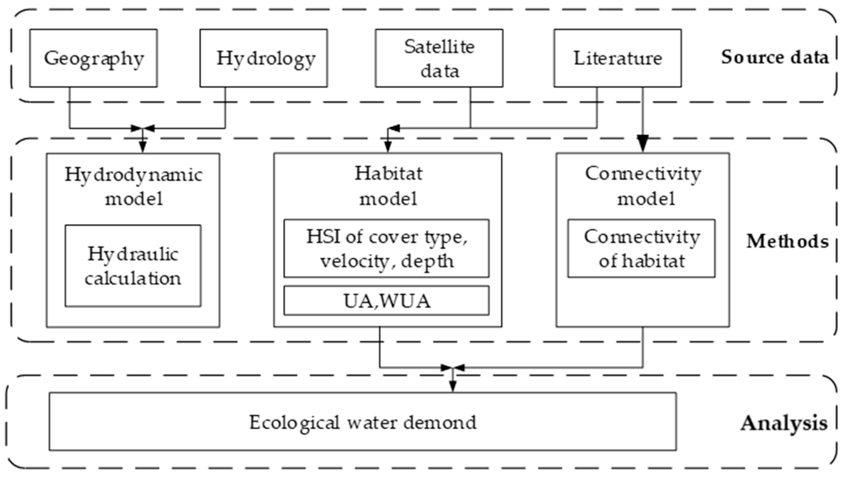
2. Materials and Methods
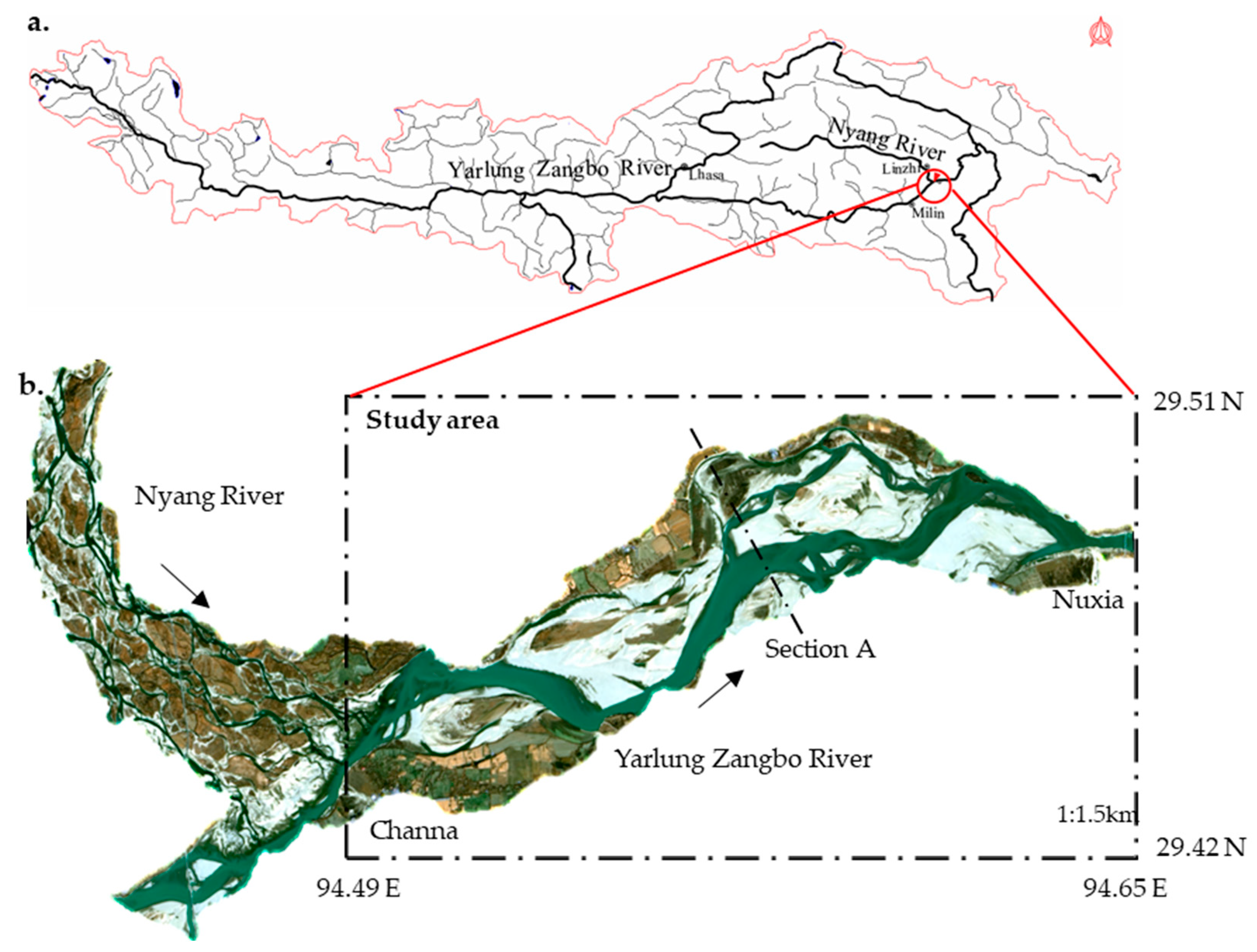
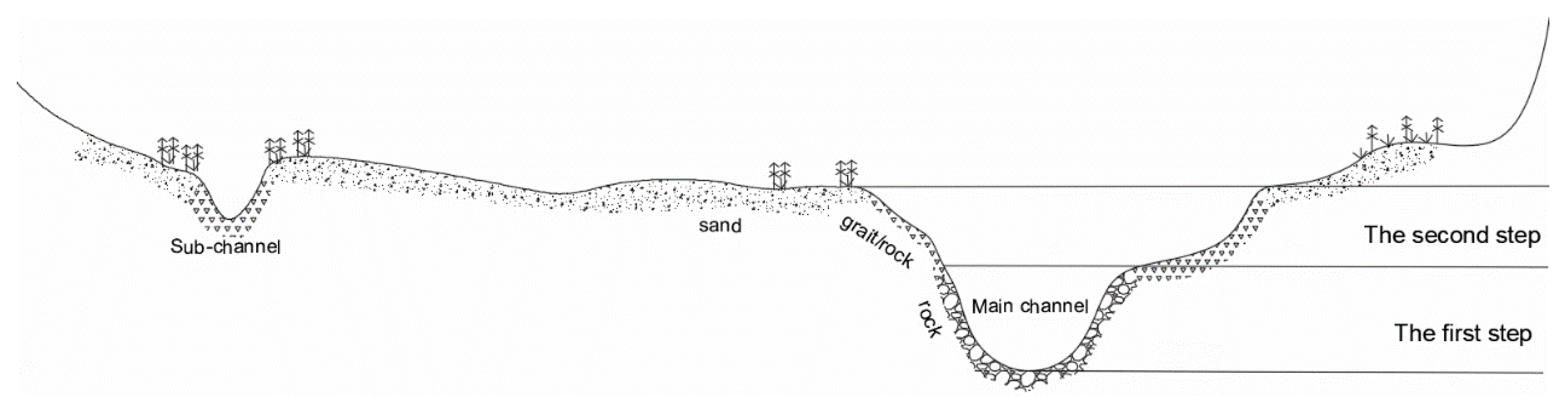
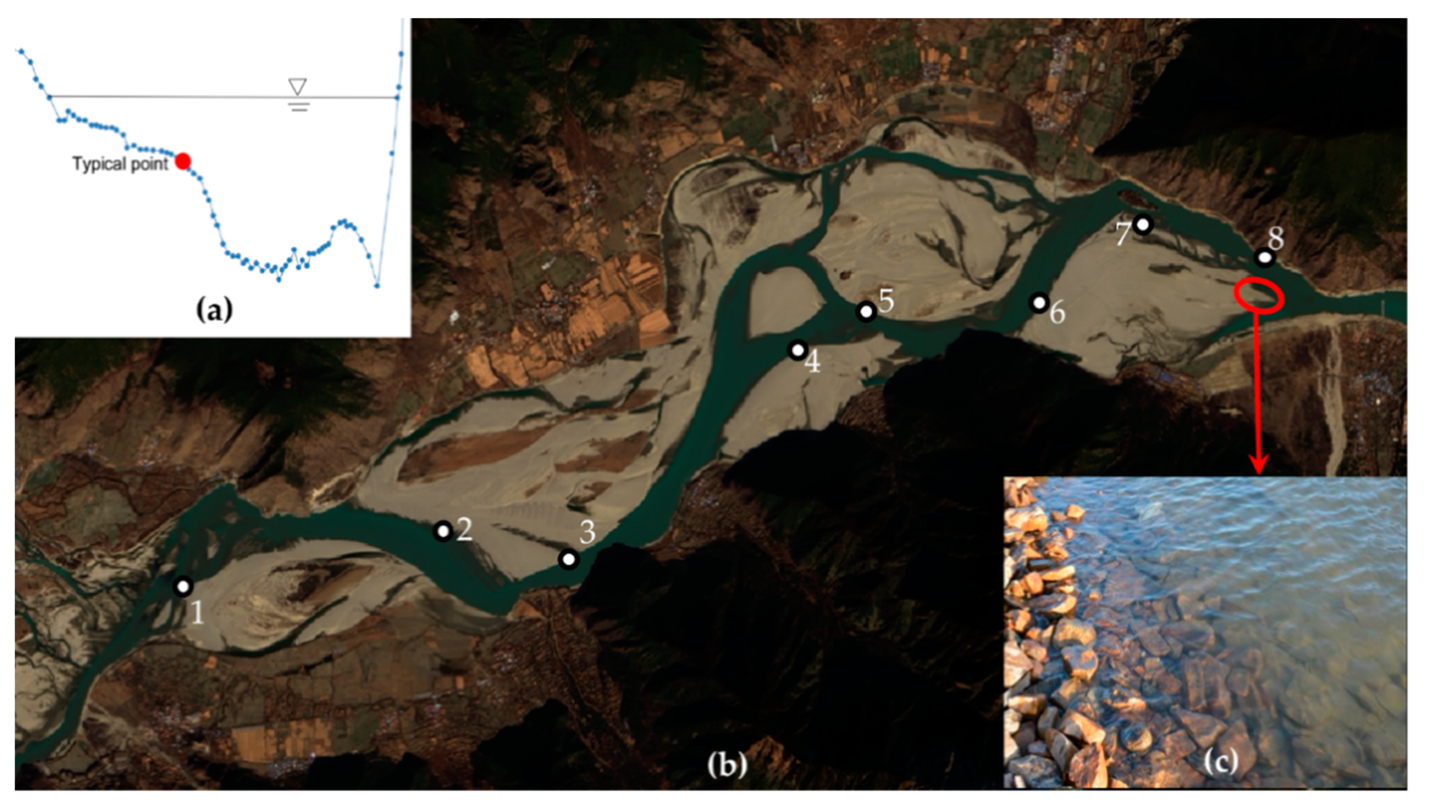
2.1. Study Area
2.2. Data
2.3. Methods
2.3.1. Hydrodynamic Model
- (a)
- Continuity equation:
- (b)
- Momentum equation:where η is the water level; d is the static water depth; h = η − d is the total water depth; u and v are the velocity components (m/s); is the Coriolis force, where ω is the rotational angular velocity of the earth and is the local latitude; g is the gravity (m2/s); ρ is the water density; Sxx, Sxy, and Syy are the respective radiation stress components; S is the source; us and vs are the velocity of the source, respectively; and Tij is the horizontal viscous stress term.
2.3.2. Habitat Model
2.3.3. Connectivity Model
3. Results
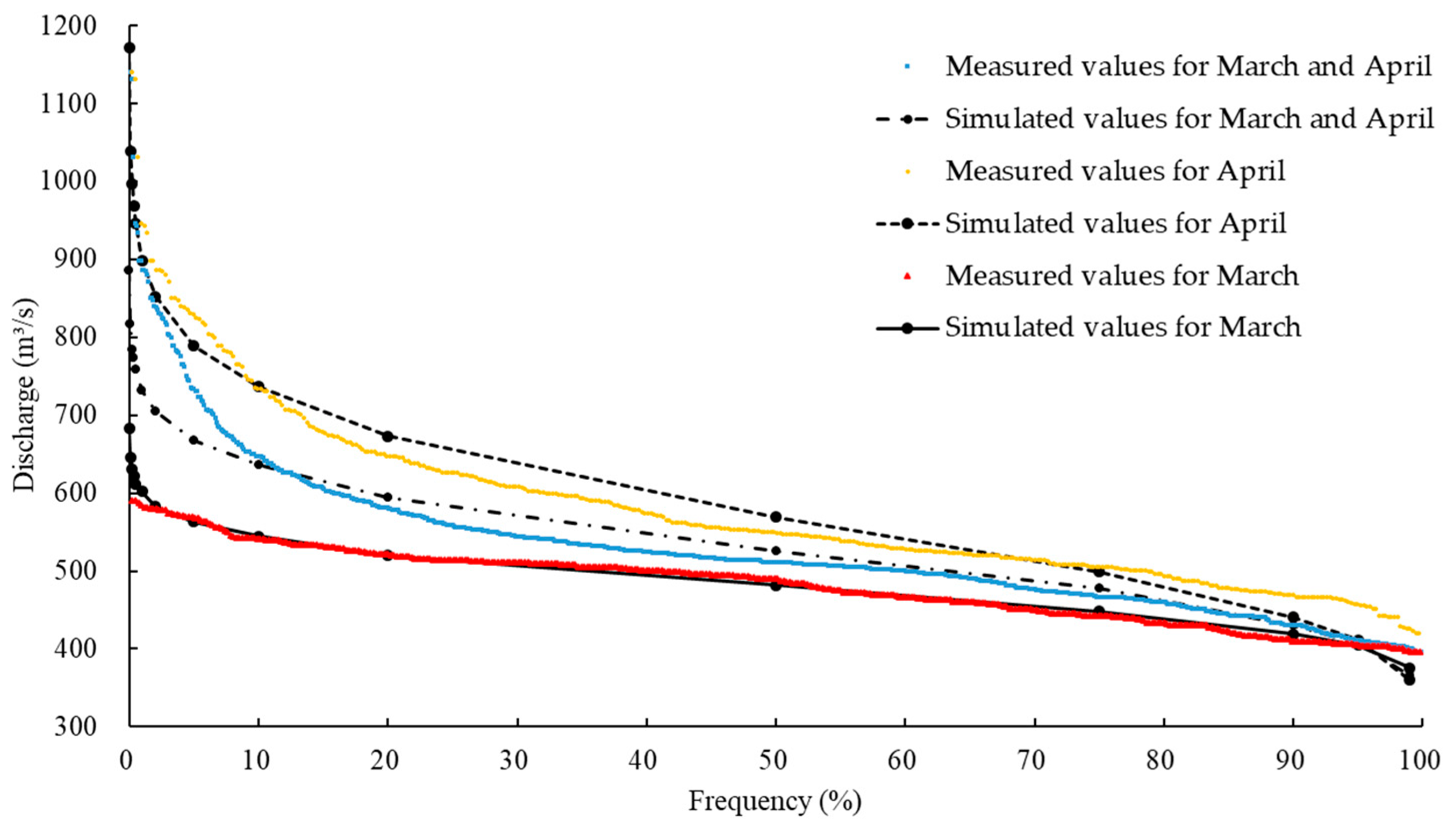
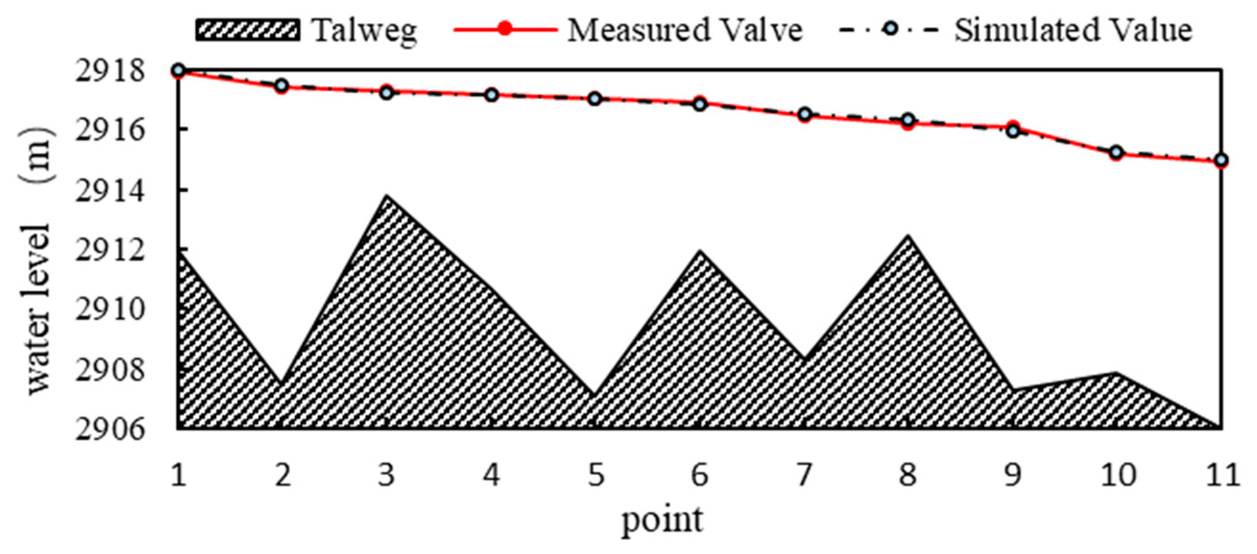
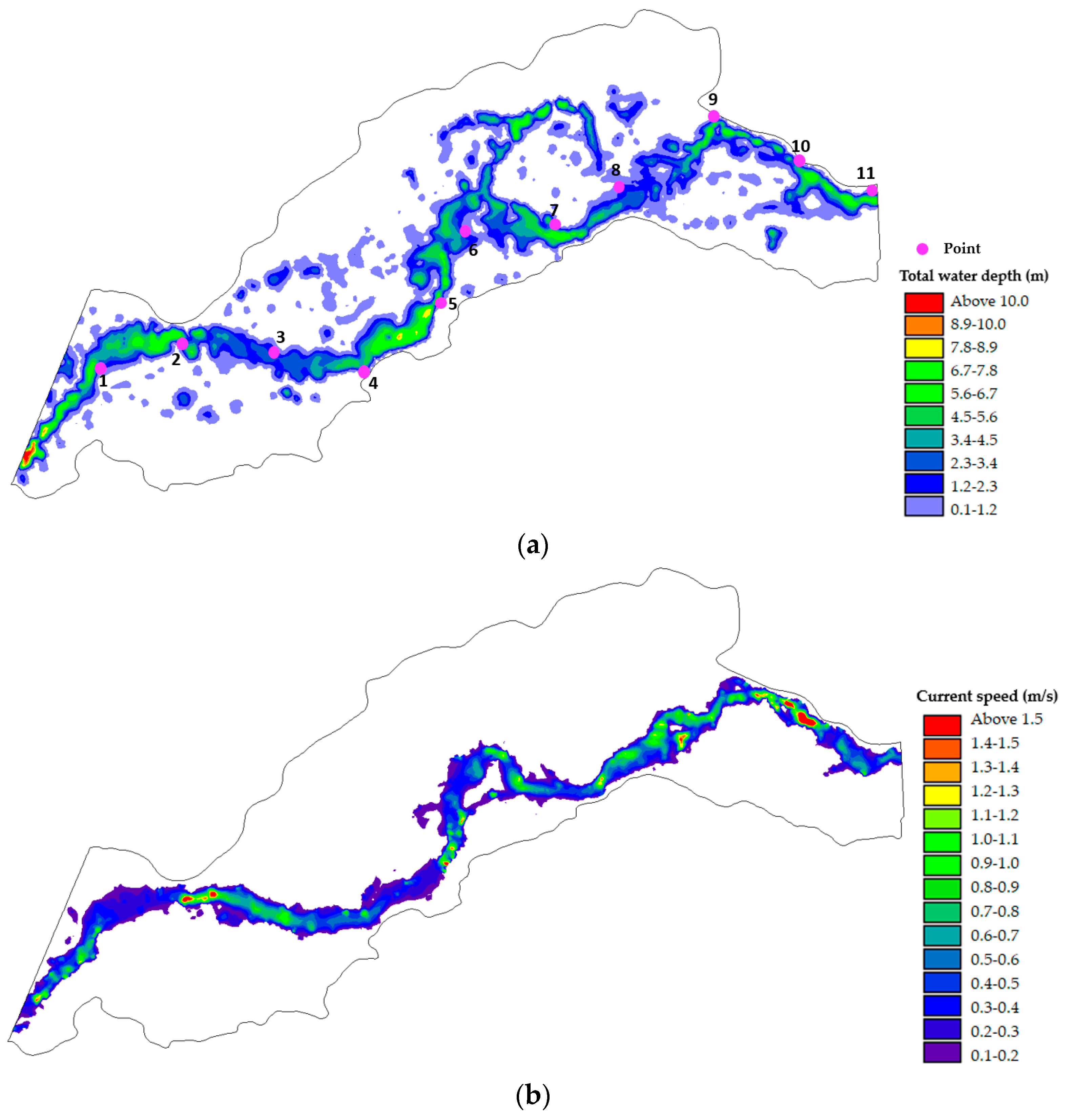
3.1. Hydrodynamic Model
3.2. Habitat Model
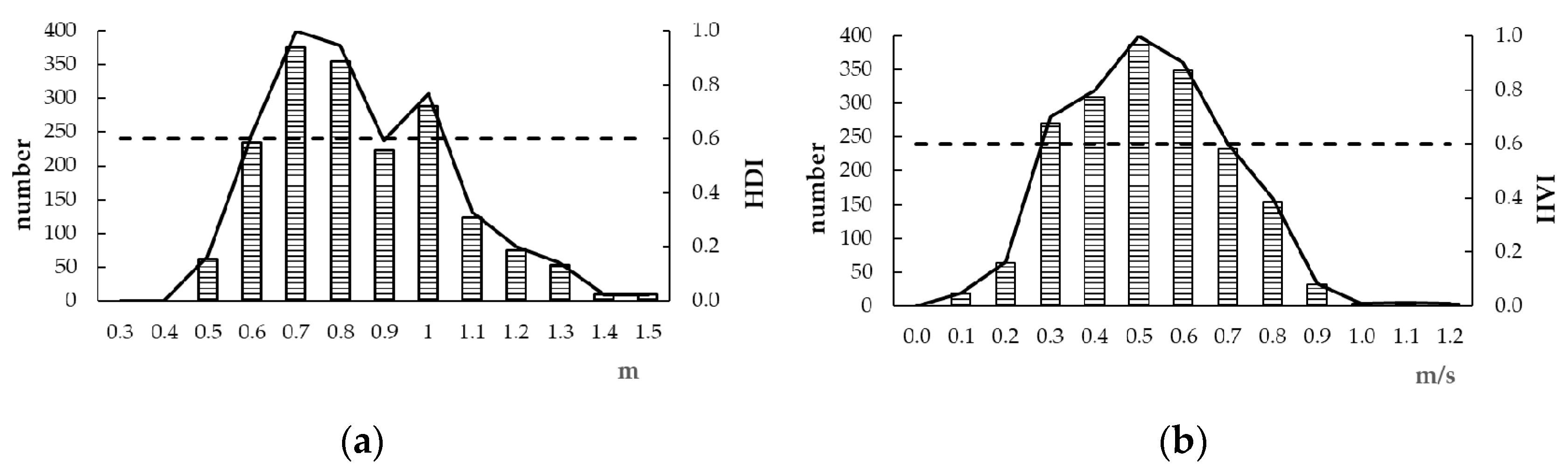
3.2.1. Habitat Suitability Index
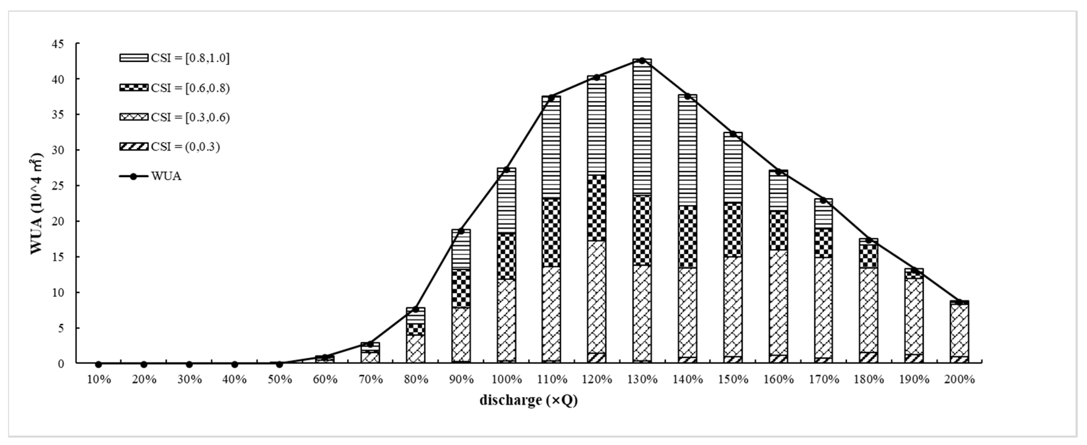
3.2.2. Suitable Area
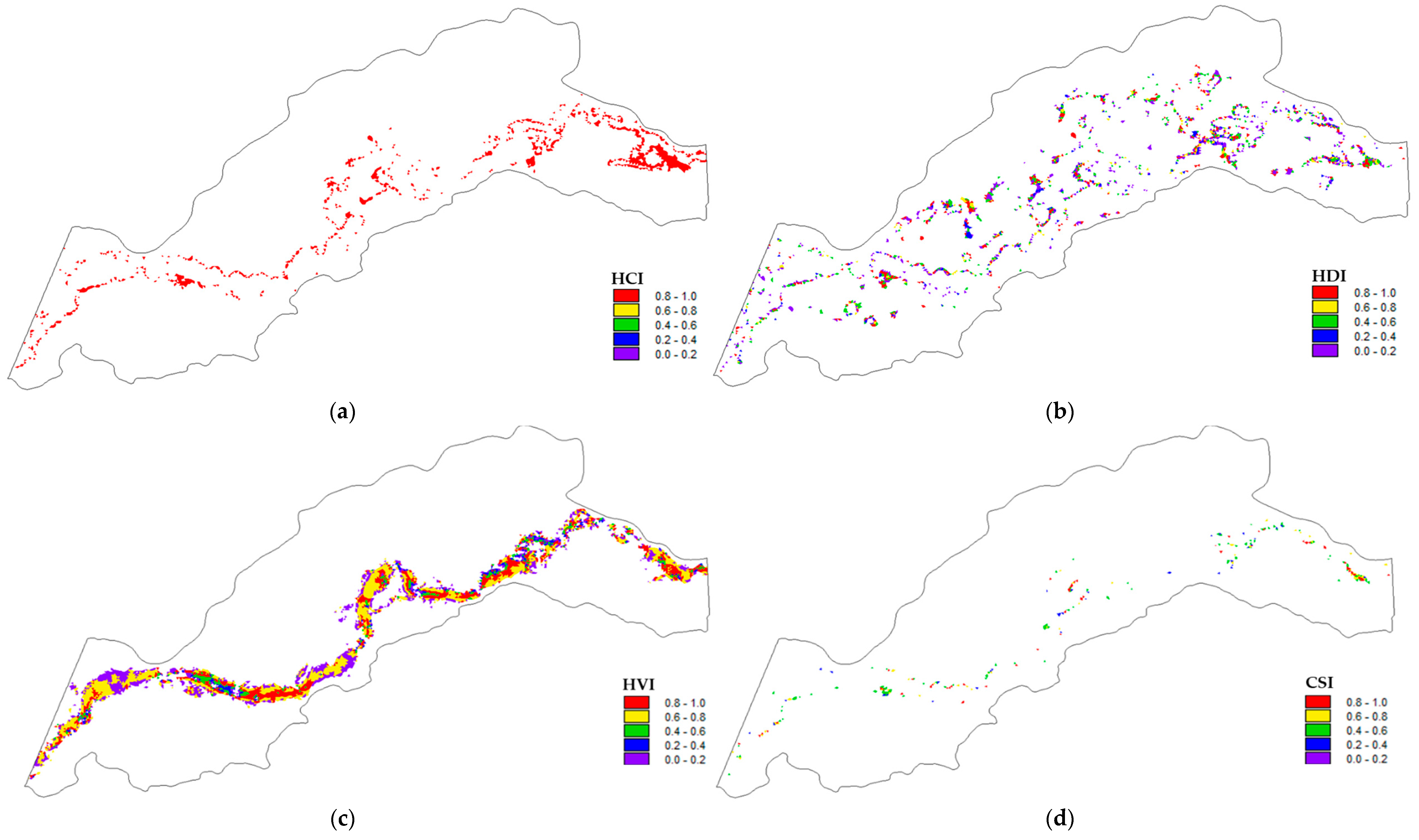
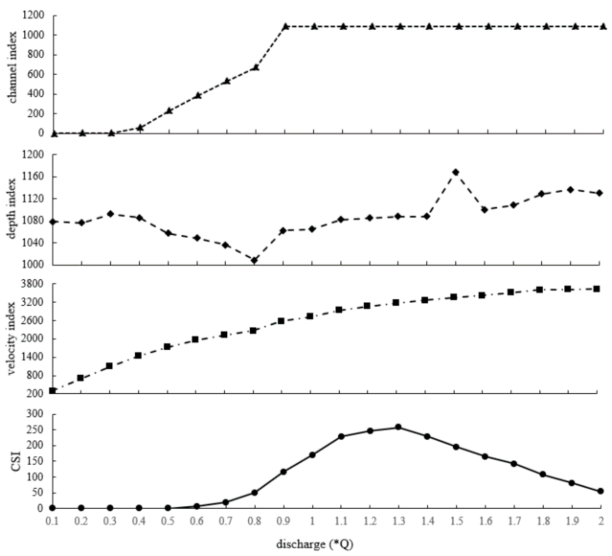
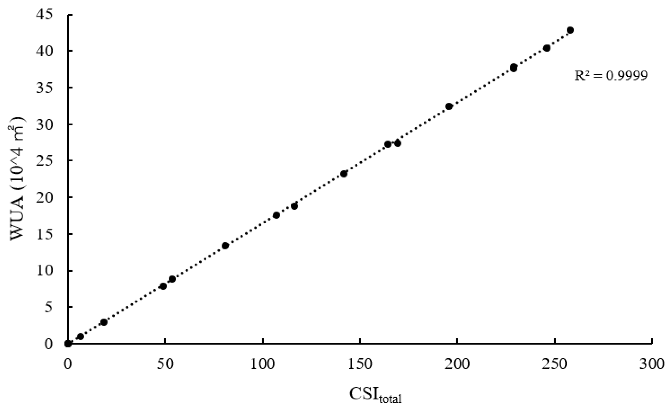
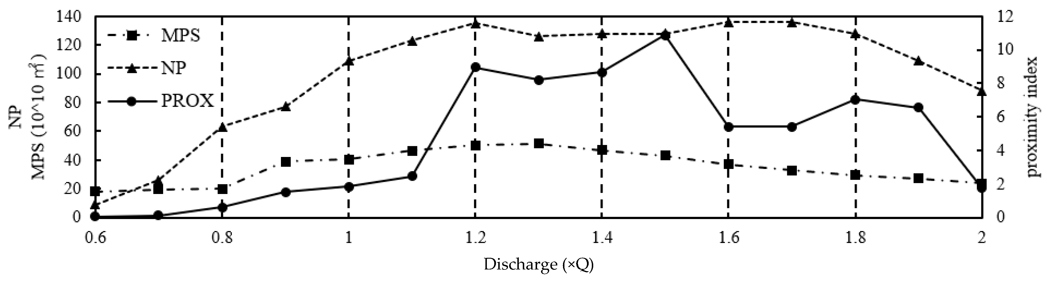
3.3. Connectivity Model
4. Discussion
5. Conclusions
- (1)
- The model results indicated that the suitable spawning habitat of Schizothorax is cobble with nearby sandy land. Additionally, the suitable water depth is 0.5–1.5 m, and the suitable velocity is 0.1–0.9 m/s. The results enrich the research on the HSI of Schizothorax in the Brahmaputra River.
- (2)
- When the runoff regulation flow was from 424–1060 m3/s, the WUA and connectivity satisfied the requirement for spawning under natural conditions with different habitat states.
- (3)
- When the runoff was from 424–530 m3/s or 848–1060 m3/s, the habitat quality generally satisfied the requirements for spawning. When the runoff was from 530–636 m3/s or 742–848 m3/s, the habitat was in a good state. When the runoff was from 636–742 m3/s, the habitat was in a best state.
Author Contributions
Funding
Acknowledgments
Conflicts of Interest
References
- Brown, C.M.; Lund, J.R.; Cai, X.; Reed, P.M. The future of water resources systems analysis: Toward a scientific framework for sustainable water management. Water Resour. Res. 2015, 51, 6110–6124. [Google Scholar] [CrossRef]
- Gerten, D.; Hoff, H.; Rockström, J.; Jägermeyr, J. Towards a revised planetary boundary for consumptive freshwater use: Role of environmental flow requirements. Curr. Opin. Environ. Sustain. 2013, 5, 551–558. [Google Scholar] [CrossRef]
- Wang, B.; Shao, D.G.; Mu, G.L.; Wang, Z.M. An eco-functional classification for environmental flow assessment in the Pearl River Basin in Guangdong, China. Sci. China Technol. Sci. 2016, 59, 265–275. [Google Scholar] [CrossRef]
- Abd-El, M.H.; Smith, S.E.; Darwish, K. Impacts of the Aswan High Dam After 50 Years. Water Resour. Manag. 2015, 29, 1873–1885. [Google Scholar] [CrossRef]
- Avery, L.A.; Korman, J.; Persons, W.R. Effects of Increased Discharge on Spawning and Age-0 Recruitment of Rainbow Trout in the Colorado River at Lees Ferry, Arizona. N. Am. J. Fish. Manag. 2015, 35, 671–680. [Google Scholar] [CrossRef]
- Liu, Z.; Yao, Z.; Huang, H.; Wu, S. Land use and climate changes and their impacts on runoff in the Yarlung Zangbo river basin, China. Land Degrad. Dev. 2014, 25, 203–215. [Google Scholar] [CrossRef]
- Mcowen, C.J.; Cheung, W.; Rykaczewski, R.R.; Watson, R. Is fisheries production within Large Marine Ecosystems determined by bottom-up or top-down forcing? Fish Fish. 2015, 16, 623–632. [Google Scholar] [CrossRef]
- Wang, B. The Research on the Method of Optimal Operation of Cascade Reservoirs Based on Suitable Habitats for River Fishes; Wuhan University: Wuhan, China, 2016. [Google Scholar]
- Wang, J.L.; Mou, Z.B.; Wang, Q.L. Research Progress on Schizothoracinae Fishes in Tibet. Anhui Agric. Sci. 2018, 46, 16–19. [Google Scholar]
- Zhou, X.J. Study on the Biology and Population Dynamics of Schizothorax waltoni; Huazhong Agricultural University: Wuhan, China, 2014. [Google Scholar]
- Ye, F.L.; Zhang, J.D. Fish Ecology; Guangdong Higher Education Press: Guangzhou, China, 2002. [Google Scholar]
- Ma, B.S. Study on the Biology and Population Dynamics of Schizothorax o’connori; Huazhong Agricultural University: Wuhan, China, 2011. [Google Scholar]
- Tharme, R.E. A global perspective on environmental flow assessment: Emerging trends in the development and application of environmental flow methodologies for rivers. River Res. Appl. 2003, 19, 397–441. [Google Scholar]
- Reiser, D.W.; Wesche, T.A.; Estes, C. Status of Instream Flow Legislation and Practices in North America. Fisheries 1989, 14, 22–29. [Google Scholar] [CrossRef]
- Zabet, S. A Comparison of 7Q10 Low Flow between Rural and Urban Watersheds in Eastern United States. Master’s Thesis, University of Tennessee, Knoxville, TN, USA, 2012. [Google Scholar]
- Jha, R.; Sharma, K.D.; Singh, V.P. Critical appraisal of methods for the assessment of environmental flows and their application in two river systems of India. Ksce J. Civ. Eng. 2008, 12, 213–219. [Google Scholar] [CrossRef]
- Liu, C.; Zhao, C.; Xia, J.; Sun, C.; Wang, R.; Liu, T. An instream ecological flow method for data-scarce regulated rivers. J. Hydrol. (Amst.) 2011, 398, 17–25. [Google Scholar] [CrossRef]
- Barrett, M.P.J. An Evaluation of the Instream Flow Incremental Methodology (IFIM). J. Ariz.-Nev. Acad. Sci. 1992, 24–25, 75–77. [Google Scholar]
- Leclerc, M.; Boudreault, A.; Bechara, T.A.; Corfa, G. Two-Dimensional Hydrodynamic Modeling: A Neglected Tool in the Instream Flow Incremental Methodology. Trans. Am. Fish. Soc. 1995, 124, 645–662. [Google Scholar] [CrossRef]
- Petts, G.E. Water allocation to protect river ecosystems. Regul. Rivers Res. Manag. 1996, 12, 353–365. [Google Scholar] [CrossRef]
- Gore, J.A.; Crawford, D.J.; Addison, D.S. An analysis of artificial riffles and enhancement of benthic community diversity by physical habitat simulation (PHABSIM) and direct observation. River Res. Appl. 2015, 14, 69–77. [Google Scholar] [CrossRef]
- Nicolas, L.; Jowett, I.G. Generalized instream habitat models. Can. J. Fish. Aquat. Sci. 2005, 62, 7–14. [Google Scholar]
- Gallagher, S.P. Use of Two Dimensional Hydrodynamic Modelling to Evaluate Channel Rehabilitation in the Trinity River, California; USAUS Fish and Wildlife Service, Arcata Fish and Wildlife Office: Arcata, CA, USA, 1999. [Google Scholar]
- Lamouroux, N.; Oliver, J.M.; Persat, H.; Pouilly, M. Predicting Community Characteristics from Habitat Conditions: Fluvial Fish and Hydraulics. Freshw. Biol. 1999, 42, 275–299. [Google Scholar] [CrossRef]
- Moir, H.J.; Soulsby, C.; Youngson, A. Hydraulic and sedimentary characteristics of habitat utilized by Atlantic salmon for spawning in the Girnock Burn, Scotland. Fish. Manag. Ecol. 2010, 5, 241–254. [Google Scholar] [CrossRef]
- Wang, Y.K.; Xia, Z.Q. Three-dimensional Hydraulics Characteristics of Chinese Sturgeon Spawning Site in the Yangtze River. J. Sichuan Univ. (Eng. Sci. Ed.) 2010, 42, 14–19. [Google Scholar]
- Li, J.; Xia, Z.Q.; Wang, Y.K.; Zheng, Q. Study on River Morphology and Flow Characteristics of Four Major ChineseCarps Spawning Grounds in the Middle Reach of the Yangtze River. J. Sichuan Univ. (Eng. Sci. Ed.) 2010, 42, 63–70. [Google Scholar]
- Crowder, D.W.; Diplas, P. Evaluating spatially explicit metrics of stream energy gradients using hydrodynamic model simulations. Can. J. Fish. Aquat. Sci. 2000, 57, 1497–1507. [Google Scholar] [CrossRef]
- Crowder, D.W.; Diplas, P. Vorticity and circulation: Spatial metrics for evaluating flow complexity in stream habitats. Can. J. Fish. Aquat. Sci. 2002, 59, 633–645. [Google Scholar] [CrossRef]
- Sang, L.H.; Chen, X.Q.; Huang, W. Evolution of environmental flow methodologies for rivers. Adv. Water Sci. 2006, 17, 754–760. [Google Scholar]
- Wiens, J.A. Riverine landscapes: Taking landscape ecology into the water. Freshw. Biol. 2010, 47, 501–515. [Google Scholar] [CrossRef]
- Carnie, R.; Tonina, D.; Mckean, J.A.; Isaak, D.J. Habitat connectivity as a metric for aquatic microhabitat quality: Application to Chinook salmon spawning habitat. Ecohydrology 2015, 9, 982–994. [Google Scholar] [CrossRef]
- Le Pichon, C.; Gorges, G.; Baudry, J.; Goreaud, F.; Boët, P. Spatial metrics and methods for riverscapes: Quantifying variability in riverine fish habitat patterns. Environmetrics 2009, 20, 512–526. [Google Scholar] [CrossRef]
- Zhu, T.B.; Chen, L.; Yang, D.G.; Ma, B.; Li, L. Distribution and habitat character of Schizothoracine fishes in the middle Yarlung Zangbo river. Chin. J. Ecol. 2017, 36, 2817–2823. [Google Scholar]
- Wang, S.; Jie, Y. China Species Red List; Higher Education Press: Beijing, China, 2004. [Google Scholar]
- Zhu, C.J.; Liang, Q.; Yan, F.; Hao, W.L. Reduction of Waste Water in Erhai Lake Based on MIKE21 Hydrodynamic and Water Quality Model. Sci. World J. 2013, 2013. [Google Scholar] [CrossRef]
- Chubarenko, I.; Tchepikova, I. Modelling of man-made contribution to salinity increase into the Vistula Lagoon (Baltic Sea). Ecol. Model. 2001, 138, 87–100. [Google Scholar] [CrossRef]
- Xu, M.J.; Yu, L.; Zhao, Y.W.; Li, M. The Simulation of Shallow Reservoir Eutrophication Based on MIKE21: A Case Study of Douhe Reservoir in North China. Procedia Environ. Sci. 2012, 13, 1975–1988. [Google Scholar] [CrossRef] [Green Version]
- Duong, T.A.; Long, P.H.; Minh, D.B.; Peter, R. Simulating Future Flows and Salinity Intrusion Using Combined One- and Two-Dimensional Hydrodynamic Modelling—The Case of Hau River, Vietnamese Mekong Delta. Water 2018, 10, 897. [Google Scholar]
- Lin, J.Q.; Peng, Q.D.; Huang, Z.L. Review on hydraulics research of fish eggs’ movement in rivers. J. Hydraul. Eng. 2015, 46, 869–876. [Google Scholar]
- Hampton, H. Development of Habitat Preference Criteria for Anadromous Salmonids of the Trinity River; US Fish & Wildlife Service, Division of Ecological Services: Sacramento, CA, USA, 1988; 93p.
- Ding, R.H. The Fishes of Sichuan, China; Sichuan Publishing House of Science and Technology: Chengdu, China, 1994. [Google Scholar]
- Cao, W.X.; Chang, J.B.; Qian, Y.; Duan, Z.H. Fish Resource of Early Life History Stages in Yangtze River; China Waterpower Press: Beijing, China, 2007. [Google Scholar]
- Gustafson, E.J.; Parker, G.R. Using an index of habitat patch proximity for landscape design. Landsc. Urban Plan. 1994, 29, 117–130. [Google Scholar] [CrossRef]
- Zhang, Z.G.; Tan, Q.L.; Zhong, Z.G.; Jin, Y.; Du, J. study on ecological flow regime based on habitat requirement of fish. Water Power 2016, 42, 13–17. [Google Scholar]
- Gard, M. Comparison of spawning habitat predictions of PHABSIM and River2D models. Int. J. River Basin Manag. 2009, 7, 55–71. [Google Scholar] [CrossRef]
- Fu, J.J.; Huang, B.; Rui, J.L.; Tan, S.K.; Zhao, S. Application of Habitat Simulation to Fishery Habitat Protection in Heishui River. J. Hydroecol. 2016, 37, 70–75. [Google Scholar]
- Yang, Z.F.; Yu, S.W.; Chen, H.; She, D.X. Model for defining environmental flow thresholds of spring flood period using abrupt habitat change analysis. Adv. Water Sci. 2010, 21, 567–574. [Google Scholar]


| Class | CSI 1 Range | Suitability Level |
|---|---|---|
| a | 1.0 > CSI > 0 | Total habitat, including all suitable areas |
| b1 | 0.3 > CSI > 0 | Poor habitat |
| b2 | 0.6 > CSI > 0.3 | Intermediate habitat |
| b3 | 0.8 > CSI > 0.6 | Good habitat |
| b4 | 1.0 > CSI > 0.8 | Best habitat |
| ×Q 1 | Habitat State | Corresponding Flow (m3/s) | |
|---|---|---|---|
| WUA 2 | 0.8–1 | Generally satisfactory | 530≥; ≥424 |
| 1–1.1 | Good state | 583>; ≥530 | |
| 1.1–1.4 | Best state | 742>; ≥583 | |
| 1.4–1.6 | Good state | 848>; ≥742 | |
| 1.6–2.0 | Generally satisfactory | 1060>; ≥848 | |
| Connectivity | 0.8–1.1 | Generally satisfactory | 583≥; ≥424 |
| 1.1–1.2 | Good state | 636>; ≥583 | |
| 1.2–1.5 | Best state | 795≥; ≥636 | |
| 1.5–1.9 | Good state | 1007≥; >795 | |
| 1.9–2.0 | Generally satisfactory | 1060≥; >1007 | |
| Overall consideration | 0.8–1.0 | Generally satisfactory | 530≥; ≥424 |
| 1.0–1.2 | Good state | 636>; ≥530 | |
| 1.2–1.4 | Best state | 742>; ≥636 | |
| 1.4–1.6 | Good state | 848>; ≥742 | |
| 1.6–2.0 | Generally satisfactory | 1060≥; ≥848 |
© 2019 by the authors. Licensee MDPI, Basel, Switzerland. This article is an open access article distributed under the terms and conditions of the Creative Commons Attribution (CC BY) license (http://creativecommons.org/licenses/by/4.0/).
Share and Cite
Zhou, Z.; Deng, Y.; Li, Y.; An, R. The Ecological Water Demand of Schizothorax in Tibet Based on Habitat Area and Connectivity. Int. J. Environ. Res. Public Health 2019, 16, 3045. https://0-doi-org.brum.beds.ac.uk/10.3390/ijerph16173045
Zhou Z, Deng Y, Li Y, An R. The Ecological Water Demand of Schizothorax in Tibet Based on Habitat Area and Connectivity. International Journal of Environmental Research and Public Health. 2019; 16(17):3045. https://0-doi-org.brum.beds.ac.uk/10.3390/ijerph16173045
Chicago/Turabian StyleZhou, Zili, Yun Deng, Yong Li, and Ruidong An. 2019. "The Ecological Water Demand of Schizothorax in Tibet Based on Habitat Area and Connectivity" International Journal of Environmental Research and Public Health 16, no. 17: 3045. https://0-doi-org.brum.beds.ac.uk/10.3390/ijerph16173045