Effect of Topographic Data Accuracy on Watershed Management


Abstract
:1. Introduction
2. Materials and Methods
2.1. Watershed Management Models
2.1.1. Watershed Modeling System (WMS)
2.1.2. Global Mapper
2.1.3. Google Earth Program
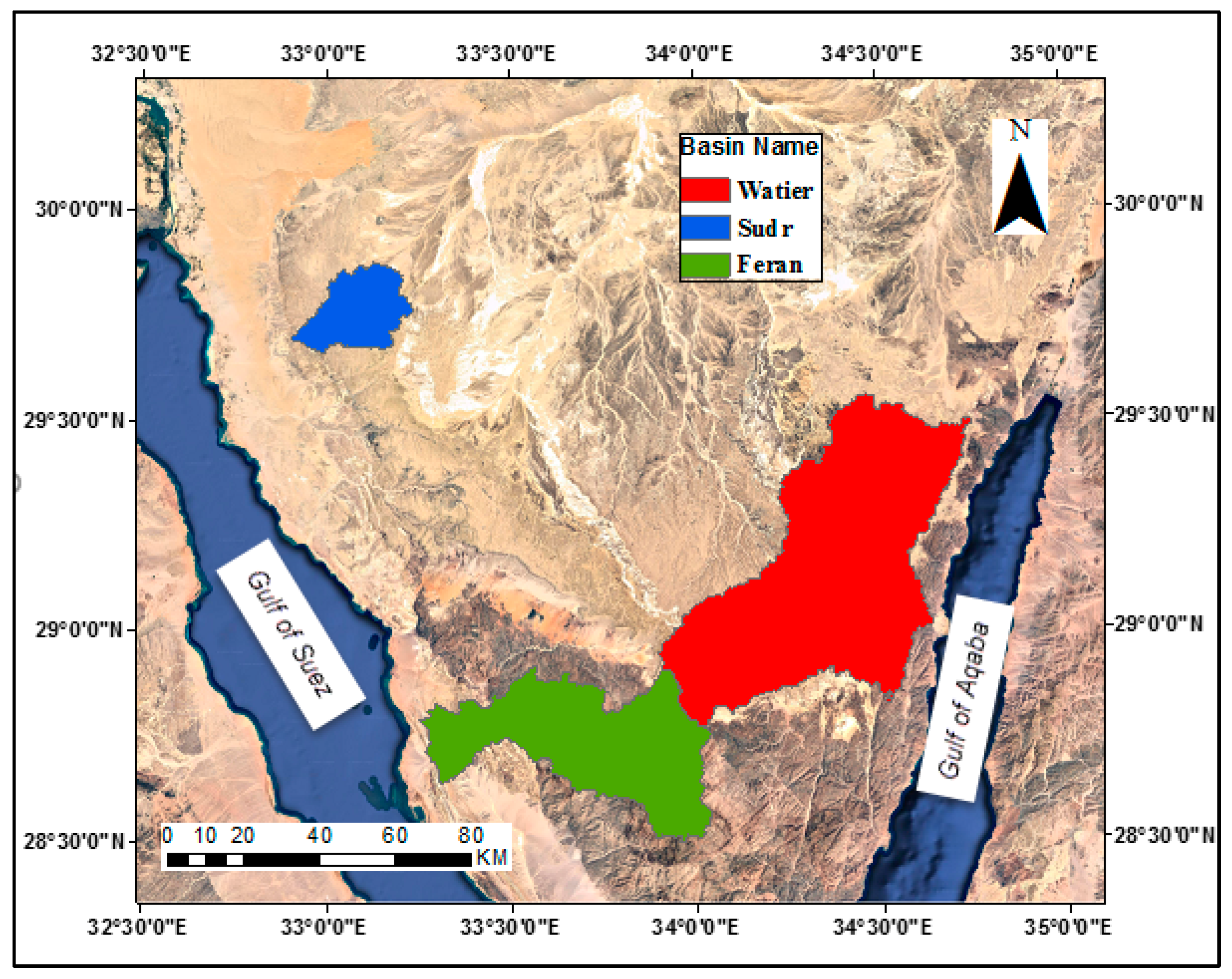
2.2. Case Studies
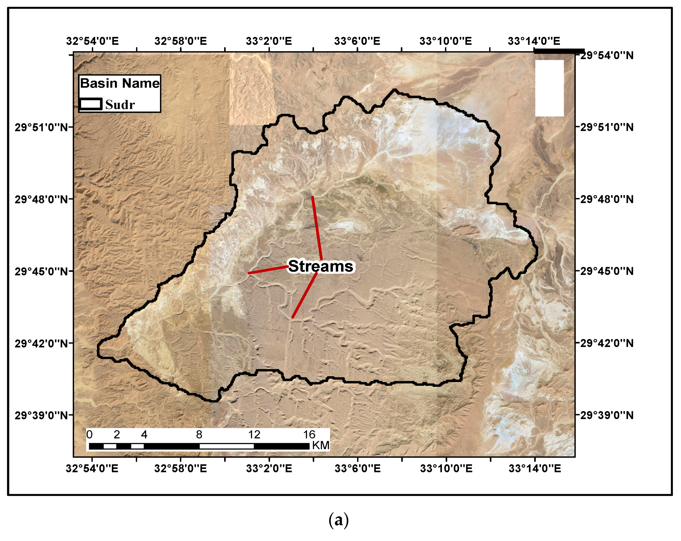
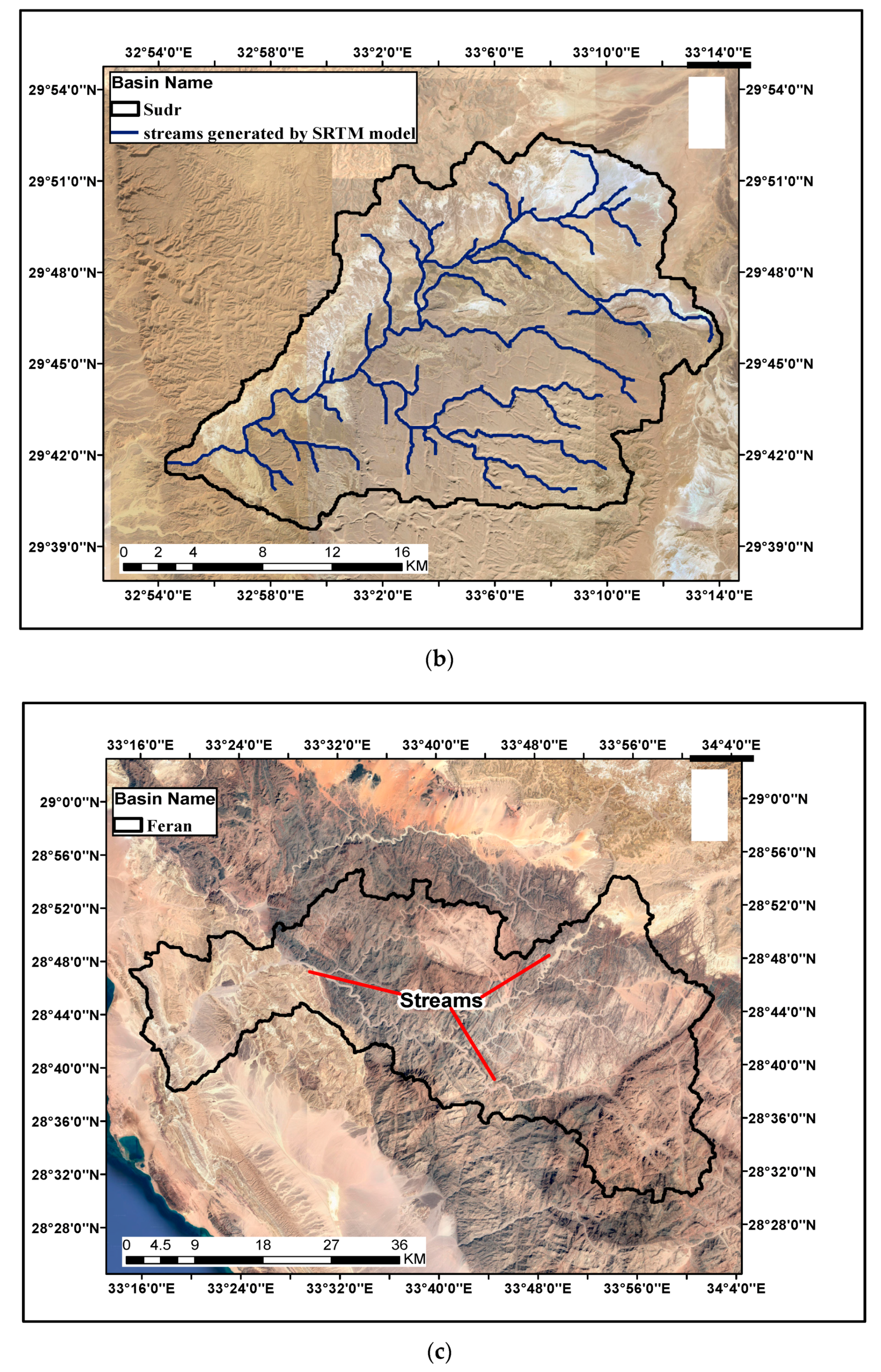
2.2.1. Wadi Sudr
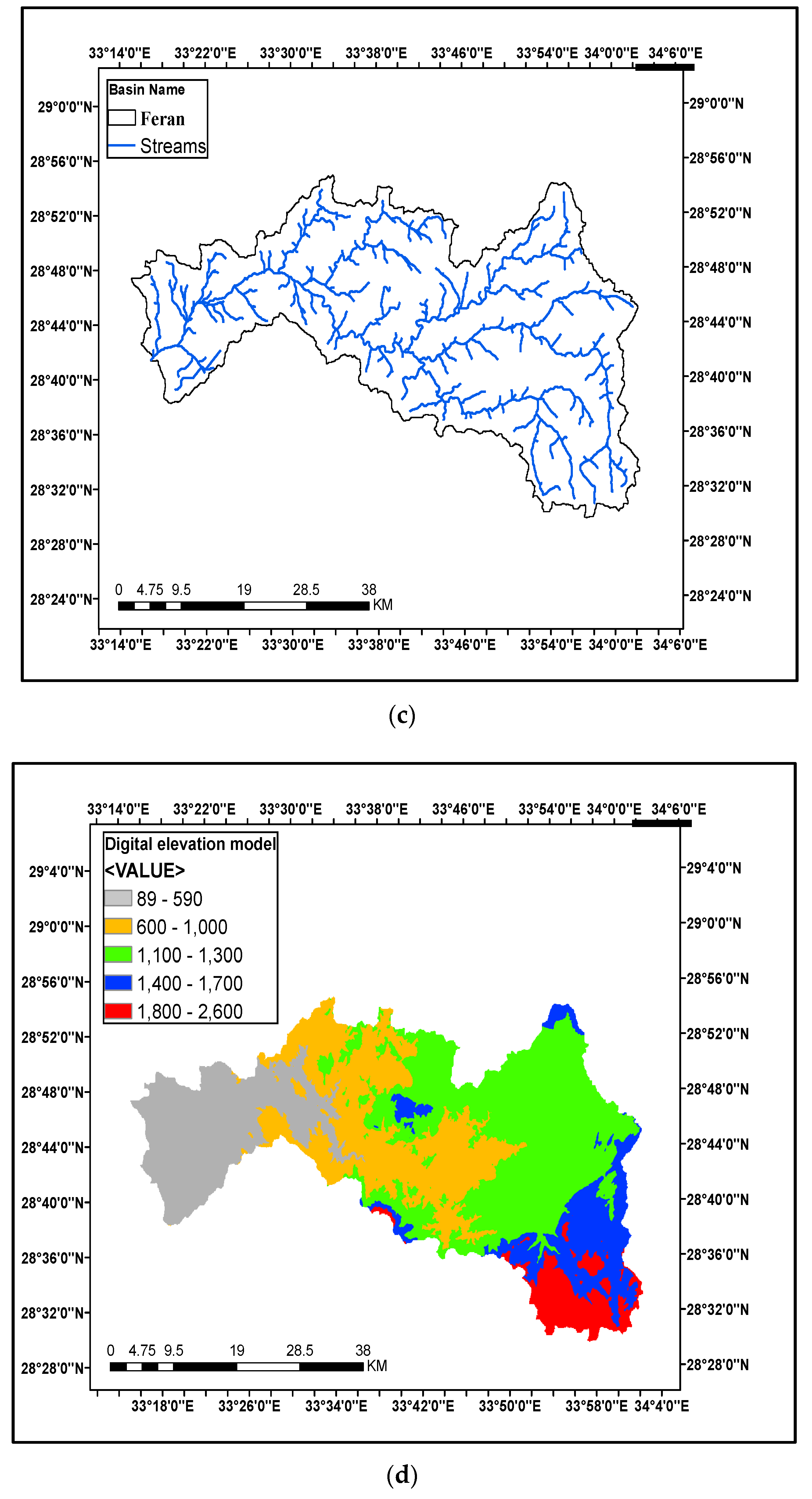
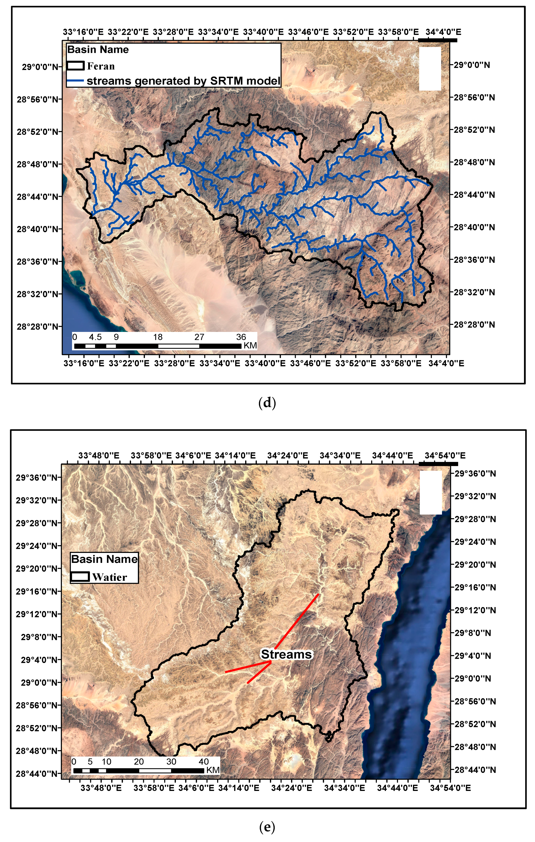
2.2.2. Wadi Feran
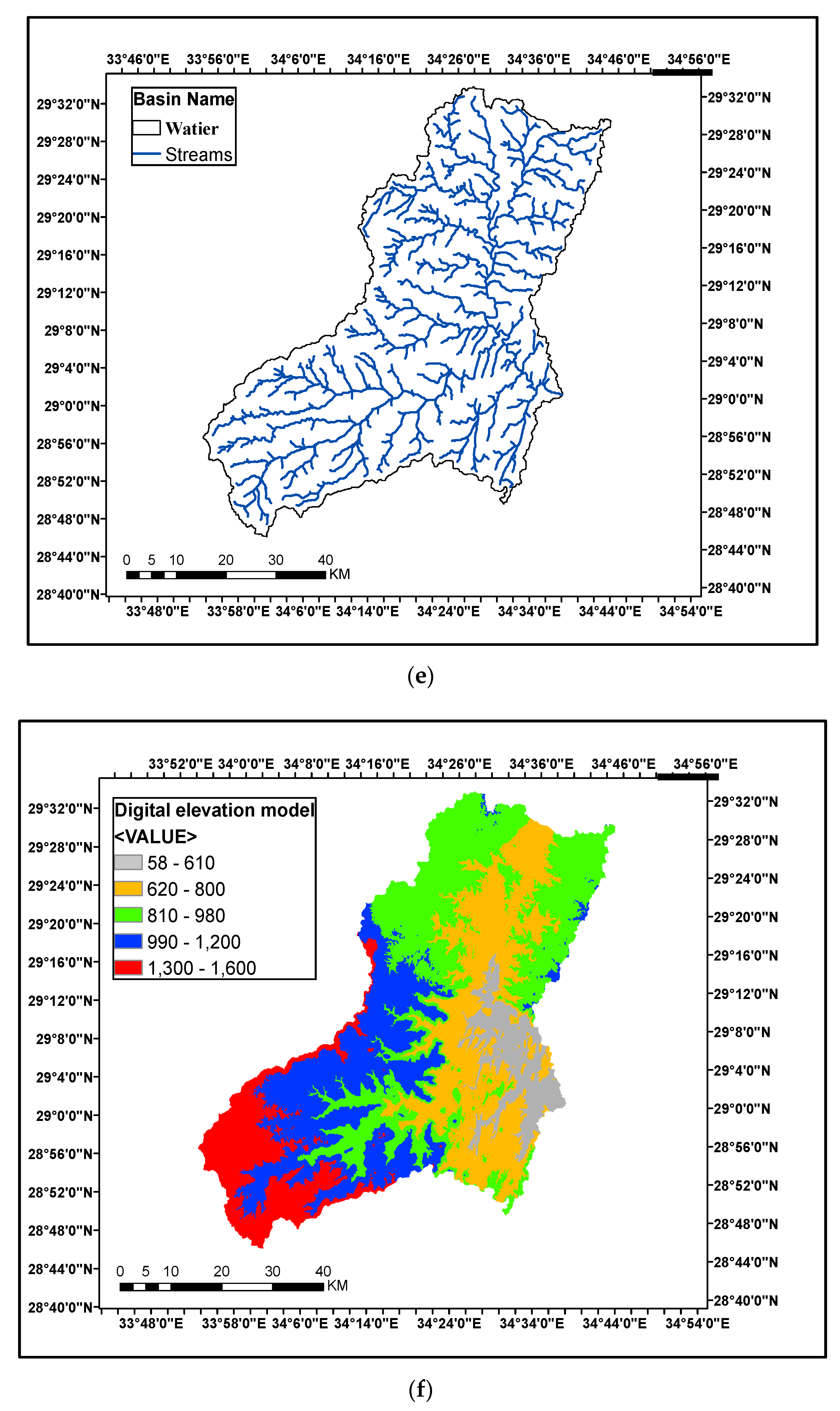
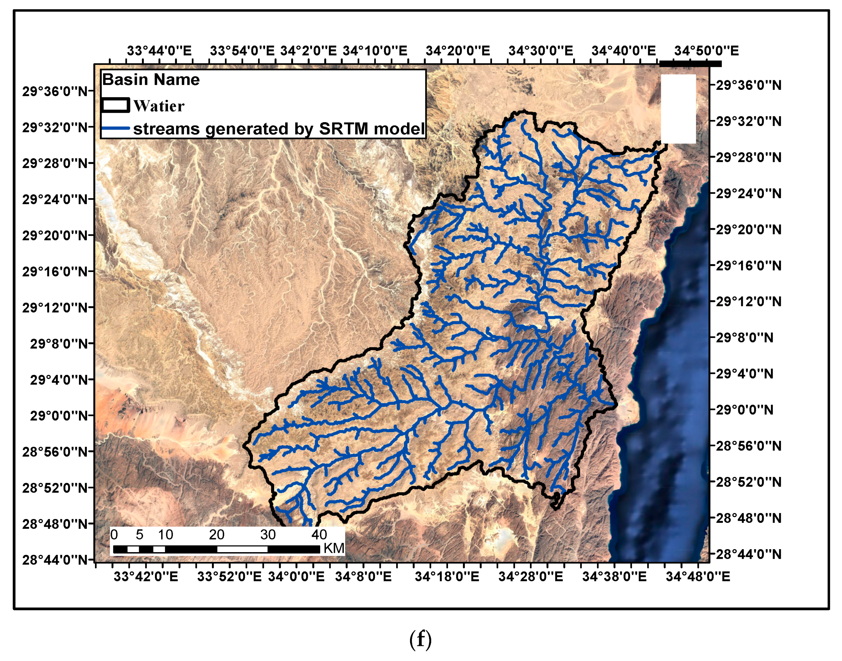
2.2.3. Wadi Watier
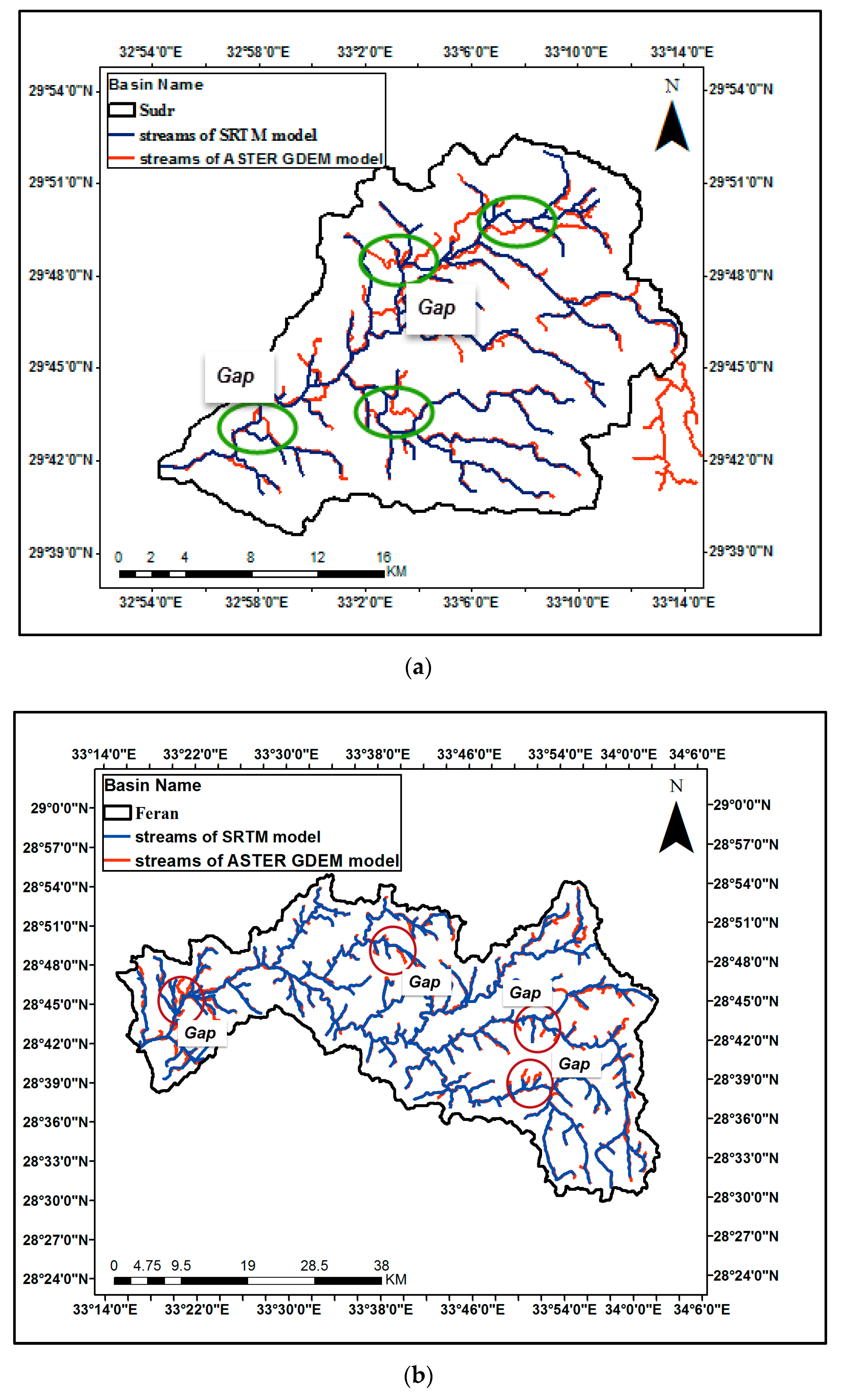
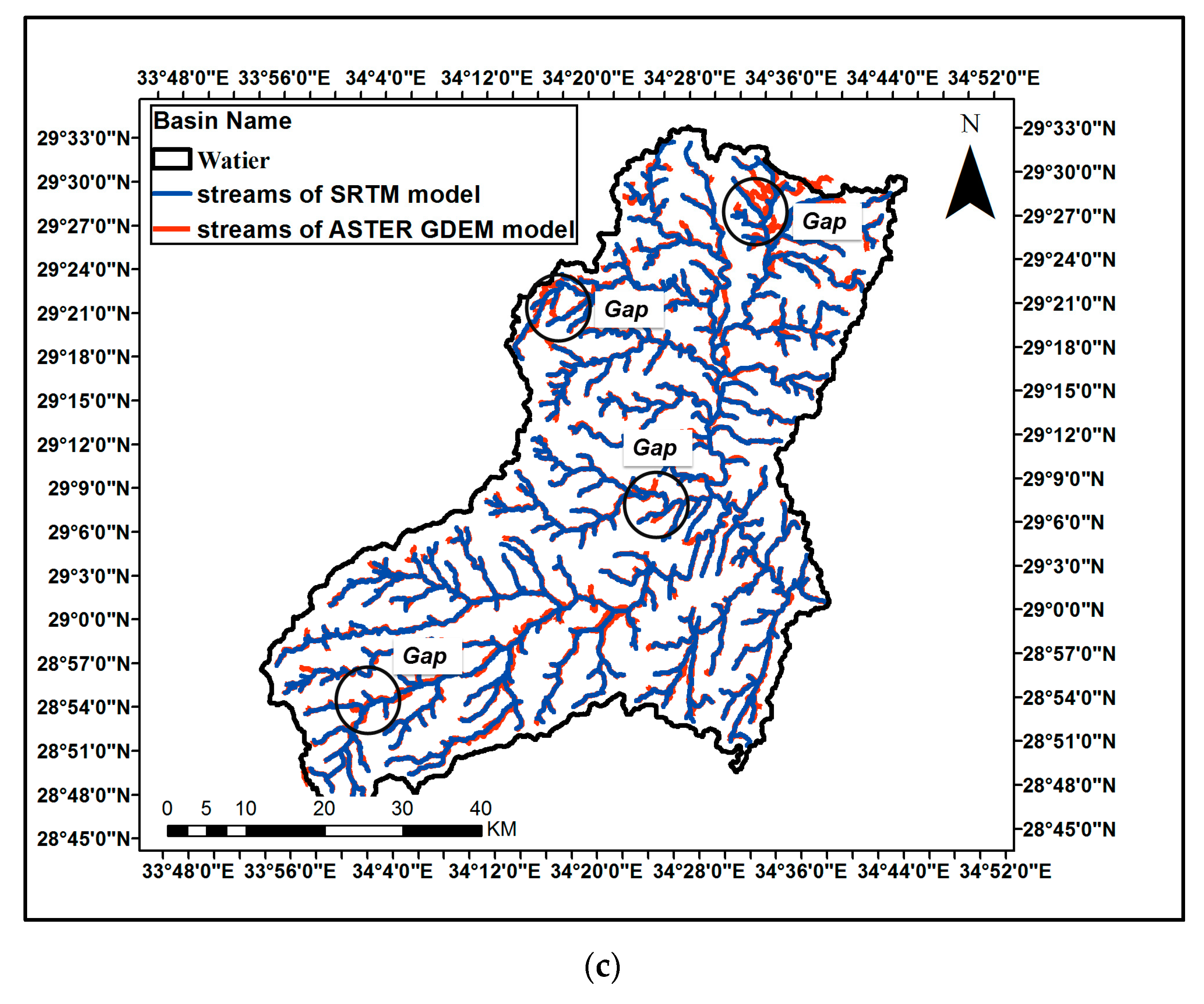
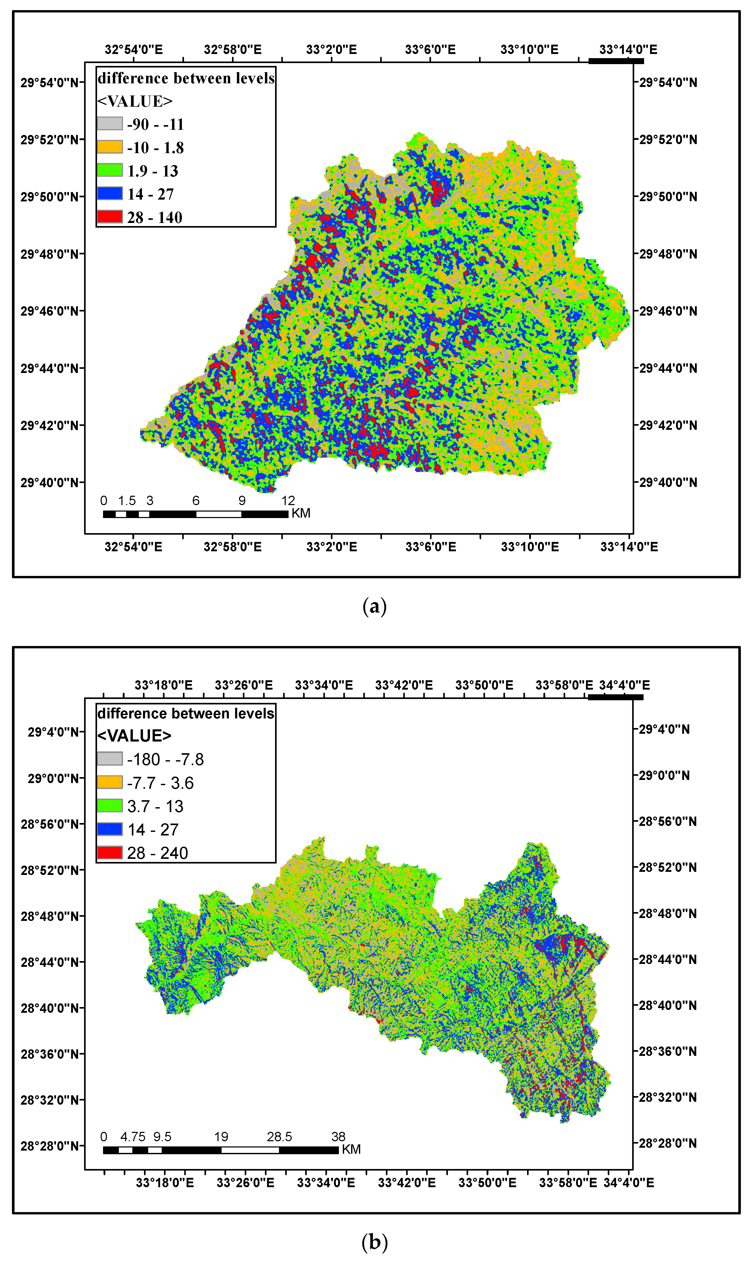
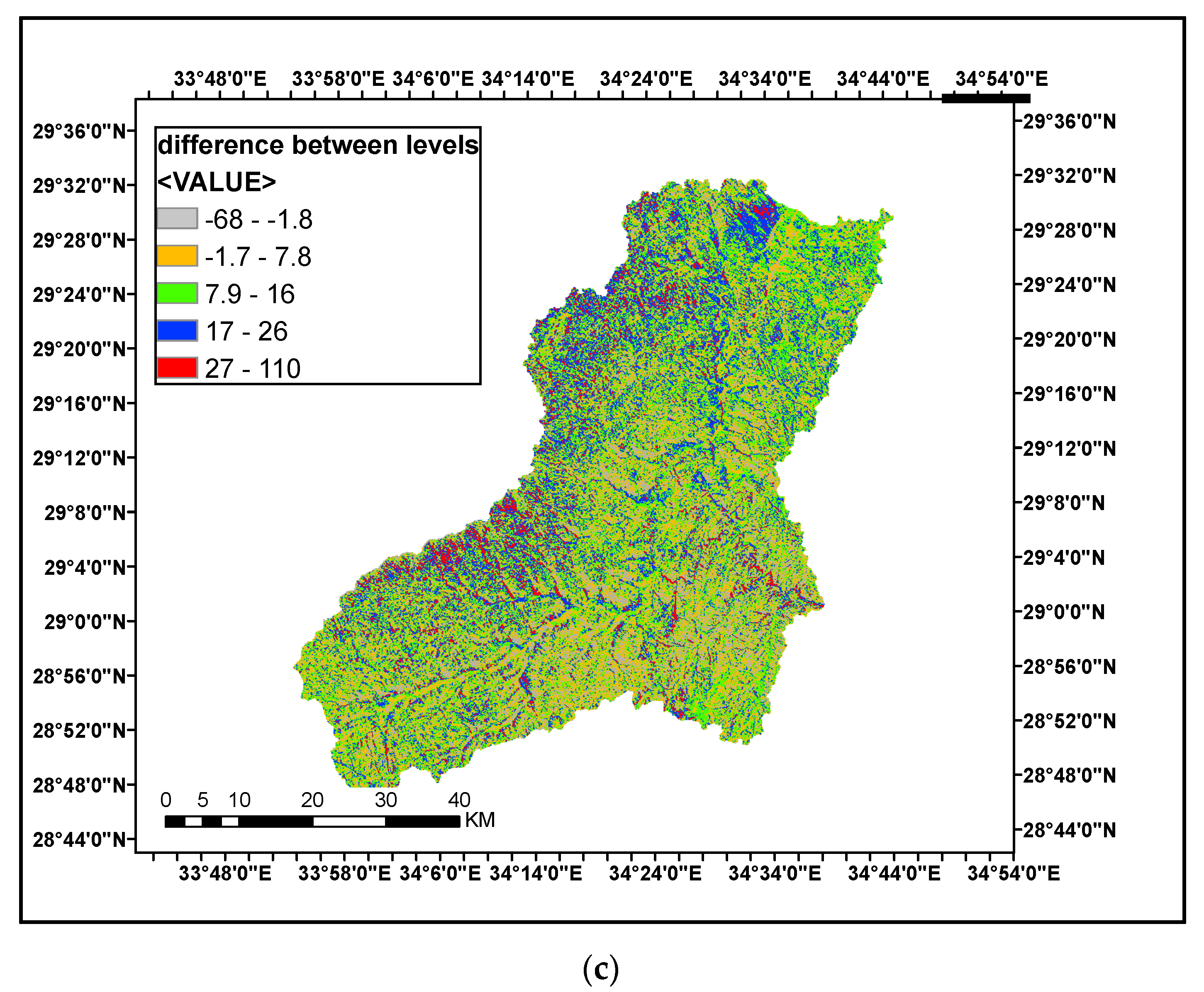
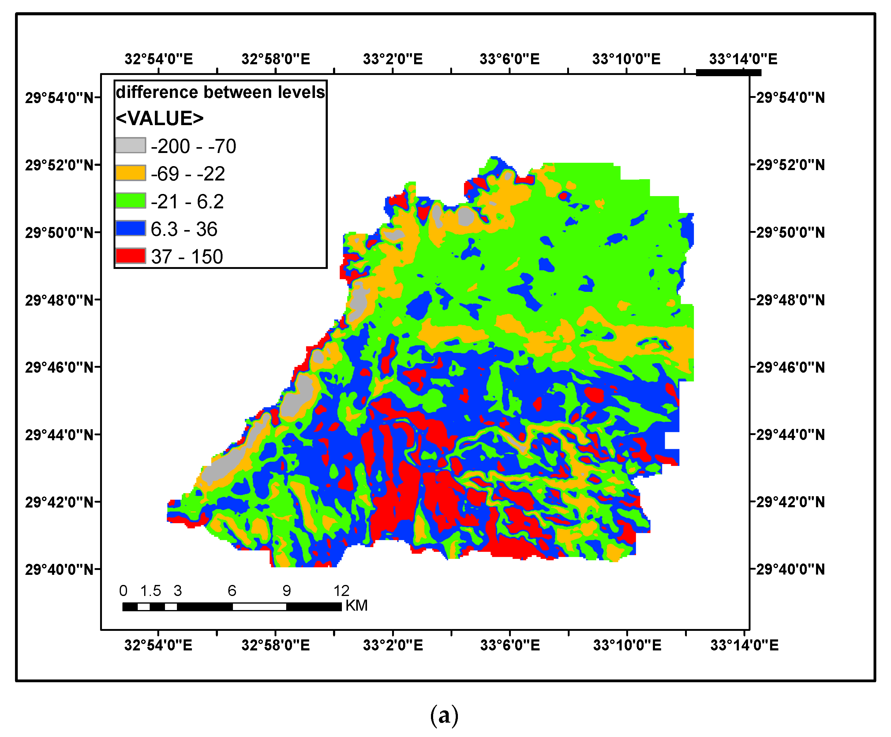
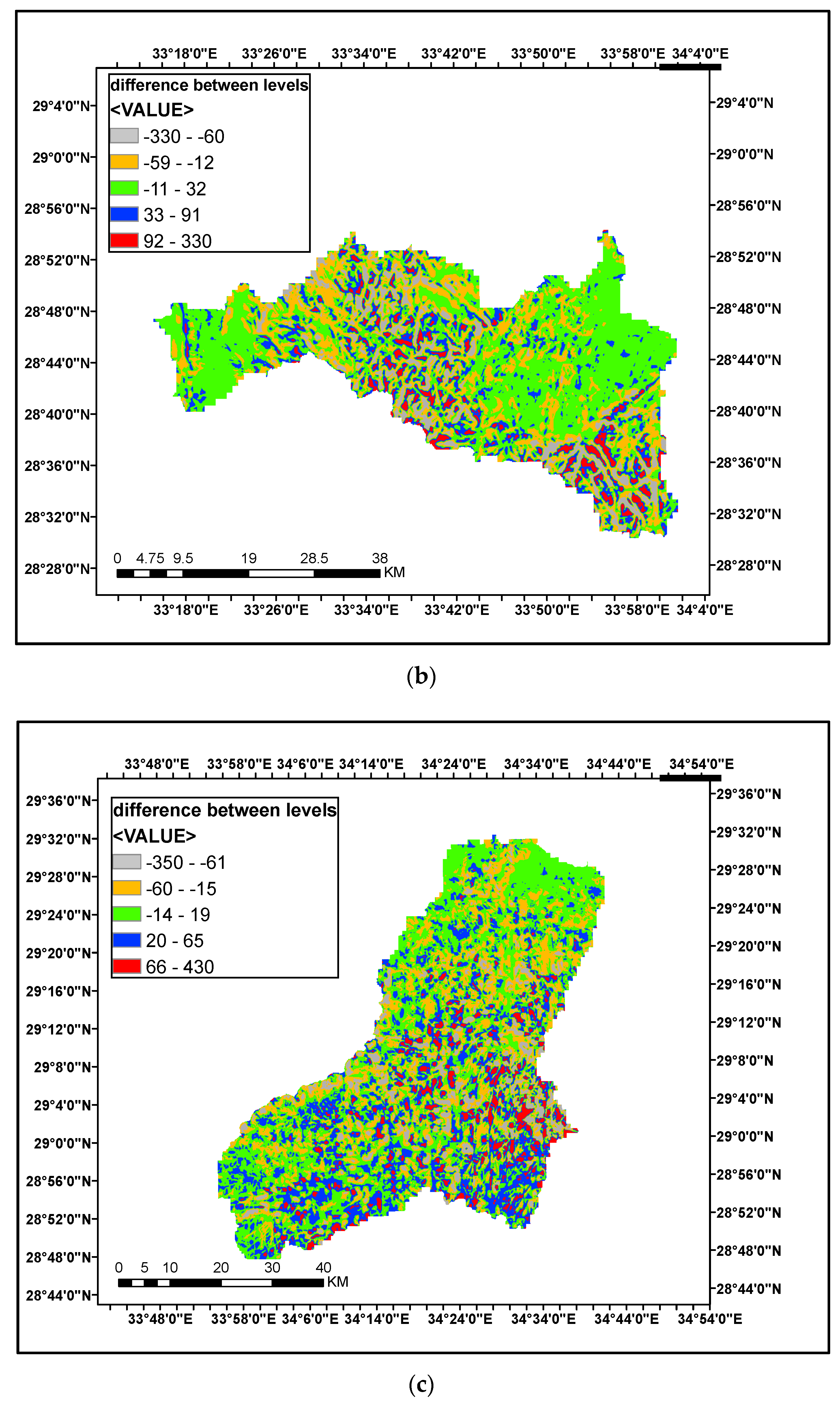
3. Results
4. Discussion
5. Conclusions
Author Contributions
Funding
Acknowledgments
Conflicts of Interest
References
- Jarvis, A.; Rubiano, J.; Nelson, A.; Farrow, A.; Mulligan, M. Practical Use of SRTM Data in the Tropics—Comparisons with Digital Elevation Models Generated from Cartographic Data; Working Document No. 198; Centro International de Agricultura Tropical (CIAT): Cali, Colombia, 2004. [Google Scholar]
- Farr, T.; Kobrick, M. The shuttle radar topography mission. Eos Trans. Am. Geophys. Union 2001, 82, 1–33. [Google Scholar] [CrossRef]
- Raaflaub, L.D.; Collins, M.J. The effect of error in gridded digital elevation models on the estimation of topographic parameters. Environ. Modell. Software 2006, 21, 710–732. [Google Scholar] [CrossRef]
- Mukherjee, S.; Garg, R.D.; Mukherjee, S. Effect of systematic error and its derived attributes: A case study on Dehradun area using Cartosat-1 stereo data. Indian J. Landsc. Syst. Ecol. Stud. 2011, 34, 45–58. [Google Scholar]
- Holmes, K.W.; Chadwick, O.A.; Kyriankidis, P.C. Error in USGS 30-m digital elevation model and its impact on terrain modelling. J. Hydrol. 2000, 233, 154–173. [Google Scholar] [CrossRef]
- Rabus, B.; Eineder, M.; Roth, A.; Bamler, R. The shuttle radar topography mission—A new class of digital elevation models acquired by space borne radar. ISPRS J. Photogramm. Remote Sens. 2003, 57, 241–262. [Google Scholar] [CrossRef]
- Rodriguez, E.; Morris, S.; Belz, E. A global assessment of the SRTM Performance. Photogramm. Eng. Remote Sens. 2006, 72, 249–260. [Google Scholar] [CrossRef]
- Kellndorfer, M.; Walker, S.; Pierce, E.; Dobson, C.; Fites, J.; Hunsaker, C. Vegetation height derivation from shuttle radar topography mission and national elevation data sets. Remote Sens. Environ. 2004, 93, 339–358. [Google Scholar] [CrossRef]
- Polidori, L.; El Hage, M.; Valeriano, M. Digital elevation model validation with no ground control: Application to the topodata DEM in Brazil. Bol. Ciênc. Geod. 2014, 20, 467–479. [Google Scholar] [CrossRef]
- Tachikawa, T.; Hato, M.; Kaku, M.; Iwasaki, A. Characteristics of ASTER GDEM version 2. In Proceedings of the 2011 IEEE International Geoscience and Remote Sensing Symposium, Vancouver, BC, Canada, 24–29 July 2011; pp. 3657–3660. [Google Scholar]
- Patel, A.; Katiyar, K.; Prasad, V. Performances evaluation of different open source DEM using Differential Global Positioning System (DGPS). Egypt. J. Remote Sens. Space Sci. 2016, 19, 7–16. [Google Scholar] [CrossRef] [Green Version]
- Wong, W.; Tsuyuki, S.; Ioki, K.; Phua, M. Accuracy assessment of global topographic data (SRTM & ASTER GDEM) in comparison with lidar for tropical montane forest. In Proceedings of the 35th Asian Conference on Remote Sensing, Nay Pyi Taw, Myanmar, 27–31 October 2014. [Google Scholar]
- Gesch, D.; Oimoen, M.; Zhang, Z.; Meyer, D.; Danielson, J. Validation of the aster global digital elevation model version 2 over the conterminous United States. In Proceedings of the ISPRS Congress, Melbourne, Australia, 25 August–1 September 2012. [Google Scholar]
- Thomas, J.; Joseph, S.; Thrivikramji, P.; Arunkumar, S. Sensitivity of digital elevation models: The scenario from two tropical mountain river basins of the Western Ghats, India. Geosci. Front. 2014, 5, 893–909. [Google Scholar] [CrossRef] [Green Version]
- Acharya, T.D.; Yang, I.T.; Lee, D.H. Comparative analysis of digital elevation models between AW3D30, SRTM30 and airborne LiDAR: A case of Chuncheon, South Korea. J. Korean Soc. Surv. Geod. Photogramm. Cartogr. 2018, 36, 17–24. [Google Scholar]
- Hector, A.; Cameron, A. Multi-scale relief model (MSRM): A new algorithm for the visualization of subtle topographic change of variable size in digital elevation models, earth surface processes and landforms. Earth Surf. Process. Landf. 2018, 43, 1361–1369. [Google Scholar]
- Alganci, U.; Besol, B.; Sertel, E. Accuracy assessment of different digital surface models. ISPRS Int. J. Geo Inf. 2018, 7, 114. [Google Scholar] [CrossRef]
- AQUAVEO. Watershed Modeling System WMS 8.1 Tutorials; Aquaveo: Provo, UT, USA, 2008; Available online: http://www.aquaveo.com/ (accessed on 15 June 2019).
- Blue-Marble-Geographics. Global Mapper User Manual, User Manual Book. Available online: Bluemarblegeo.com (accessed on 15 June 2019).
- Google Developers. Google Earth API Developer’s Guide, 2016; Google Developers: Mountain View, CA, USA, 2015. [Google Scholar]
- Water Resources Research Institute (WRRI). WRRI-Atlas Sainai Program; Version 1, Report; Water Resources Research Institute: Qanater, Egypt, 2012. [Google Scholar]


| Model | WMS | |
|---|---|---|
| General | Reference | Environmental Modeling Research Laboratory of Brigham Young University |
| Type | Watershed | |
| Scale | All sizes | |
| Interface | WINDOWS | |
| Inputs | Precipitation | Frequency storm, user-defined, hyetograph, gridded precipitation, SCS |
| Losses | Green-Ampt, SCS, gridded deficit constant, initial and constant | |
| Convert equations | Surface Runoff | Kinematic wave, SCS unit hydrograph, clark unit hydrograph, user-specified unit hydrograph and Snyder unit hydrograph |
| Output | Peak discharge and runoff hydrograph | |
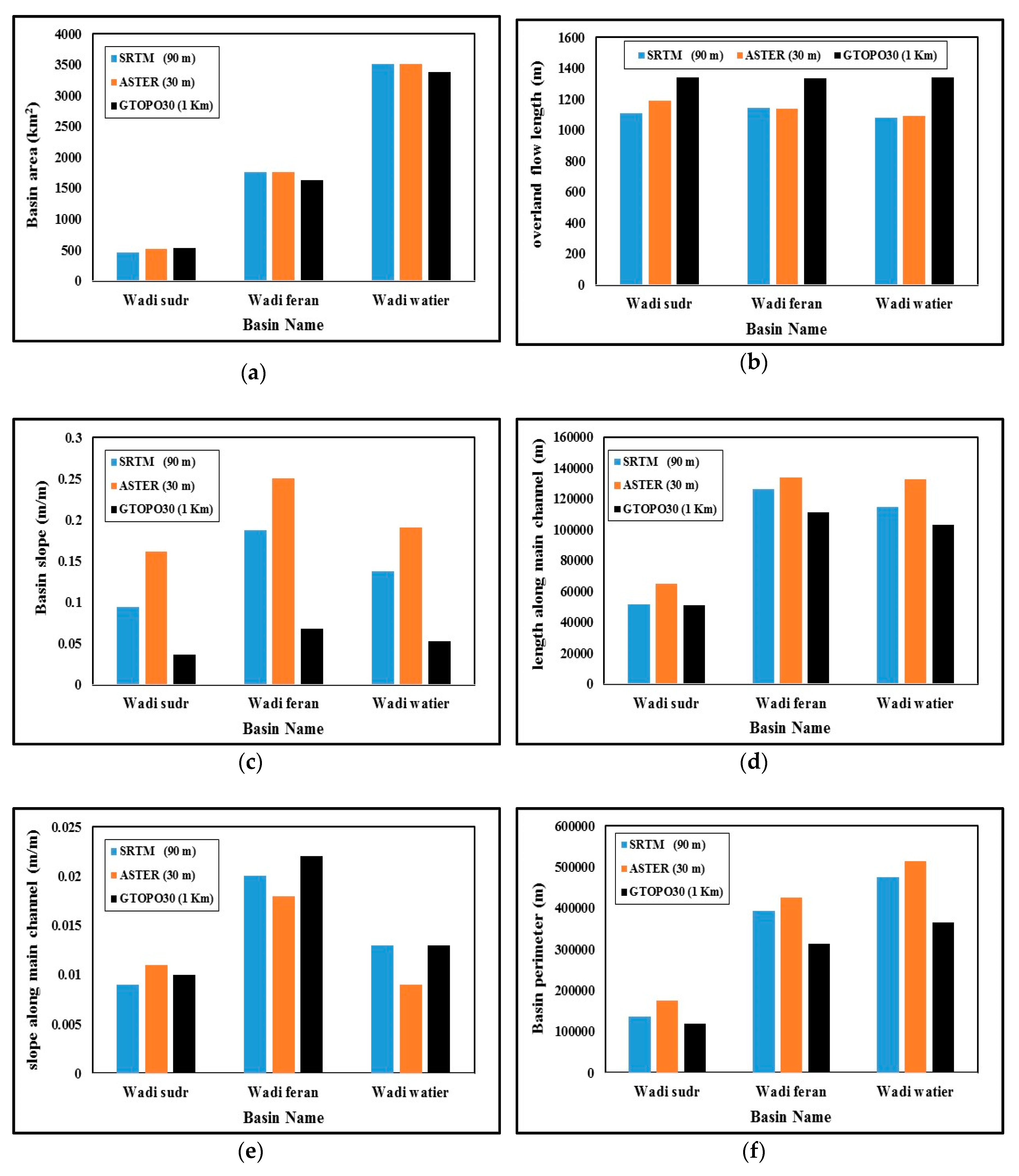
| Items | Wadi Sudr | Wadi Feran | Wadi Watier | ||||||
|---|---|---|---|---|---|---|---|---|---|
| SRTM (90 m) | ASTER (30 m) | GTOPO30 (1 Km) | SRTM (90 m) | ASTER (30 m) | GTOPO30 (1 Km) | SRTM (90 m) | ASTER (30 m) | GTOPO30 (1 Km) | |
| Basin area Km2 | 460 | 521 | 533 | 1767 | 1762 | 1631 | 3512 | 3517 | 3383 |
| Average overland flow length (m) | 1109 | 1189 | 1341 | 1143 | 1138 | 1336 | 1082 | 1094 | 1341 |
| Basin slope (m/m) | 0.094 | 0.161 | 0.036 | 0.187 | 0.250 | 0.068 | 0.137 | 0.191 | 0.053 |
| Basin length along main channel (m) | 51,499 | 64,673 | 50,973 | 126,529 | 133,607 | 111,439 | 114,460 | 132,760 | 103,180 |
| Basin slope along main channel (m/m) | 0.009 | 0.011 | 0.010 | 0.020 | 0.018 | 0.022 | 0.013 | 0.009 | 0.013 |
| Basin perimeter (m) | 137,100 | 176,110 | 119,580 | 394,350 | 426,170 | 314,430 | 475,600 | 515,060 | 365,060 |
| Shape factor | 2.43 | 2.72 | 2.11 | 3.24 | 3.26 | 3.46 | 1.51 | 1.51 | 1.50 |
© 2019 by the authors. Licensee MDPI, Basel, Switzerland. This article is an open access article distributed under the terms and conditions of the Creative Commons Attribution (CC BY) license (http://creativecommons.org/licenses/by/4.0/).
Share and Cite
Fathy, I.; Abd-Elhamid, H.; Zelenakova, M.; Kaposztasova, D. Effect of Topographic Data Accuracy on Watershed Management. Int. J. Environ. Res. Public Health 2019, 16, 4245. https://0-doi-org.brum.beds.ac.uk/10.3390/ijerph16214245
Fathy I, Abd-Elhamid H, Zelenakova M, Kaposztasova D. Effect of Topographic Data Accuracy on Watershed Management. International Journal of Environmental Research and Public Health. 2019; 16(21):4245. https://0-doi-org.brum.beds.ac.uk/10.3390/ijerph16214245
Chicago/Turabian StyleFathy, Ismail, Hany Abd-Elhamid, Martina Zelenakova, and Daniela Kaposztasova. 2019. "Effect of Topographic Data Accuracy on Watershed Management" International Journal of Environmental Research and Public Health 16, no. 21: 4245. https://0-doi-org.brum.beds.ac.uk/10.3390/ijerph16214245