Spatiotemporal Analysis and Control of Landscape Eco-Security at the Urban Fringe in Shrinking Resource Cities: A Case Study in Daqing, China

Abstract
:
1. Introduction
2. Materials and Methods
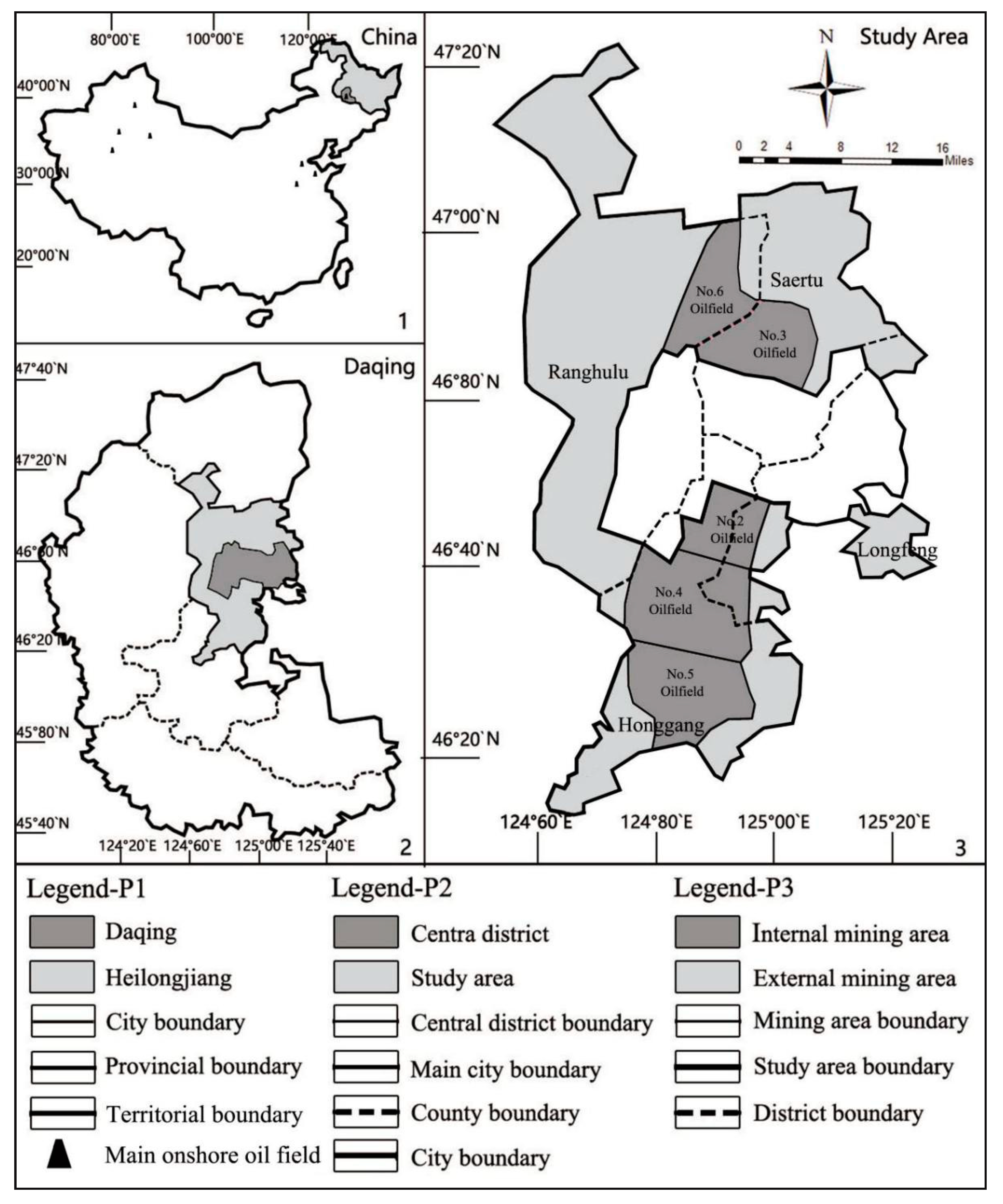
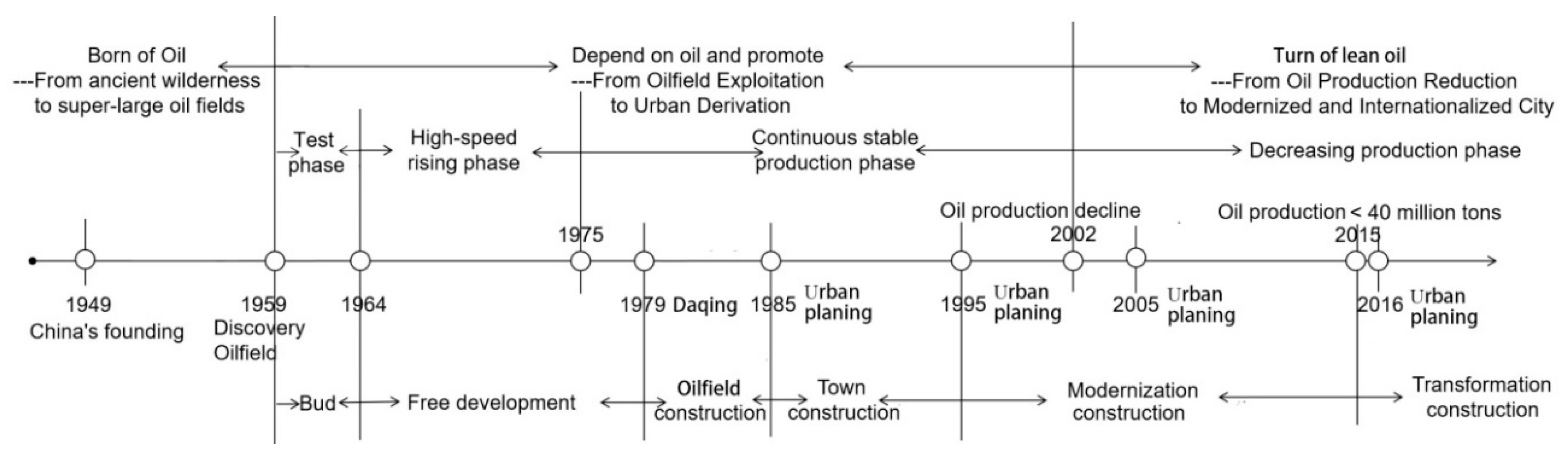
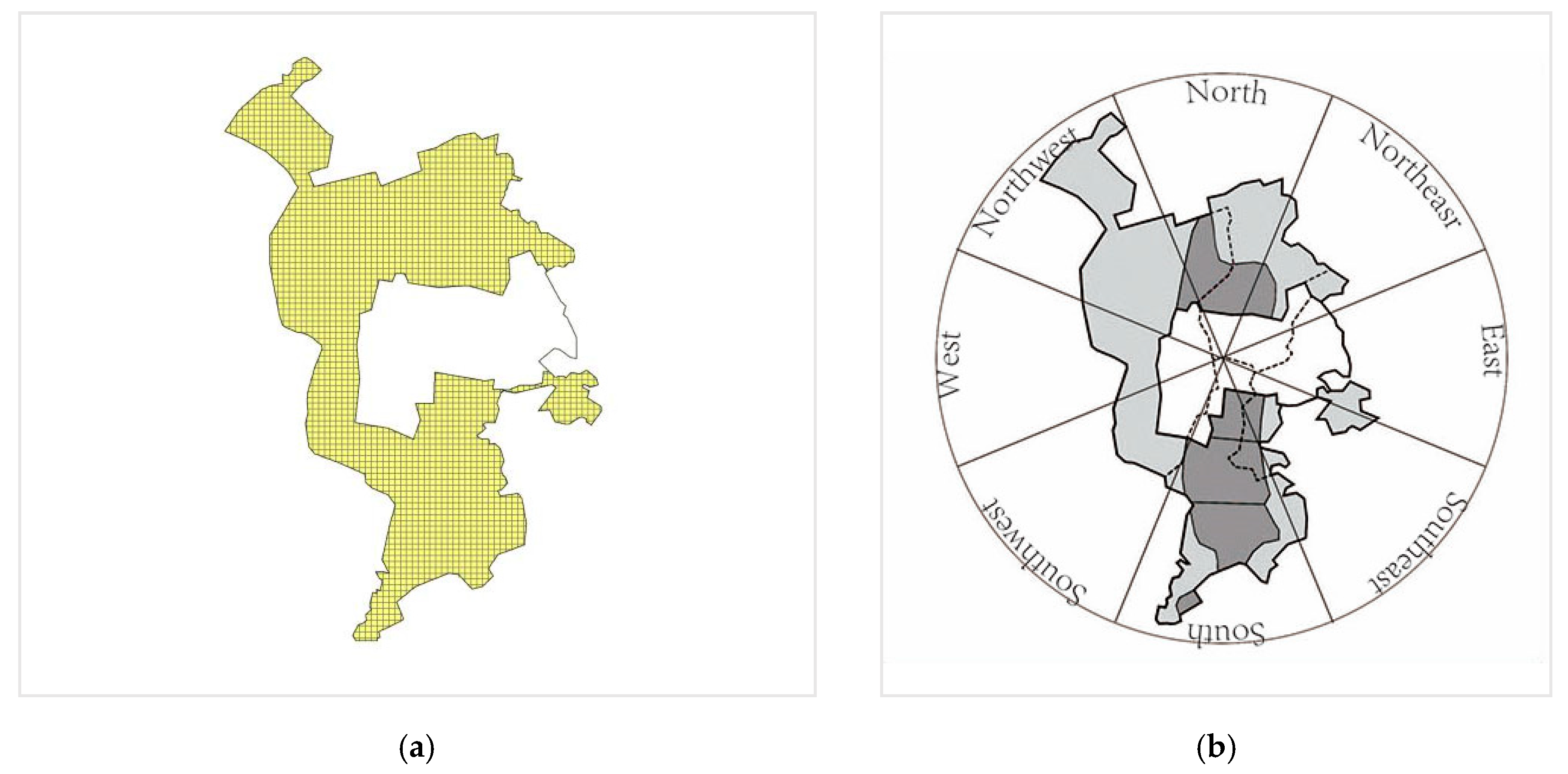
2.1. Study Area
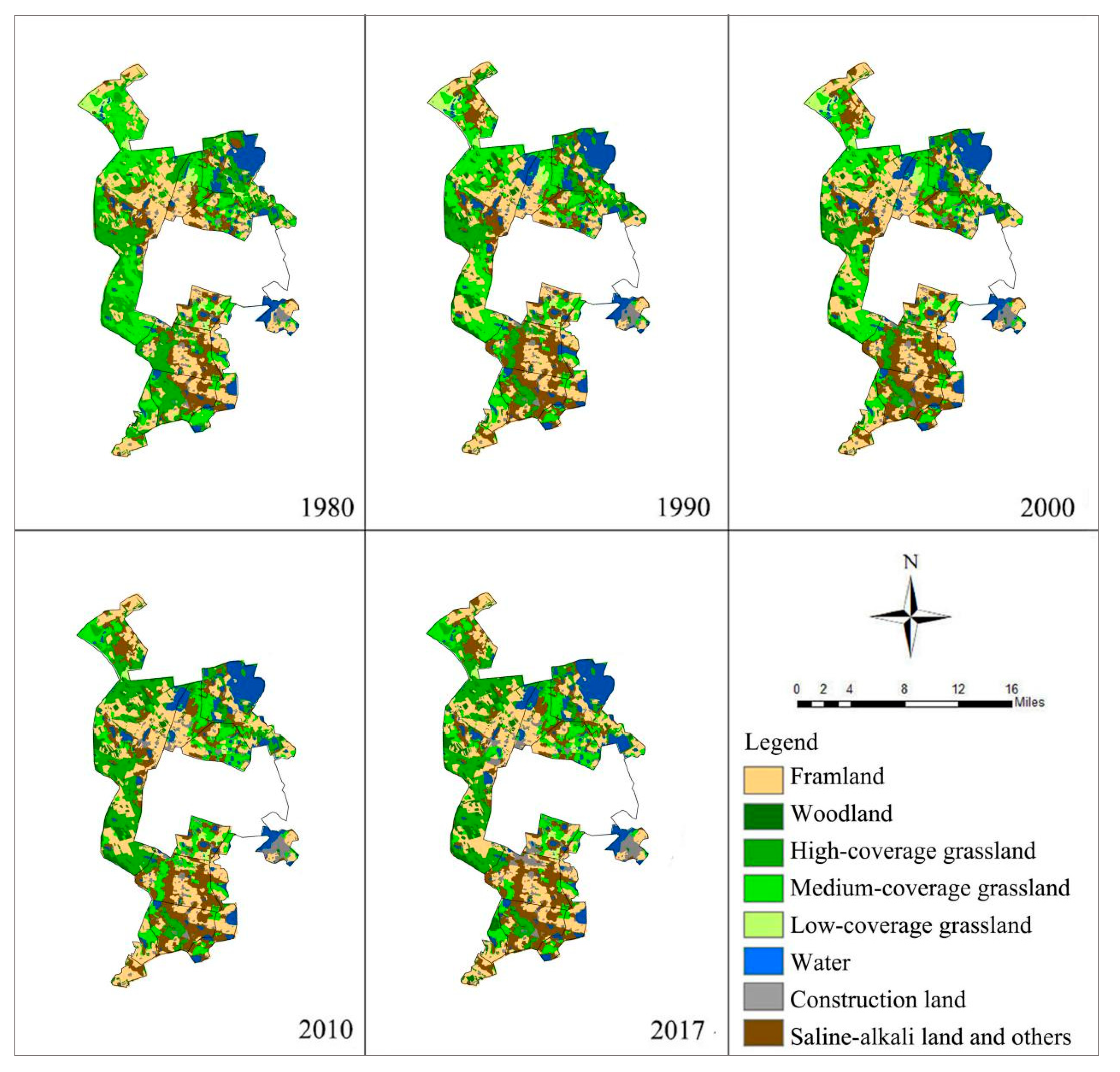
2.2. Data and Land Use Classification Criteria
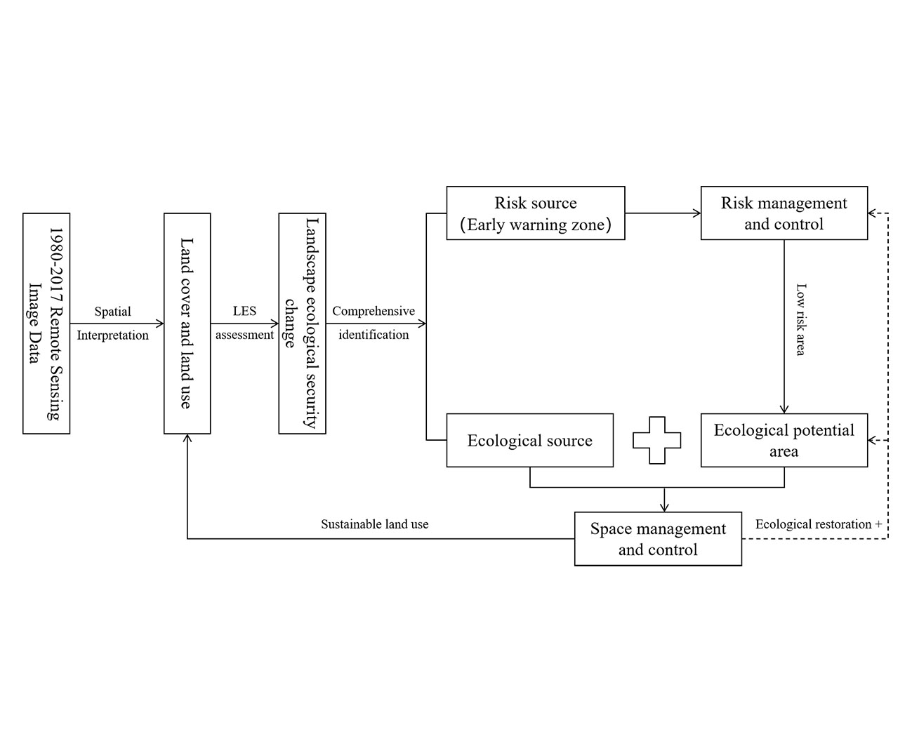
2.3. Methods
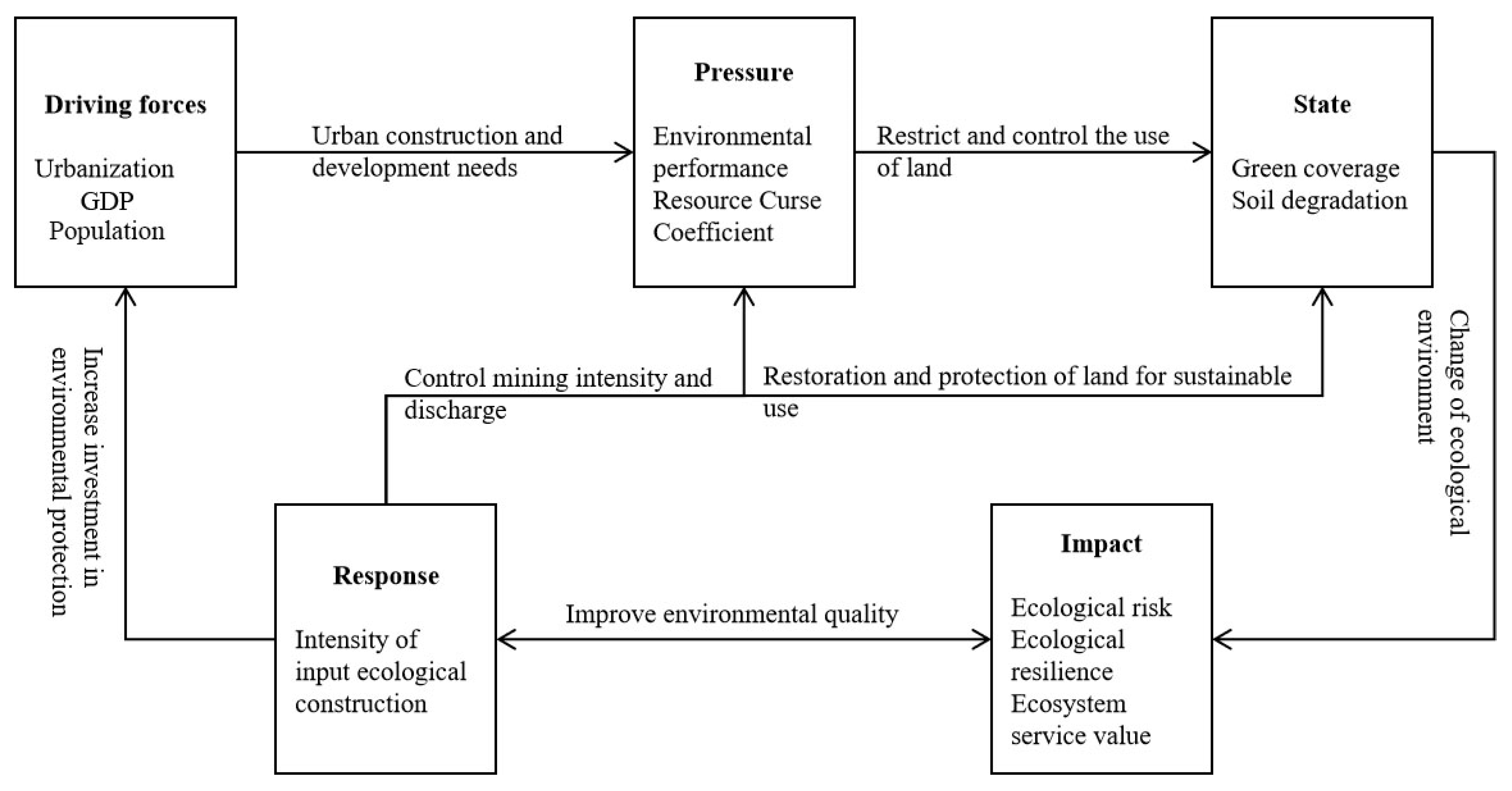
2.3.1. A Landscape Eco-Security Assessment System Based on the DPSIR Framework
2.3.2. Spatial Auto-Correlation Analysis
2.3.3. Space Partition Methods
3. Results
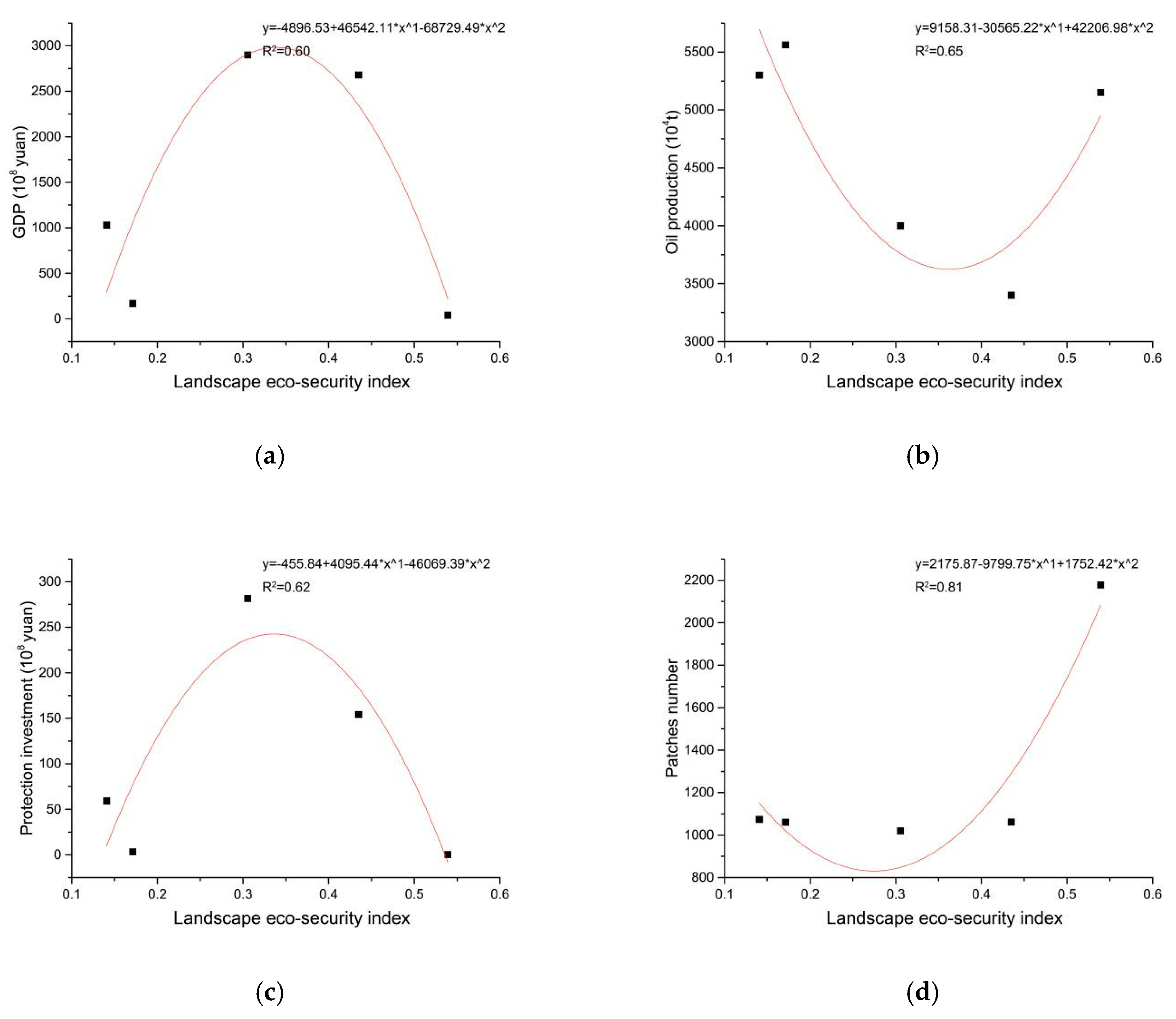
3.1. Trend of the Landscape Eco-Security Index
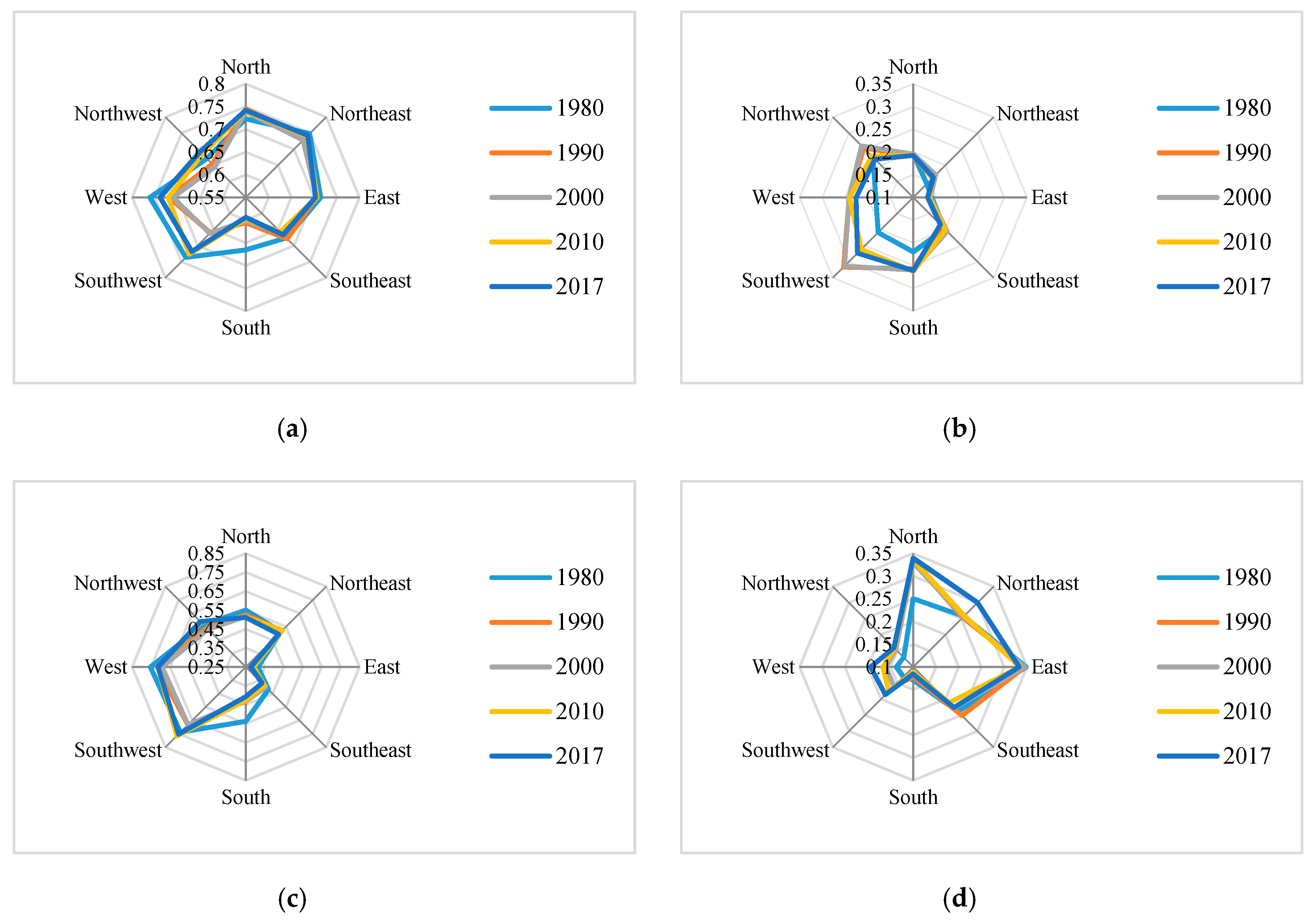
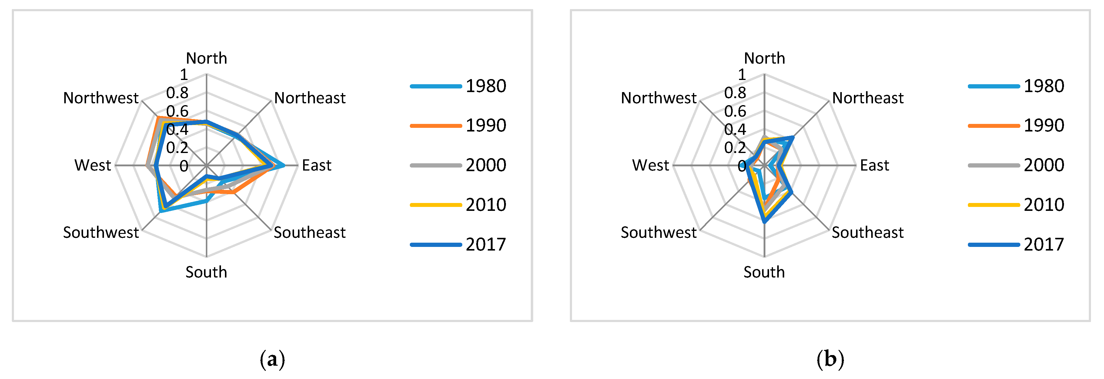
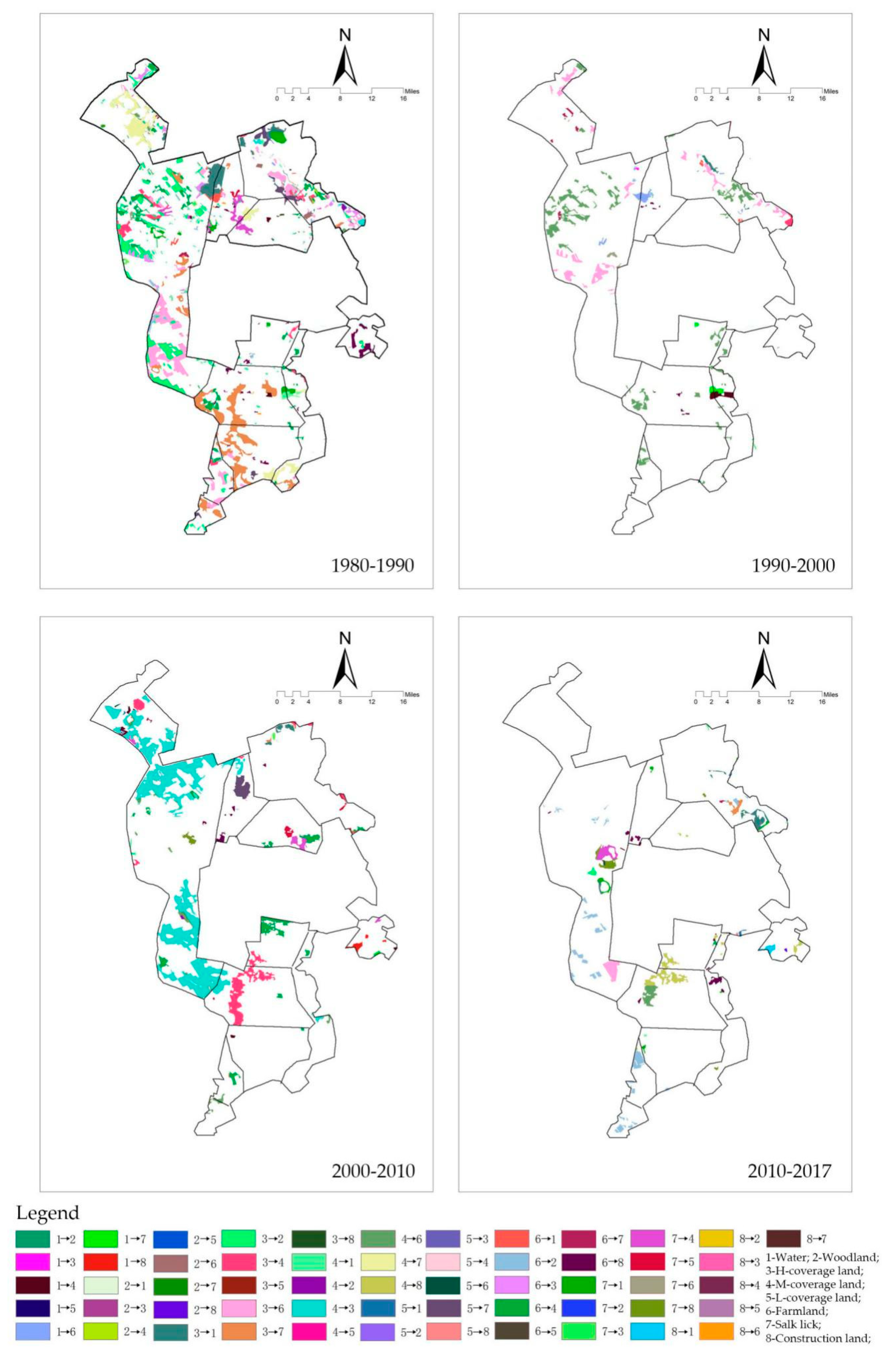
3.2. Spatial Auto-Correlation Trend
3.2.1. Global Auto-Correlation Analysis
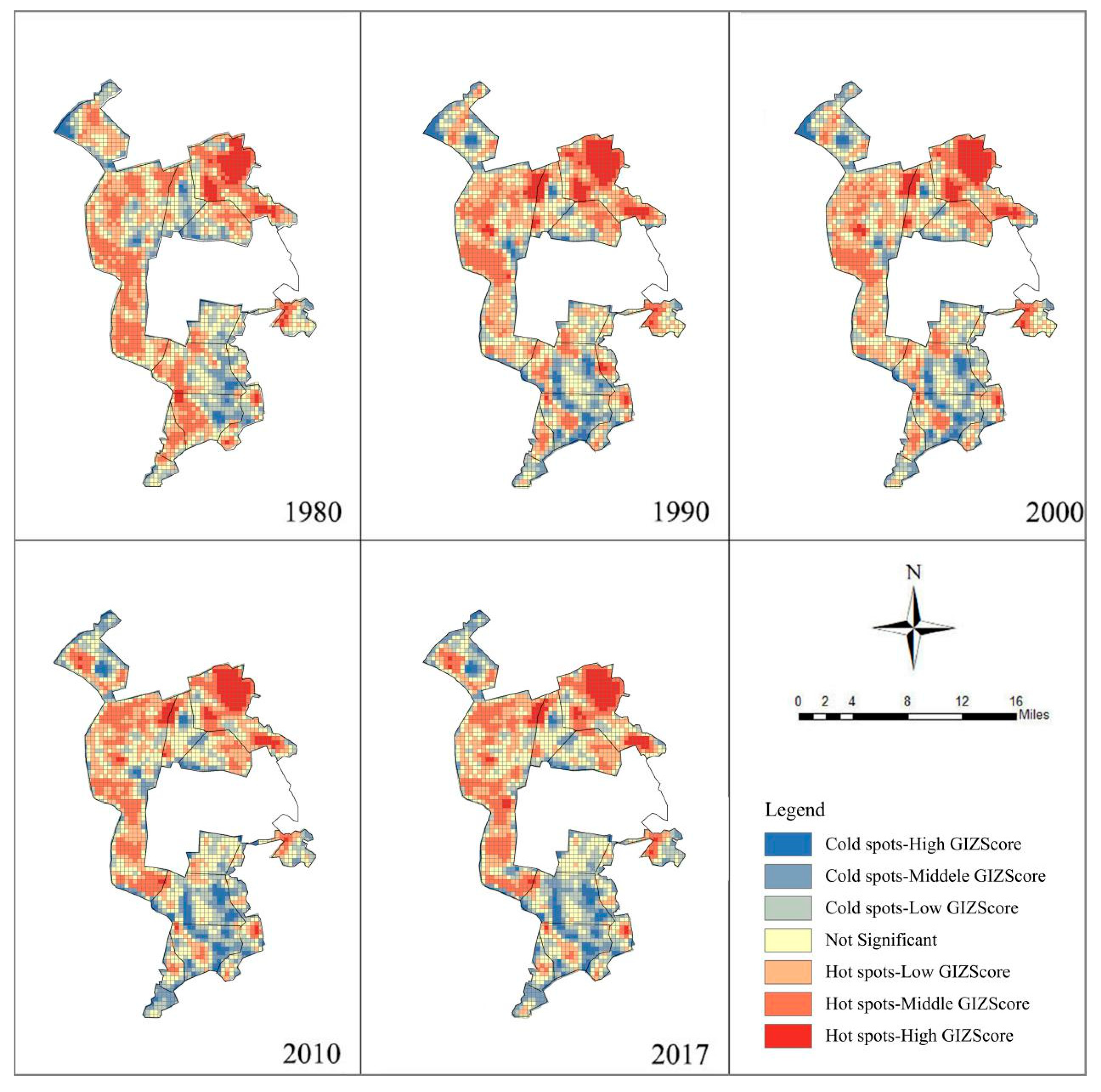
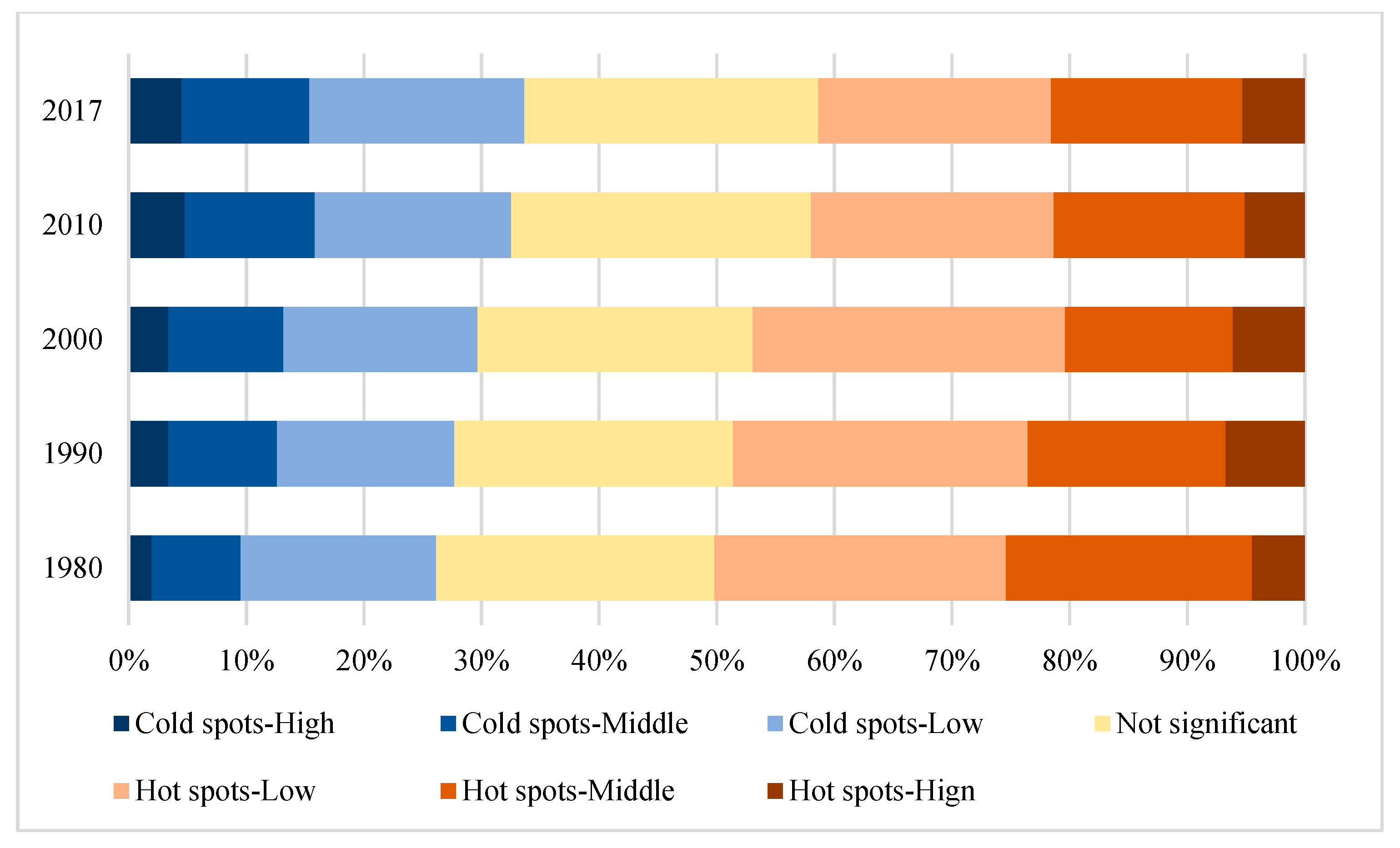
3.2.2. Local Spatial Autocorrelation Analysis
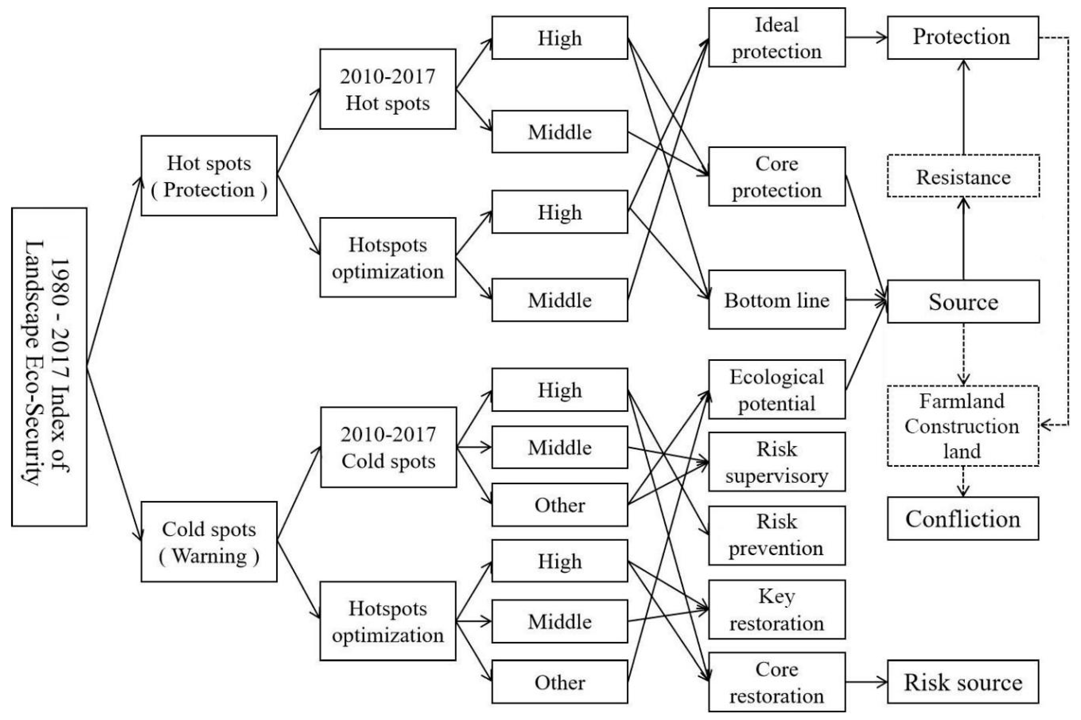
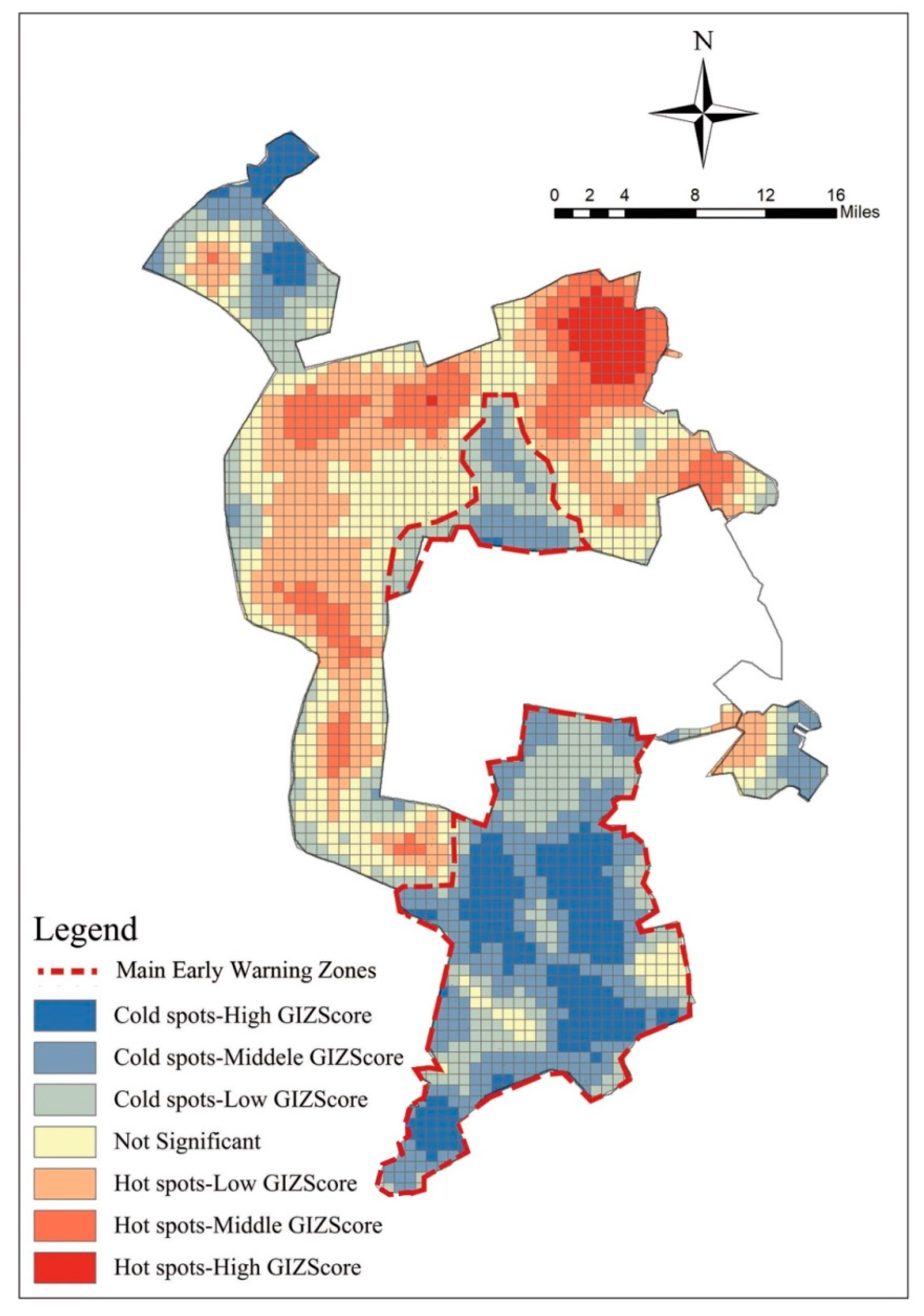
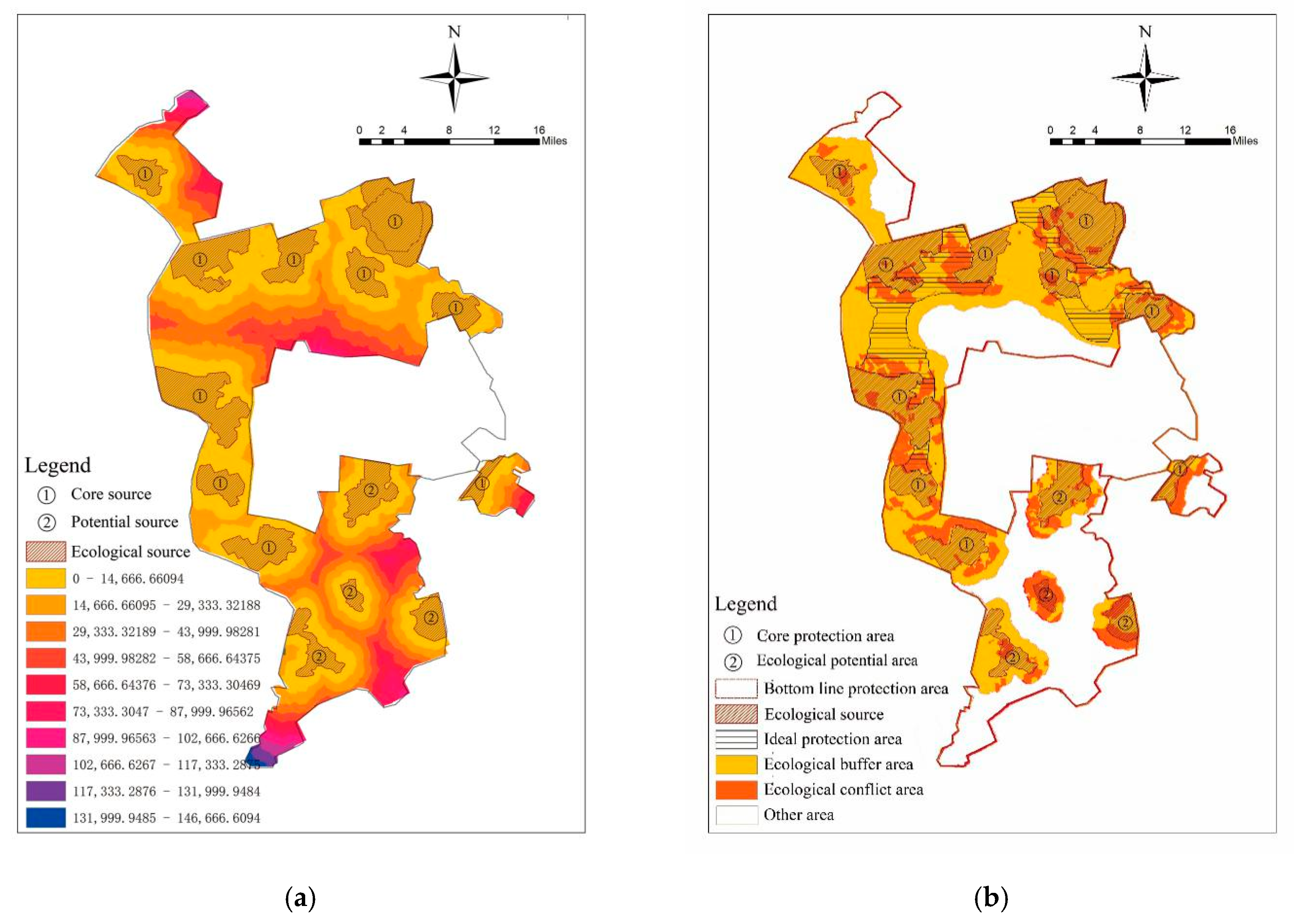
3.3. Space Partition
4. Discussion
4.1. The Main Reasons for Landscape Eco-Security Change
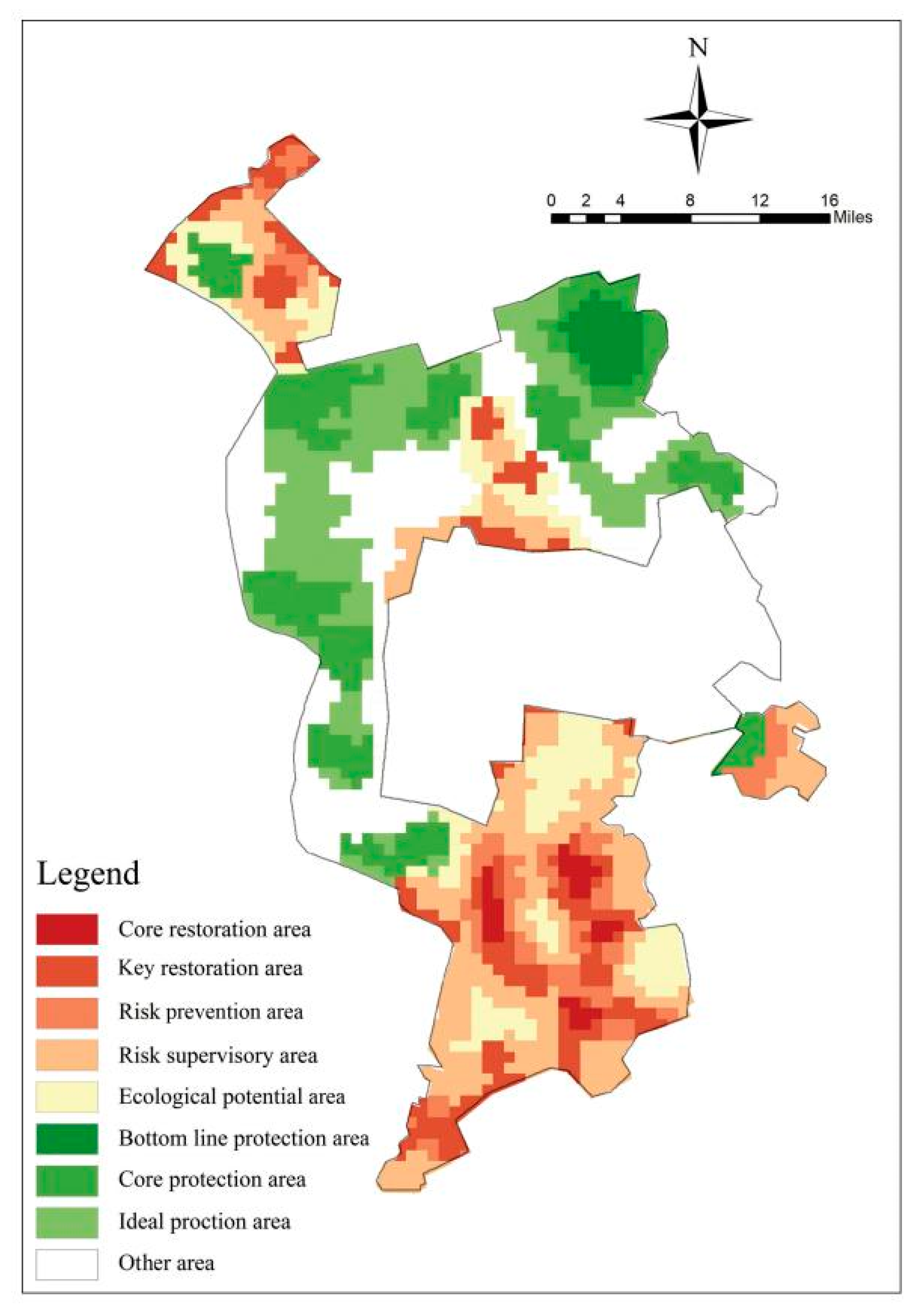
4.2. Risk Warning Area Control Strategies
4.3. Ecological Protection Area Control Strategies
5. Conclusions
Author Contributions
Funding
Acknowledgments
Conflicts of Interest
Appendix A

| Indicator | Formula | Parameter Meaning |
|---|---|---|
| Landscape Fragmentation Index (Ci) | Ni is the number of patches of landscape type i, A is the total area of the landscape (a plot) | |
| Landscape Separation Index (Ni) | Di is the distance index of landscape type i, Pi is the area index of landscape type i | |
| Landscape Dominance Index (Di) | DEi is the number of plaques in the unit type i/the total number of plaques in the unit, Pi is the area i in the unit/the total area of the unit | |
| Landscape Interference Index (Ei) | a, b, and c are the weights of each landscape index, and the three are added to 1. This paper assigns three indices to 0.502, 0.301, and 0.197 respectively. After calculating the Ci, Si, and DOi indicators according to the above formula, normalization is required due to different dimensions. | |
| Ecological Risk Loss Index (Ri) | Ei is the i-type land use interference index, Fi is the corresponding vulnerability index. |
| Land Use Type | Farmland | Woodland | High Coverage Grassland | Medium Coverage Grassland | Low Coverage Grassland | Water | Saline-Alkali Land | Construction Land |
|---|---|---|---|---|---|---|---|---|
| Level | 5 | 2 | 3 | 4 | 7 | 8 | 6 | 1 |
| Index | 0.8743 | 0.7048 | 0.7952 | 0.8440 | 0.9097 | 0.9208 | 0.8949 | 0.5 |
| Classification | Land Use Type | Score | Ecological Value |
|---|---|---|---|
| I (8–10) | Woodland | 9.0 | They have control and decisive significance in maintaining ecosystem elasticity. |
| High coverage grassland | 8.5 | ||
| II (6–8) | Medium coverage grassland | 7.0 | They play an important role in maintaining oasis stability and maintaining oasis regulation capacity, also can increase humidity and improve microbial cycle in local climate. |
| Farmland | 6.0 | ||
| III (2–4) | Water | 4.0 | It is necessary to strengthen management, effective maintenance, and careful use, if not well utilized, can easily reduce the elasticity of regional ecosystems. |
| Low coverage grassland | 2.0 | ||
| IV (0–2) | Saline-alkali land | 1.0 | They are the focus of ecological management and adjustment, but saline-alkali land is relatively stable, so the score is higher than desert. |
| Construction land | 0.0 |
| Land Use Type | Farmland | Woodland | High Coverage Grassland | Medium Coverage Grassland | Low Coverage Grassland | Water | Saline-Alkali Land | Construction Land |
|---|---|---|---|---|---|---|---|---|
| Equivalent factor | 8.76 | 21.19 | 7.02 | 5.36 | 3.75 | 52.67 | 0.83 | 0.41 |
| ESV (km2) | 7995.45 | 19,334.00 | 6406.81 | 4893.50 | 3424.56 | 48,067.77 | 761.01 | 371.66 |

References
- Galster, G. Why shrinking cities are not mirror images of growing cities: A research agenda of six testable propositions. Urban Aff. Rev. 2019, 55, 355–372. [Google Scholar] [CrossRef]
- Herrmann, D.; Shuster, W.; Mayer, A.; Garmestani, A.S. Sustainability for shrinking cities. Sustainability 2016, 8, 911. [Google Scholar] [CrossRef]
- Mabon, L.; Shih, W.Y. Management of sustainability transitions through planning in shrinking resource city contexts: An evaluation of Yubari City, Japan. J. Environ. Policy Plan. 2018, 20, 482–498. [Google Scholar] [CrossRef]
- McKinney, M.L.; Ingo, K.; Kendal, D. The contribution of wild urban ecosystems to liveable cities. Urban For. Urban Green. 2018, 29, 334–335. [Google Scholar] [CrossRef]
- Ibisch, P.L.; Hoffmann, M.T.; Kreft, S.; Pe’er, G.; Kati, V.; Biber-Freudenberger, L.; DellaSala, A.; Vale, M.M.; Hobson, P.R.; Selva, N. A global map of roadless areas and their conservation status. Science 2016, 354, 1423–1427. [Google Scholar] [CrossRef]
- Friedberger, M. The rural-urban fringe in the late twentieth century. Agric. Hist. 2000, 74, 502–514. [Google Scholar]
- Sullivan, W.C.; Lovell, S.T. Improving the visual quality of commercial development at the rural–urban fringe. Landsc. Urban Plan. 2006, 77, 152–166. [Google Scholar] [CrossRef]
- Yang, D.; Gao, X.; Xu, L.; Guo, Q. Constraint-adaptation challenges and resilience transitions of the industry–environmental system in a resource-dependent city. Resour. Conserv. Recycl. 2018, 134, 196–205. [Google Scholar] [CrossRef]
- Su, Y.; Chen, X.; Liao, J.; Zhang, H.; Wang, C.; Ye, Y.; Wang, Y. Modeling the optimal ecological security pattern for guiding the urban constructed land expansions. Urban For. Urban Green. 2016, 19, 35–46. [Google Scholar] [CrossRef]
- Chai, J.; Wang, Z.; Zhang, H. Integrated evaluation of coupling coordination for land use change and ecological security: A case study in Wuhan City of Hubei Province, China. Int. J. Environ. Res. Public Health 2017, 14, 1435. [Google Scholar] [CrossRef]
- Zhao, C.; Wang, C.; Yan, Y.; Shan, P.; Li, J.; Chen, J. Ecological security patterns assessment of Liao River Basin. Sustainability 2018, 10, 2401. [Google Scholar] [CrossRef]
- Hua, Y.E.; Yan, M.A.; Limin, D.O.N.G. Land ecological security assessment for Bai autonomous prefecture of Dali based using PSR model--with data in 2009 as case. Energy Procedia 2011, 5, 2172–2177. [Google Scholar] [CrossRef]
- Xu, J.; Fan, F.; Liu, Y.; Dong, J.; Chen, J. Construction of ecological security patterns in nature reserves based on ecosystem services and circuit theory: A case study in Wenchuan, China. Int. J. Environ. Res. Public Health 2019, 16, 3220. [Google Scholar] [CrossRef] [PubMed]
- Su, S.; Li, D.; Yu, X.; Zhang, Z.; Zhang, Q.; Xiao, R.; Zhi, J.; Wu, J. Assessing land ecological security in Shanghai (China) based on catastrophe theory. Stoch. Environ. Res. Risk Assess. 2011, 25, 737–746. [Google Scholar] [CrossRef]
- Xiaodan, W.; Xianghao, Z.; Pan, G. A GIS-based decision support system for regional eco-security assessment and its application on the Tibetan Plateau. J. Environ. Manag. 2010, 91, 1981–1990. [Google Scholar] [CrossRef]
- He, S.Y.; Lee, J.; Zhou, T.; Wu, D. Shrinking cities and resource-based economy: The economic restructuring in China’s mining cities. Cities 2017, 60, 75–83. [Google Scholar] [CrossRef]
- Hazeu, G.W.; Metzger, M.J.; Mücher, C.A.; Perez-Soba, M.; Renetzeder, C.H.; Andersen, E. European environmental stratifications and typologies: An overview. Agric. Ecosyst. Environ. 2011, 142, 29–39. [Google Scholar] [CrossRef]
- Gari, S.R.; Newton, A.; Icely, J.D. A review of the application and evolution of the DPSIR framework with an emphasis on coastal social-ecological systems. Ocean Coast. Manag. 2015, 103, 63–77. [Google Scholar] [CrossRef]
- Wang, Z.; Zhou, J.; Loaiciga, H.; Guo, H.; Hong, S. A DPSIR model for ecological security assessment through indicator screening: A case study at Dianchi Lake in China. PLoS ONE 2015, 10, e0131732. [Google Scholar] [CrossRef]
- Zhong, K.; Sun, C.; Ding, K. Study of ecological security changes in Dongjiang Watershed based on remote sensing. In Proceedings of the International Conference on Geo-Informatics in Resource Management and Sustainable Ecosystem, Wuhan, China, 8–10 November 2013; Springer: Berlin/Heidelberg, Germany, 2013; Volume 11, pp. 116–124. [Google Scholar] [CrossRef]
- Feng, Y.; Liu, Y.; Liu, Y. Spatially explicit assessment of land ecological security with spatial variables and logistic regression modeling in Shanghai, China. Stoch. Environ. Res. Risk Assess. 2017, 31, 2235–2249. [Google Scholar] [CrossRef]
- Gong, Z.; Wang, L. On consistency test method of expert opinion in ecological security assessment. Int. J. Environ. Res. Public Health 2017, 14, 1012. [Google Scholar] [CrossRef] [PubMed]
- Hu, M.; Li, Z.; Yuan, M.; Fan, C.; Xia, B. Spatial differentiation of ecological security and differentiated management of ecological conservation in the Pearl River Delta, China. Ecol. Indic. 2019, 104, 439–448. [Google Scholar] [CrossRef]
- McGarigal, K.; Compton, B.W.; Plunkett, E.B.; DeLuca, W.V.; Grand, J.; Ene, E.; Jackson, S.D. A landscape index of ecological integrity to inform landscape conservation. Landsc. Ecol. 2018, 33, 1029–1048. [Google Scholar] [CrossRef]
- Hong, W.; Jiang, R.; Yang, C.; Zhang, F.; Su, M.; Liao, Q. Establishing an ecological vulnerability assessment indicator system for spatial recognition and management of ecologically vulnerable areas in highly urbanized regions: A case study of Shenzhen, China. Ecol. Indic. 2016, 69, 540–547. [Google Scholar] [CrossRef]
- Li, F.; Ye, Y.; Song, B.; Wang, R. Evaluation of urban suitable ecological land based on the minimum cumulative resistance model: A case study from Changzhou, China. Ecol. Model. 2015, 318, 194–203. [Google Scholar] [CrossRef]
- Guo, R.; Wu, T.; Liu, M.; Huang, M.; Stendardo, L.; Zhang, Y. The construction and optimization of ecological security pattern in the Harbin-Changchun urban agglomeration, China. Int. J. Environ. Res. Public Health 2019, 16, 1190. [Google Scholar] [CrossRef]
- Wu, Z.; Lei, S.; He, B.J.; Bian, Z.; Wang, Y.; Lu, Q.; Peng, S.; Duo, L. Assessment of landscape ecological health: A case study of a mining city in a semi-arid steppe. Int. J. Environ. Res. Public Health 2019, 16, 752. [Google Scholar] [CrossRef]
- Wang, S.; Zhang, X.; Wu, T.; Yang, Y. The evolution of landscape ecological security in Beijing under the influence of different policies in recent decades. Sci. Total Environ. 2019, 646, 49–57. [Google Scholar] [CrossRef]
- Yang, J.; Guan, Y.; Xia, J.C.; Jin, C.; Li, X. Spatiotemporal variation characteristics of green space ecosystem service value at urban fringes: A case study on Ganjingzi District in Dalian, China. Sci. Total Environ. 2018, 639, 1453–1461. [Google Scholar] [CrossRef]
- Lu, C.; Wang, D.; Meng, P.; Yang, J.; Pang, M.; Wang, L. Research on resource curse effect of resource-dependent cities: Case study of Qingyang, Jinchang and Baiyin in China. Sustainability 2019, 11, 91. [Google Scholar] [CrossRef]
- Luo, F.; Liu, Y.; Peng, J.; Wu, J. Assessing urban landscape ecological risk through an adaptive cycle framework. Landsc. Urban Plan. 2018, 180, 125–134. [Google Scholar] [CrossRef]
- Mo, W.; Wang, Y.; Zhang, Y.; Zhuang, D. Impacts of road network expansion on landscape ecological risk in a megacity, China: A case study of Beijing. Sci. Total Environ. 2017, 574, 1000–1011. [Google Scholar] [CrossRef] [PubMed] [Green Version]
- Nguyen, A.K.; Liou, Y.A.; Li, M.H.; Tran, T.A. Zoning eco-environmental vulnerability for environmental management and protection. Ecol. Indic. 2016, 69, 100–117. [Google Scholar] [CrossRef]
- Cai, Y.; Zhang, Z.; Yan, J.; Gong, W.; Zhao, Q. Sea area grading methodology for coastal county-level administrative division in China: A case study. J. Coast. Res. 2019, 94 (Suppl. 1), 237–242. [Google Scholar] [CrossRef]
- Scherber, C.; Beduschi, T.; Tscharntke, T. Novel approaches to sampling pollinators in whole landscapes: A lesson for landscape-wide biodiversity monitoring. Landsc. Ecol. 2019, 34, 1057–1067. [Google Scholar] [CrossRef] [Green Version]
- Song, W.; Deng, X. Land-use/land-cover change and ecosystem service provision in China. Sci. Total Environ. 2017, 576, 705–719. [Google Scholar] [CrossRef]
- Wang, W.C.; Chang, Y.J.; Wang, H.C. An application of the spatial autocorrelation method on the change of real estate prices in Taitung City. ISPRS Int. J. Geo Inf. 2019, 8, 249. [Google Scholar] [CrossRef] [Green Version]
- Peng, J.; Pan, Y.; Liu, Y.; Zhao, H.; Wang, Y. Linking ecological degradation risk to identify ecological security patterns in a rapidly urbanizing landscape. Habitat Int. 2018, 71, 110–124. [Google Scholar] [CrossRef]
- Zhang, H.; Qi, Z.; Ye, X.; Cai, Y.; Ma, W.; Chen, M. Analysis of land use/land cover change, population shift, and their effects on spatiotemporal patterns of urban heat islands in metropolitan Shanghai, China. Appl. Geogr. 2013, 44, 121–133. [Google Scholar] [CrossRef]
- Akbar, T.A.; Hassan, Q.K.; Ishaq, S.; Batool, M.; Butt, H.J.; Jabbar, H. Investigative spatial distribution and modelling of existing and future urban land changes and its impact on urbanization and economy. Remote Sens. 2019, 11, 105. [Google Scholar] [CrossRef] [Green Version]
- Dewan, A.M.; Yamaguchi, Y.; Rahman, M.Z. Dynamics of land use/cover changes and the analysis of landscape fragmentation in Dhaka Metropolitan, Bangladesh. GeoJournal 2012, 77, 315–330. [Google Scholar] [CrossRef]
- Xu, L.; Chen, S.S.; Xu, Y.; Li, G.; Su, W. Impacts of land-use change on habitat quality during 1985–2015 in the Taihu Lake Basin. Sustainability 2019, 11, 3513. [Google Scholar] [CrossRef] [Green Version]
- Wang, S.; Chen, Y.; Wang, M.; Zhao, Y.; Li, J. SPA-based methods for the quantitative estimation of the soil salt content in saline-alkali land from field spectroscopy data: A case study from the Yellow River irrigation regions. Remote Sens. 2019, 11, 967. [Google Scholar] [CrossRef] [Green Version]
- Porrini, D.; Fusco, G.; Miglietta, P.P. Post-adversities recovery and profitability: The case of Italian farmers. Int. J. Environ. Res. Public Health 2019, 16, 3189. [Google Scholar] [CrossRef] [PubMed] [Green Version]
- Cai, H.; Yang, X.; Xu, X. Human-induced grassland degradation/restoration in the central Tibetan Plateau: The effects of ecological protection and restoration projects. Ecol. Eng. 2015, 83, 112–119. [Google Scholar] [CrossRef]
- Wang, H.; Takano, T.; Liu, S. Screening and evaluation of saline–alkaline tolerant germplasm of rice (Oryza sativa L.) in soda saline–alkali soil. Agronomy 2018, 8, 205. [Google Scholar] [CrossRef] [Green Version]
- Bai, Y.; Wong, C.P.; Jiang, B.; Hughes, A.C.; Wang, M.; Wang, Q. Developing China’s Ecological Redline Policy using ecosystem services assessments for land use planning. Nat. Commun. 2018, 9, 3034. [Google Scholar] [CrossRef] [Green Version]
- Hua, R.; Zhang, Y. Assessment of water quality improvements using the hydrodynamic simulation approach in regulated cascade reservoirs: A Case Study of drinking water sources of Shenzhen, China. Water 2017, 9, 825. [Google Scholar] [CrossRef] [Green Version]
- De Montis, A.; Caschili, S.; Mulas, M.; Modicad, G.; Ganciua, A.; Bardia, A.; Leddaa, A.; Dessenac, L.; Laudarid, L.; Ficherad, C.R. Urban–rural ecological networks for landscape planning. Land Use Policy 2016, 50, 312–327. [Google Scholar] [CrossRef]
- Li, J.; Qiu, R.; Li, K.; Xu, W. Informal land development on the urban fringe. Sustainability 2018, 10, 128. [Google Scholar] [CrossRef] [Green Version]
- Hong, W.; Yang, C.; Chen, L.; Zhang, F.; Shen, S.; Guo, R. Ecological control line: A decade of exploration and an innovative path of ecological land management for megacities in China. J. Environ. Manag. 2017, 191, 116–125. [Google Scholar] [CrossRef] [PubMed]


| Satellite | Date | Data Type | Band | Resolution | Cloud | Kappa |
|---|---|---|---|---|---|---|
| LANDSAT1–3 | 1980.07 | MSS | 4 | 30 M | 0 | 83.3% |
| LANDSAT4–5 | 1990.07 | TM | 7 | 30 M | 0 | 85.4% |
| LANDSAT7 | 2000.07 | ETM+ | 7 | 30 M | 0.01 | 86.8% |
| LANDSAT8 | 2010.07 | OLI–TIRS | 11 | 30 M | 0 | 87.1% |
| LANDSAT8 | 2017.07 | OLI–TIRS | 11 | 30 M | 0.01 | 87.8% |
| Name | Contents |
|---|---|
| Daqing Urban Planning | The boundary of the urban fringe; the specific content of the plan (especially in ecological environment construction) |
| Daqing Statistical Yearbook | Oilfield production; population; GDP; pollution consumption; the primary, secondary, and tertiary output value; environmental protection investment; population; |
| Daqing Oilfield Statistical Yearbook | Oilfield scope; oilfield ecological construction plan; |
| China Statistical Yearbook | GDP; mineral production (especially oilfield); pollution consumption; population; |
| Heilongjiang Agricultural Product Price Survey Yearbook | Planting area of grain crops in Daqing; total output value of grain crops in Daqing; |
| I | II | Description |
|---|---|---|
| Ecological land | Woodland | Forest land; shrub land; open forest land; |
| High coverage grassland | Grassland coverage >50%; | |
| Medium coverage grassland | Grassland coverage ranges from 20% to 50%; | |
| Low coverage grassland | Grassland coverage ranges from 5% to 20%; | |
| Water | Reservoirs; ponds; lakes; marshes; | |
| Non-ecological land | Farmland | Dry land; paddy field; |
| Construction land | Rural; Urban; industrial and transportation land; | |
| Saline-alkali land and others | Saline-alkali land; other unused land; |
| Dimension | Weight | Sub-Dimension | Indicator | Weight | (±) |
|---|---|---|---|---|---|
| D—Driving forces | 0.05 | Urbanization | D1—Urbanization growth intensity (UGI) | 0.5 | (+) |
| Economy; | D2—Per capita GDP | 0.5 | (+) | ||
| P—Pressure of landscape change | 0.2 | Oil production | P1—Resource Curse Coefficient (ESi) | 0.5 | (+) |
| Environment | P2—Environmental performance index (EPI) | 0.5 | (+) | ||
| S—State of land use | 0.2 | Ecological land | S1—Grassland degradation intensity (Ki1) | 0.25 | (−) |
| S2—Grassland restoration intensity (Ki2) | 0.25 | (+) | |||
| Non-ecological land | S3—Proportion of non-ecological land (Ui) | 0.5 | (−) | ||
| I—Impact of the landscape ecological system | 0.5 | Risk | I1—Ecological risk index (ERIk) | 0.5 | (−) |
| Resilience | I2—Ecological resilience (ECOres) | 0.25 | (+) | ||
| Service | I3—Ecosystem service value (ESV) | 0.25 | (+) | ||
| R—Human response | 0.05 | Human | R1—Intensity of input ecological construction (IEC) | 1 | (+) |
| Indicator | Equation | Description |
|---|---|---|
| D1 | Ubd is the urbanization index of the study city d in year-b, Uad is urbanization index of the study city d in year-a, Ub is the national urbanization index in year-b, and Ua is the national urbanization index in year-a. | |
| P1 | Ei is the resource production in region i, SIi is the output value of secondary industry in region i, and n is the number of regions. | |
| P2 | xi is the total consumption of urban i or pollutant i of the study city d; Xi is the total consumption of urban i or pollutant i in China; gd is the GDP of the study city d; and G is the national GDP. | |
| S1 | ΔSit1 is the area of grassland transferred to lower coverage grassland, construction land, saline–alkali land, and others. Sit is the area of grassland at the start of the study, and Δt is the time interval. | |
| S2 | ΔSit2 is the area of grassland transferred to higher coverage grassland, water, and woodland. Sit is the area of grassland at the start of the study, and Δt is the time interval. | |
| S3 | Si is the area of non-construction land. A is the total area of sampling block i. | |
| I1 | Aki is the area of land use type i in study area k, Ak is the area of study area k, Ei is the interference index of land use type i (Table A1), Fi is the vulnerability index of land use type i (Table A2), and n is the number of land use types. | |
| I2 | Ai is the area of land use type i in study area, Pi is the elastic score of land use type i, and n is the number of land use types. Ci is the landscape fragmentation index of land use type i (Table A3). | |
| I3 | Ai is the area of land use type i in study area, VCi is the total value coefficient of ecological function per unit area of land use type i (Table A4), and n is the number of land use types. | |
| R1 | EId is the amount of investment in ecological construction of the study city d, and gd is the GDP of the study city d. |
| Dimension | Weight | Indicator | Resistance Value |
|---|---|---|---|
| Land use | 0.5 | Water | 1 |
| Woodland | 2 | ||
| High coverage grassland | 3 | ||
| Medium coverage grassland | 4 | ||
| Low coverage grassland | 5 | ||
| Farmland | 6 | ||
| Saline–alkali land and others | 7 | ||
| Construction land | 8 | ||
| Overlying result | 0.5 | Core protection area (including Bottom line protection area) | 1 |
| Ecological potential area | 2 | ||
| Ideal protection area | 3 | ||
| Other area | 4 | ||
| Risk supervisory area | 5 | ||
| Risk prevention area | 6 | ||
| Key restoration area | 7 | ||
| Core restoration area | 8 |
| Global Auto-Correlation Index | 1980 | 1990 | 2000 | 2010 | 2017 |
|---|---|---|---|---|---|
| Moran’s Index | 0.473113 | 0.509808 | 0.493504 | 0.473886 | 0.502602 |
| Expected Index | −0.000427 | −0.000427 | −0.000427 | −0.000428 | −0.000428 |
| Variance | 0.000234 | 0.000241 | 0.000234 | 0.000235 | 0.000234 |
| Z-score | 30.932970 | 32.874252 | 32.260210 | 30.921220 | 32.884483 |
| P-value | 0.000000 | 0.000000 | 0.000000 | 0.000000 | 0.000000 |
| The Protection Area | Farmland | Construction Land | Development Proposals |
|---|---|---|---|
| Core protection area; Bottom line area | Returning farmland to a green–blue space | Dismantle | No construction, only for scientific research and education |
| Potential ecological area | Retain and convert to ecological farmland | Retain single-story ecological buildings | green infrastructures, such as ecological greenways, country parks, and country landscapes The ecological agriculture project, |
| Ideal protection area | Returning farmland to a green–blue space | Retain single-story ecological buildings | Construction of green infrastructures |
| Ecological buffer | Retain and convert to ecological farmland | Retain low-rise buildings | The ecological agriculture project; necessary rural living service facilities; cultivation production infrastructure; eco-tourism; leisure facilities |
© 2019 by the authors. Licensee MDPI, Basel, Switzerland. This article is an open access article distributed under the terms and conditions of the Creative Commons Attribution (CC BY) license (http://creativecommons.org/licenses/by/4.0/).
Share and Cite
Chen, X.; Xu, D.; Fadelelseed, S.; Li, L. Spatiotemporal Analysis and Control of Landscape Eco-Security at the Urban Fringe in Shrinking Resource Cities: A Case Study in Daqing, China. Int. J. Environ. Res. Public Health 2019, 16, 4640. https://0-doi-org.brum.beds.ac.uk/10.3390/ijerph16234640
Chen X, Xu D, Fadelelseed S, Li L. Spatiotemporal Analysis and Control of Landscape Eco-Security at the Urban Fringe in Shrinking Resource Cities: A Case Study in Daqing, China. International Journal of Environmental Research and Public Health. 2019; 16(23):4640. https://0-doi-org.brum.beds.ac.uk/10.3390/ijerph16234640
Chicago/Turabian StyleChen, Xi, Dawei Xu, Safa Fadelelseed, and Lianying Li. 2019. "Spatiotemporal Analysis and Control of Landscape Eco-Security at the Urban Fringe in Shrinking Resource Cities: A Case Study in Daqing, China" International Journal of Environmental Research and Public Health 16, no. 23: 4640. https://0-doi-org.brum.beds.ac.uk/10.3390/ijerph16234640