Flow Dynamics and Contaminant Transport in Y-Shaped River Channel Confluences

Abstract
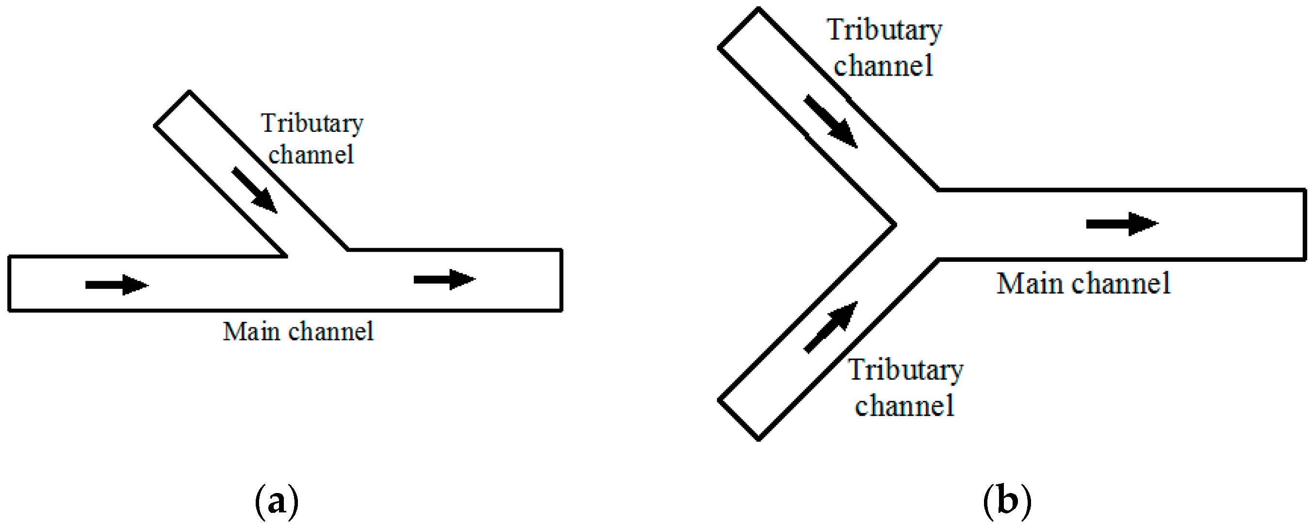
:1. Introduction
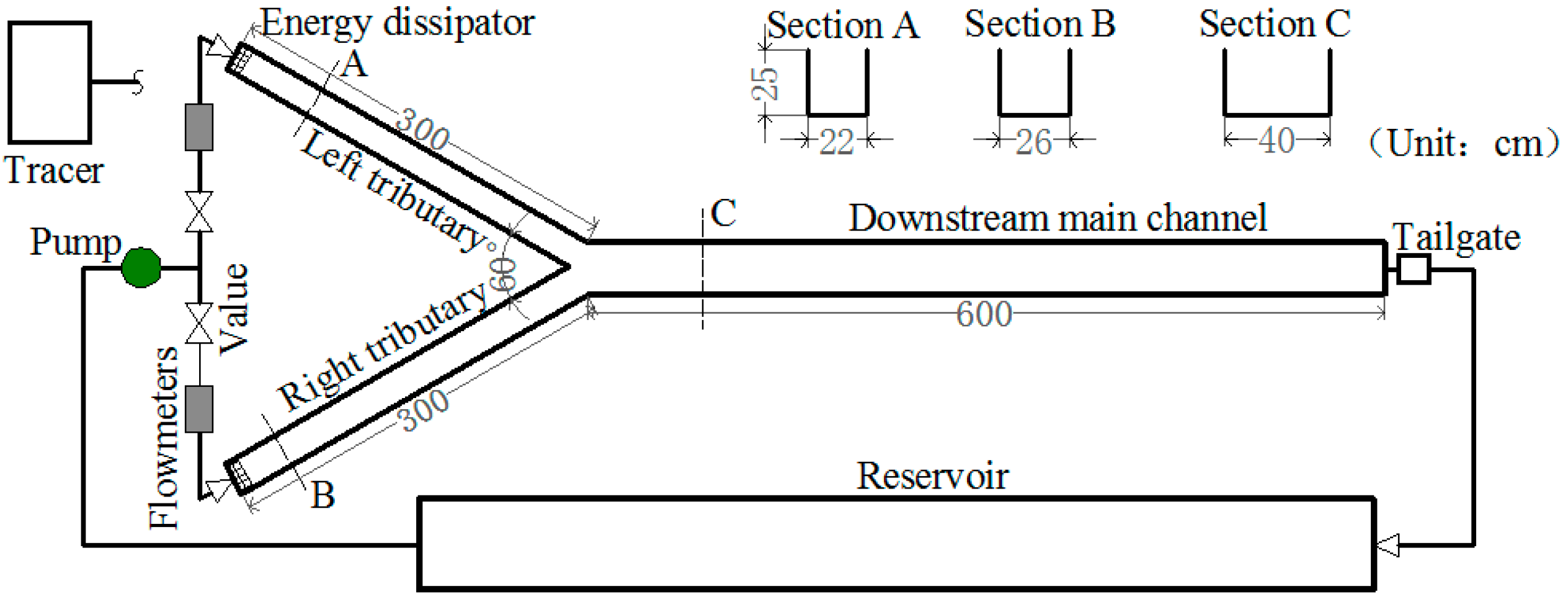
2. Materials and Methods
3. Results and Discussion
3.1. Flow Dynamics at Channel Confluences Transport of Contaminants at Channel Confluences
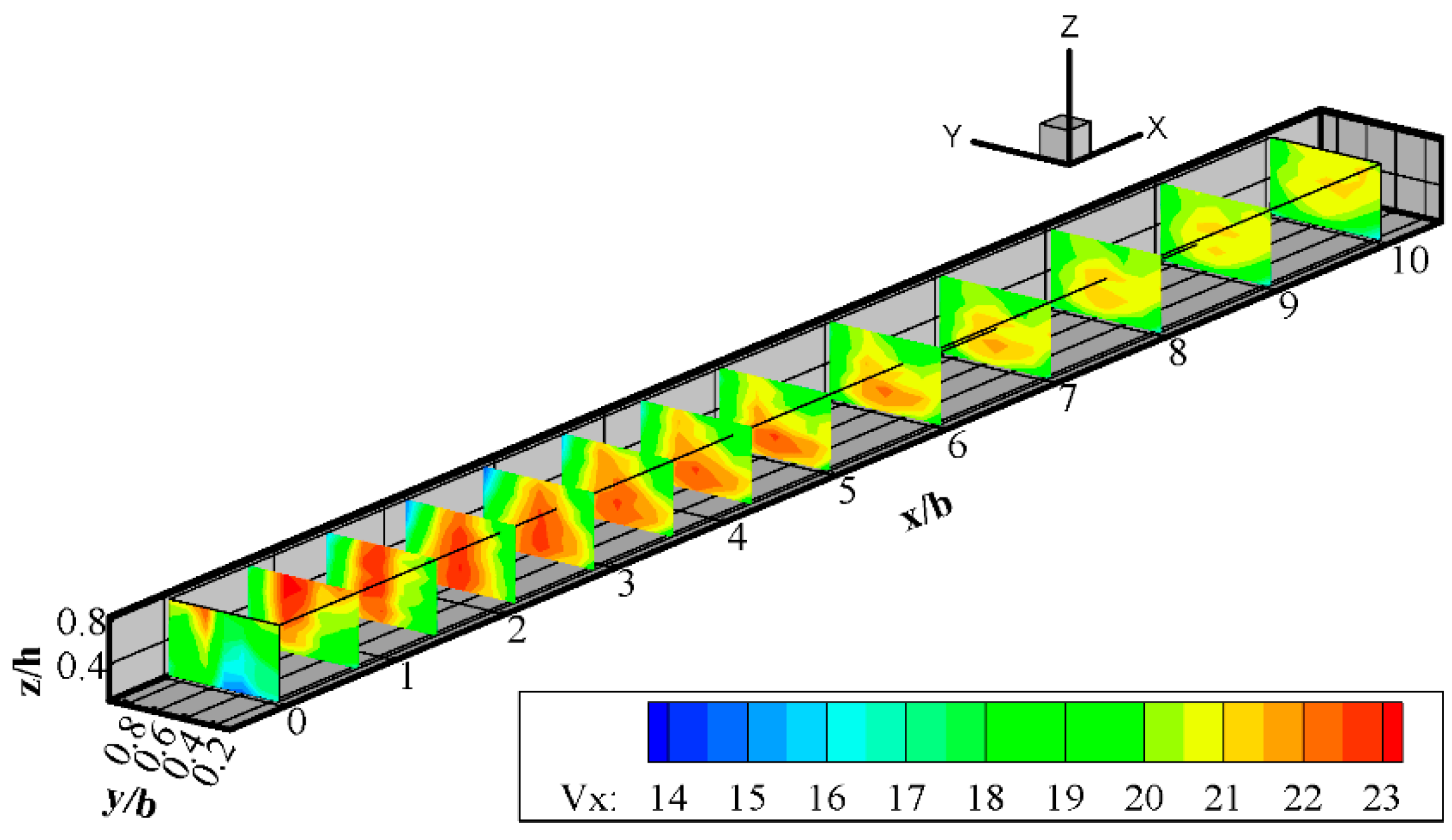
3.1.1. Longitudinal Velocity
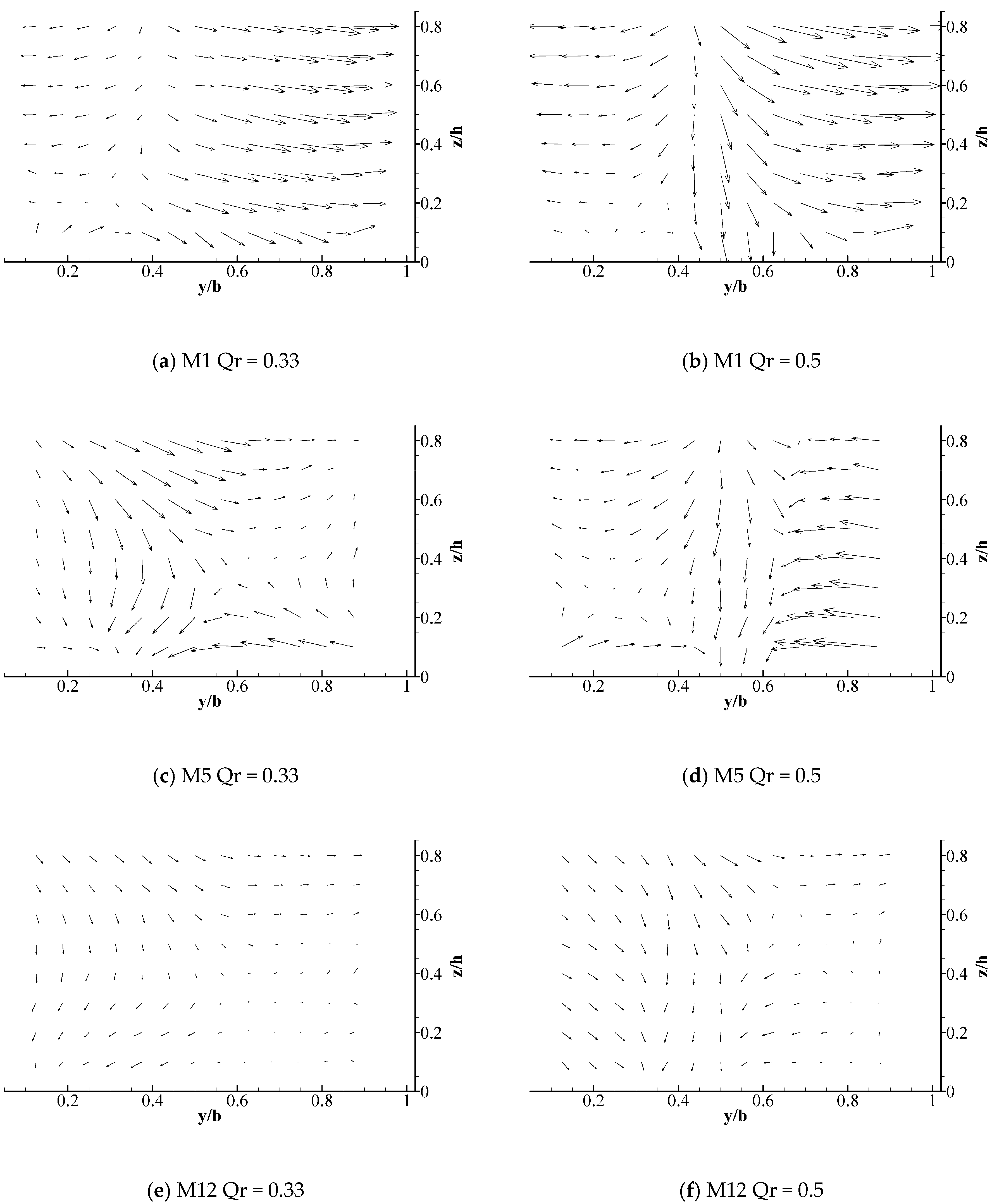
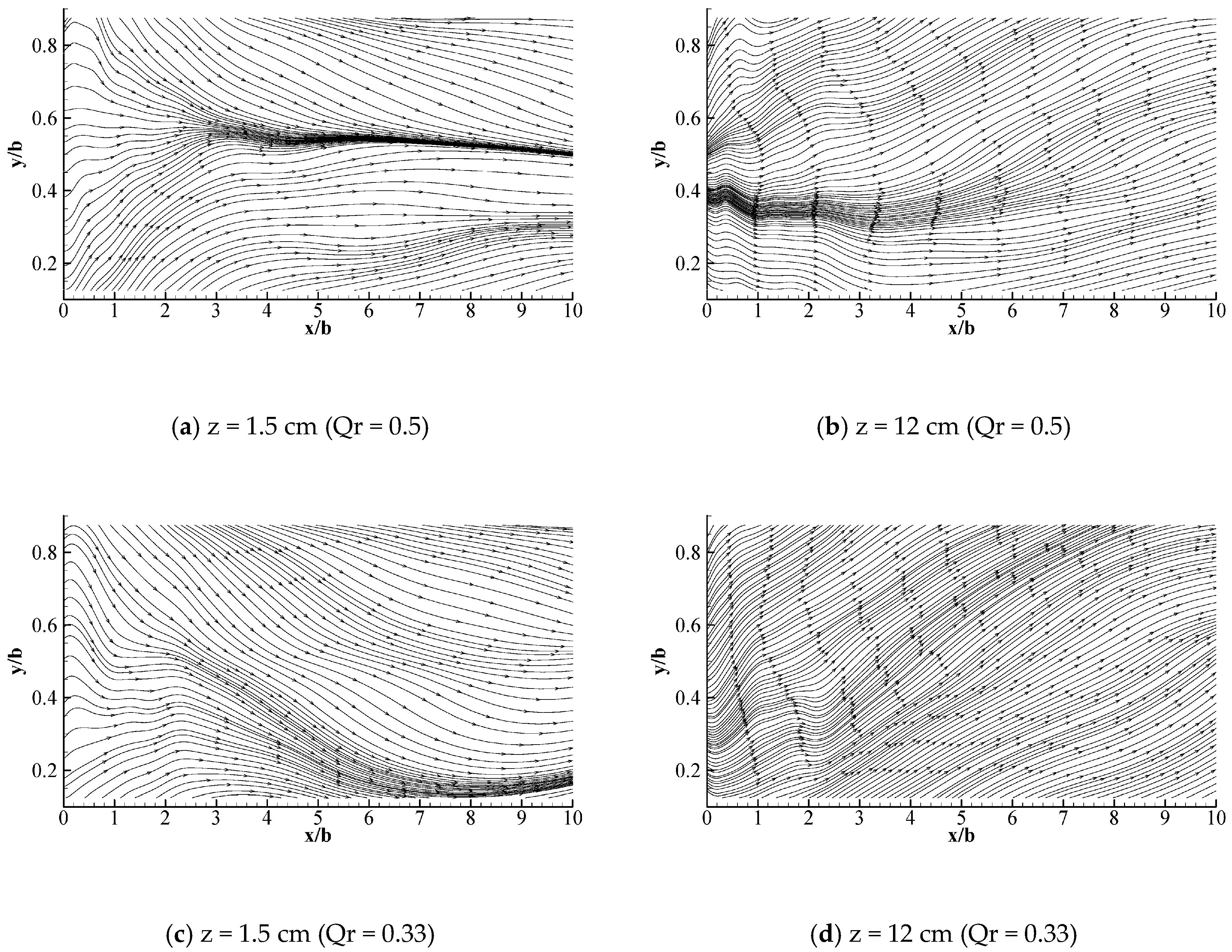
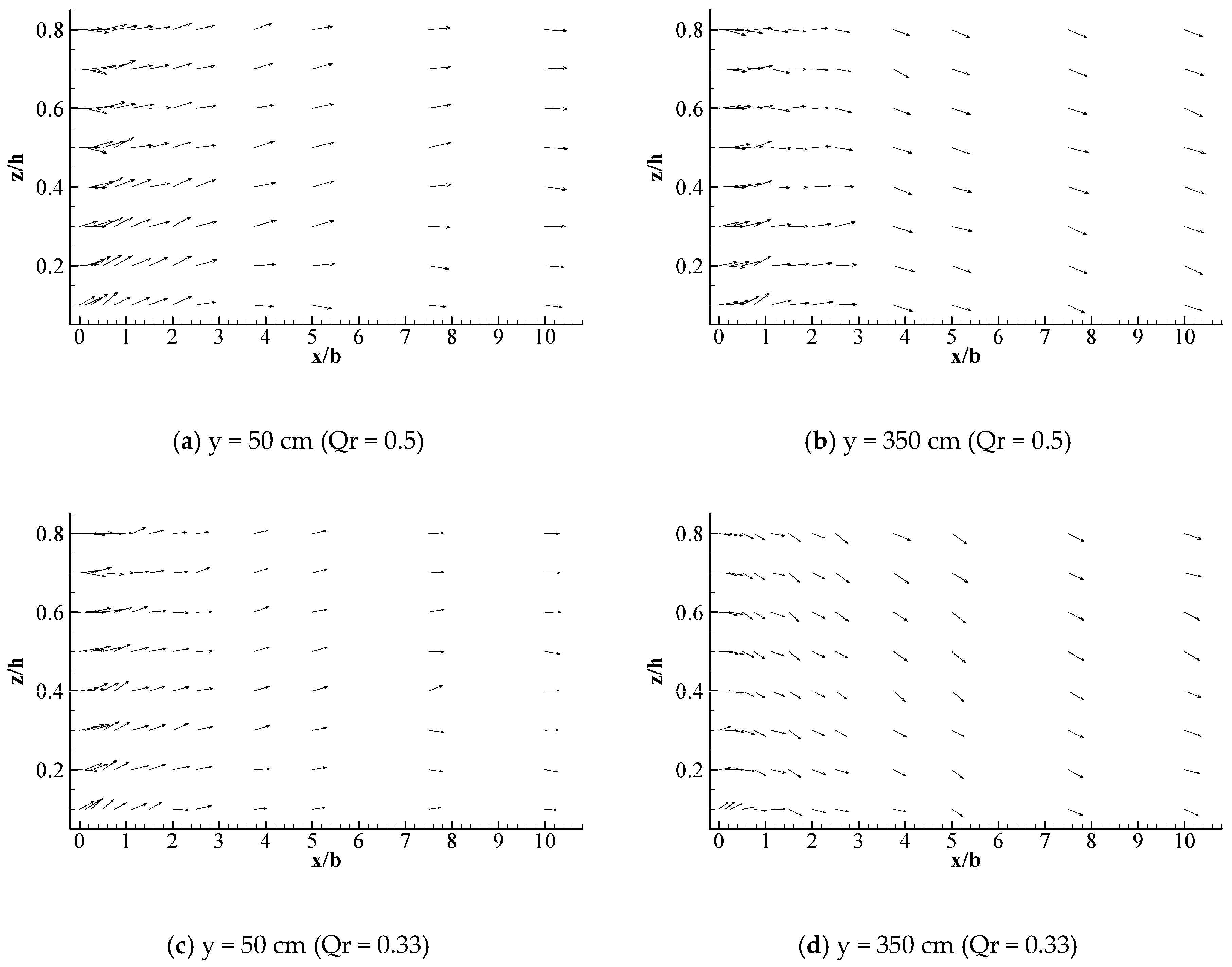
3.1.2. Secondary Current and Two Helical Cells
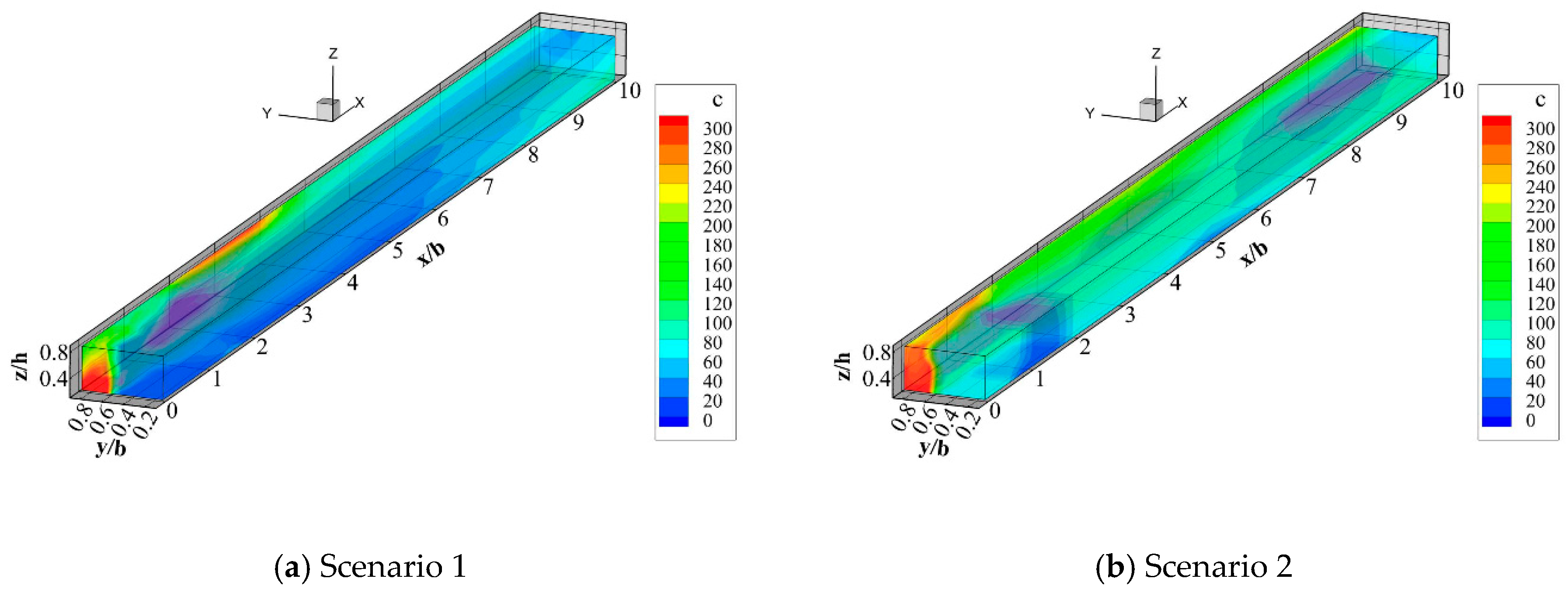
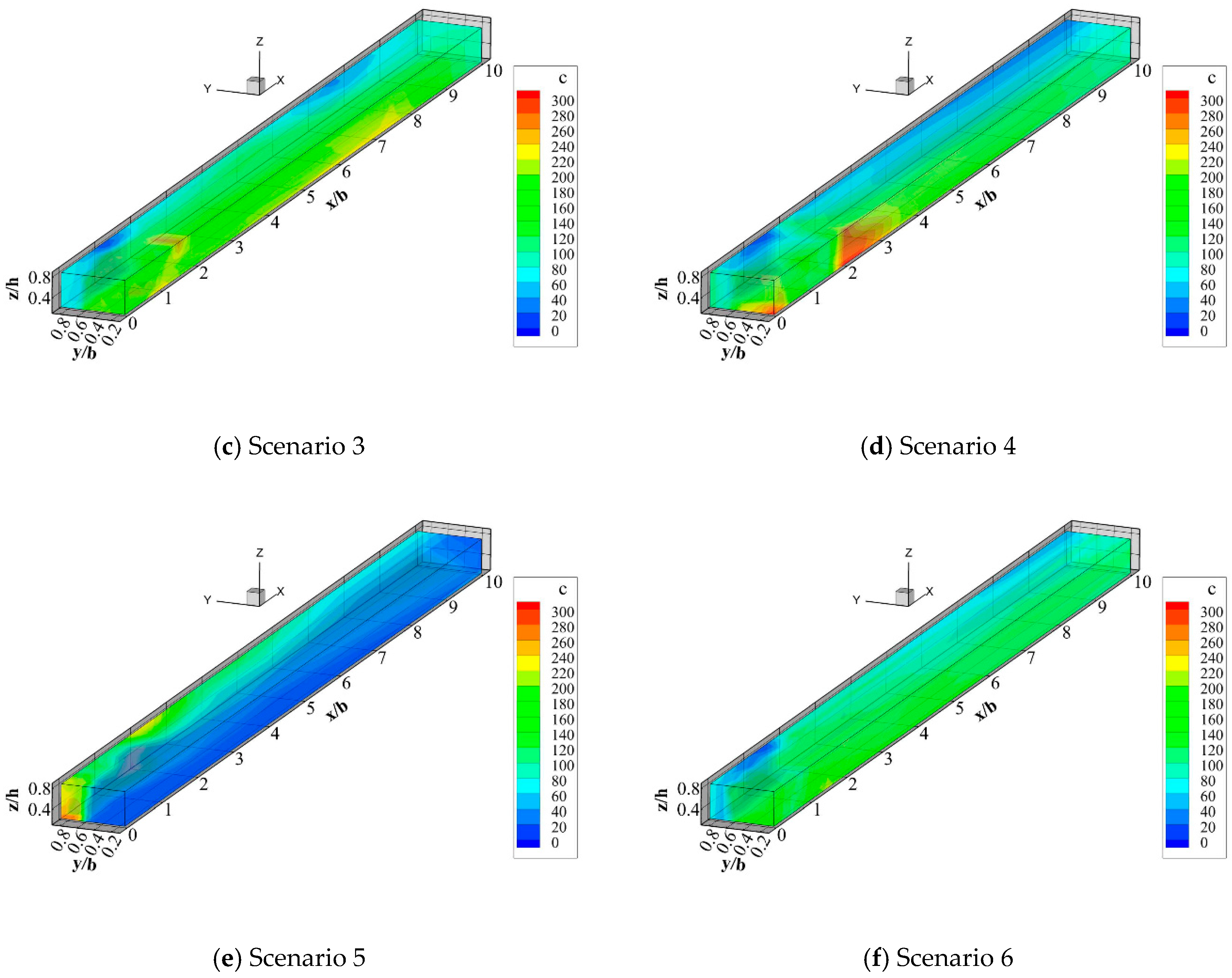
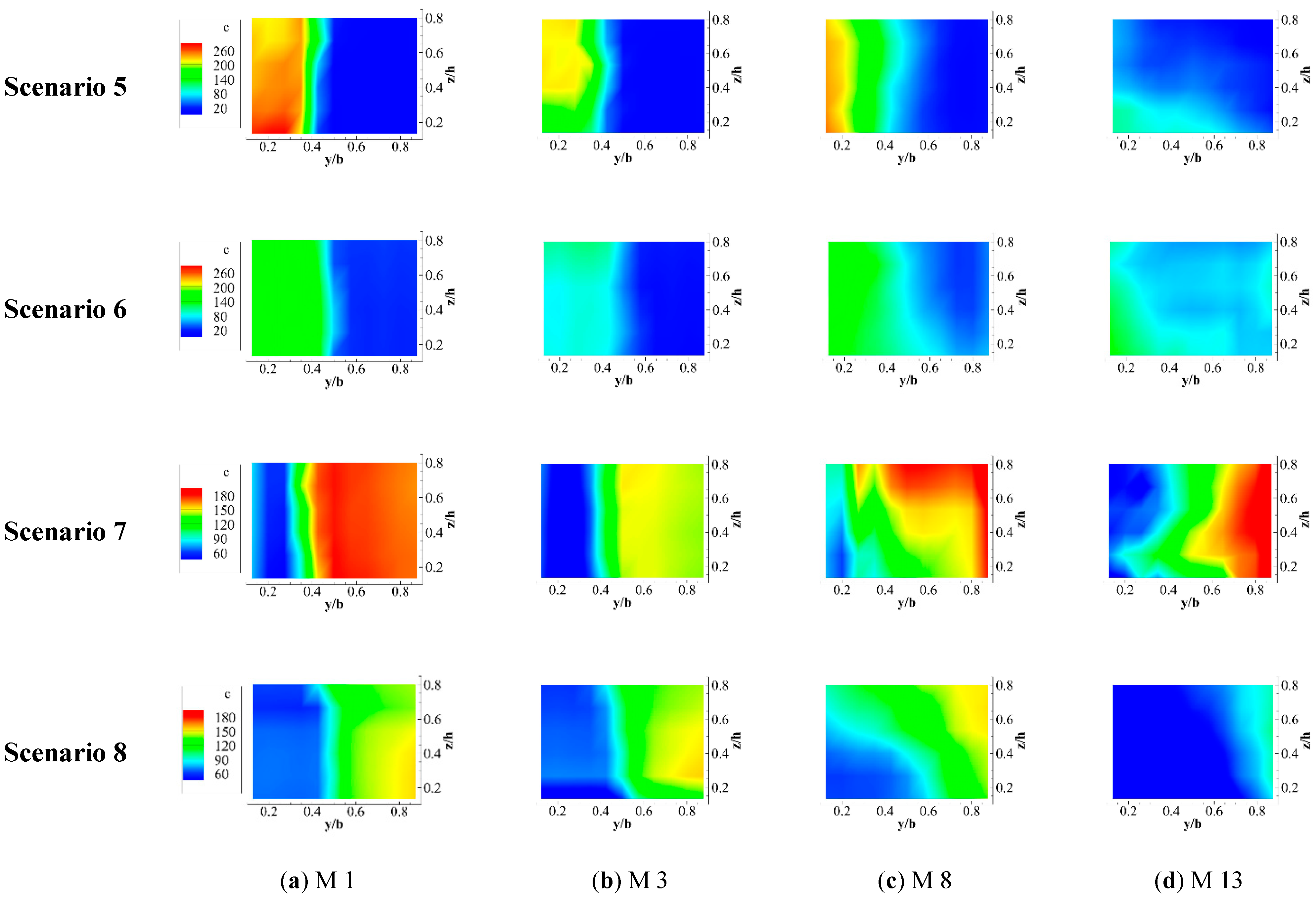
3.2. Transport of Contaminants at Channel Confluences
3.2.1. Different Discharge Manners and Locations
3.2.2. Different Discharge Ratios
4. Conclusions
5. Patents
Author Contributions
Funding
Acknowledgments
Conflicts of Interest
References
- Ghostine, R.; Vazquez, J.; Terfous, A.; Rivière, N.; Ghenaim, A.; Mosé, R. A comparative study of 1D and 2D approaches for simulating flows at right angled dividing junctions. Appl. Math. Comput. 2013, 219, 5070–5082. [Google Scholar] [CrossRef]
- Yuan, S.; Tang, H.; Xiao, Y.; Chen, X.; Xia, Y.; Jiang, Z. Spatial variability of phosphorus adsorption in surface sediment at channel confluences: Field and laboratory experimental evidence. J. Hydro-Environ. Res. 2018, 18, 25–36. [Google Scholar] [CrossRef]
- Konsoer, K.M.; Rhoads, B.L. Spatial–temporal structure of mixing interface turbulence at two large river confluences. Environ. Fluid Mech. 2014, 14, 1043–1070. [Google Scholar] [CrossRef]
- Best, J.L. Flow Dynamics at River Channel Confluences: Implications for Sediment Transport and Bed Morphology; SEPM: Tulsa, OK, USA, 1987. [Google Scholar]
- Best, J.L.; Reid, I. Separation Zone at Open-Channel Junctions. J. Hydraul. Eng. 1984, 110, 1588–1594. [Google Scholar] [CrossRef]
- Qing-Yuan, Y.; Xian-Ye, W.; Wei-Zhen, L.; Xie-Kang, W. Experimental Study on Characteristics of Separation Zone in Confluence Zones in Rivers. J. Hydrol. Eng. 2009, 14, 166–171. [Google Scholar] [CrossRef]
- Best, J.L. Sediment transport and bed morphology at river channel confluences. Sedimentology 1988, 35, 481–498. [Google Scholar] [CrossRef]
- Best, J.L.; Roy, A.G. Mixing-Layer Distortion at the Confluence of Channels of Different Depth. Nature 1991, 350, 411. [Google Scholar] [CrossRef]
- Biron, P.; Best, J.L.; Ror, A.G. Effects of Bed Discordance on Flow Dynamics at Open Channel Confluences. J. Hydraul. Eng. 1996, 122, 676–682. [Google Scholar] [CrossRef]
- Biron, P.; Boy, A.G.; Best, J.L. Turbulent flow structure at concordant and discordant open-channel confluences. Exp. Fluids 1996, 21, 437–446. [Google Scholar] [CrossRef]
- Wu, F.-S.; Hsu, C.-C.; Lee, W.-J. Flow at 90° Equal-Width Open-Channel Junction. J. Hydraul. Eng. 1998, 124, 186–191. [Google Scholar]
- Hsu, C.-C.; Chang, C.-H.; Lee, W.-J. Subcritical Open-Channel Junction Flow. J. Hydraulic Eng. 1998, 124, 847–855. [Google Scholar] [CrossRef]
- Weber, L.J.; Schumate, E.D.; Mawer, N. Experiments on flow at a 90 degrees open-channel junction. J. Hydraul. Eng.-ASCE 2001, 127, 340–350. [Google Scholar] [CrossRef]
- Tong-huan, L.; Wei, G.; Lei, Z. Experimental study of the vdocity profile at 90° open channel confluence. Adv. Water Sci. 2009, 20, 485–489. [Google Scholar]
- Biswal, S.K.; Mohapatra, P.; Muralidhar, K. Hydraulics of combining flow in a right-angled compound open channel junction. Sadhana-Acad. Proc. Eng. Sci. 2016, 41, 97–110. [Google Scholar] [CrossRef]
- Yuan, S.; Tang, H.; Xiao, Y.; Qiu, X.; Zhang, H.; Yu, D. Turbulent flow structure at a 90-degree open channel confluence: Accounting for the distortion of the shear layer. J. Hydro-Environ. Res. 2016, 12, 130–147. [Google Scholar] [CrossRef]
- Song, C.G.; Seo, I.W.; Kim, Y.D. Analysis of secondary current effect in the modeling of shallow flow in open channels. Adv. Water Resour. 2012, 41, 29–48. [Google Scholar] [CrossRef]
- Schindfessel, L.; Creelle, S.; De Mulder, T. Flow Patterns in an Open Channel Confluence with Increasingly Dominant Tributary Inflow. Water 2015, 7, 4724–4751. [Google Scholar] [CrossRef] [Green Version]
- Biron, P.M.; Ramamurthy, A.S.; Han, S. Three-dimensional numerical modeling of mixing at river confluences. J. Hydraulic Eng.-ASCE 2004, 130, 243–253. [Google Scholar] [CrossRef]
- Azevedo, I.C.; Bordalo, A.A.; Duarte, P.M. Influence of river discharge patterns on the hydrodynamics and potential contaminant dispersion in the Douro estuary (Portugal). Water Res. 2010, 44, 3133–3146. [Google Scholar] [CrossRef]
- Liu, M.; Chen, X.; Dong, Z. Effect of Lateral Inflow of Branch on the Characteristics of Flow and Pollutant of the Mainstream in Tidal River. In Proceedings of the 4th International Yellow River Forum on Ecological Civilization and River Ethics; Huanghe Water Conservancy Press: Zhengzhou, China, 2010; pp. 134–141. [Google Scholar]
- Tang, H.; Zhang, H.; Yuan, S. Hydrodynamics and contaminant transport on a degraded bed at a 90-degree channel confluence. Environ. Fluid Mech. 2017, 18, 443–463. [Google Scholar] [CrossRef]
- Weidong, G.; Xiaogang, W.; Jiwen, Y.; Tianen, Y.; Yue, L. Research of Hydraulic Characteristics of “Y”shaped Junction. Water Resour. Power 2005, 23, 53–56. [Google Scholar]
- Rhoads, B.L.; Sukhodolov, A.N. Field investigation of three-dimensional flow structure at stream confluences: 1. Thermal mixing and time-averaged velocities. Water Resour. Res. 2001, 37, 2393–2410. [Google Scholar] [CrossRef] [Green Version]
- Geberemariam, T.K. Numerical Analysis of Stormwater Flow Conditions and Separation Zone at Open-Channel Junctions. J. Irrig. Drain. Eng. 2017, 143, 5016009. [Google Scholar] [CrossRef]
- Rhoads, B.L.; Sukhodolov, A.N. Spatial and temporal structure of shear layer turbulence at a stream confluence. Water Resour. Res. 2004, 40. [Google Scholar] [CrossRef] [Green Version]
- Sanjou, M.; Nezu, I. Hydrodynamic characteristics and related mass-transfer properties in open-channel flows with rectangular embayment zone. Environ. Fluid Mech. 2013, 13, 527–555. [Google Scholar] [CrossRef] [Green Version]
- Coelho, M. Experimental determination of free surface levels at open-channel junctions. J. Hydraul. Res. 2015, 53, 394–399. [Google Scholar] [CrossRef]
- Nanía, L.S.; Gómez, M.; Gonzalo, R. Influence of Channel Width on Flow Distribution in Four-Branch Junctions with Supercritical Flow: Experimental Approach. J. Hydraul. Eng. 2014, 140, 77–88. [Google Scholar] [CrossRef]
- Yang, Q.Y.; Liu, T.H.; Lu, W.Z.; Wang, X.K. Numerical Simulation of Confluence Flow in Open Channel with Dynamic Meshes Techniques. Adv. Mech. Eng. 2013, 5, 860431. [Google Scholar] [CrossRef]
- Sharifipour, M.; Bonakdari, H.; Zaji, A.H.; Shamshirband, S. Numerical investigation of flow field and flowmeter accuracy in open-channel junctions. Eng. Appl. Comput. Fluid Mech. 2015, 9, 280–290. [Google Scholar] [CrossRef]
- Ferguson, R.; Hoey, T. Effects of Tributaries on Main-ChannelGeomorphology. In River Confluences, Tributaries and the Fluvial Network; John Wiley & Sons: Hoboken, NJ, USA, 2008; pp. 193–208. [Google Scholar]


| Y-shaped Confluence | Left Branch Mean Width (m) | Right Branch Mean Width (m) | Mainstream Mean Width (m) | Confluence Angle (°) |
|---|---|---|---|---|
| 1 | 100.21 | 107.81 | 198.81 | 58.59 |
| 2 | 69.06 | 80.15 | 106.15 | 48.35 |
| 3 | 27.81 | 30.83 | 54.65 | 30.81 |
| 4 | 98.23 | 100.88 | 163.15 | 60.98 |
| 5 | 54.14 | 73.18 | 100.88 | 69.27 |
| 6 | 33.31 | 48.02 | 54.15 | 75.03 |
| 7 | 32.61 | 38.17 | 44.63 | 92.73 |
| 8 | 29.56 | 40.30 | 74.14 | 45.57 |
| Average value | 55.62 | 64.92 | 99.57 | 60.17 |
| Scenario | Discharge (m³/h) | Contaminant Discharge Methods | Contaminant Discharge Position | |
|---|---|---|---|---|
| Left branch | Right branch | |||
| 1 | 10 | 20 | point source | The outer bank of the left branch |
| 2 | 10 | 20 | point source | The inner bank of the left branch |
| 3 | 10 | 20 | point source | The outer bank of the left branch |
| 4 | 10 | 20 | point source | The inner bank of the left branch |
| 5 | 10 | 20 | line source | The full section of left branch |
| 6 | 10 | 20 | line source | The full section of right branch |
| 7 | 20 | 20 | line source | The full section of left branch |
| 8 | 20 | 20 | line source | The full section of right branch |
© 2019 by the authors. Licensee MDPI, Basel, Switzerland. This article is an open access article distributed under the terms and conditions of the Creative Commons Attribution (CC BY) license (http://creativecommons.org/licenses/by/4.0/).
Share and Cite
Liu, X.; Li, L.; Hua, Z.; Tu, Q.; Yang, T.; Zhang, Y. Flow Dynamics and Contaminant Transport in Y-Shaped River Channel Confluences. Int. J. Environ. Res. Public Health 2019, 16, 572. https://0-doi-org.brum.beds.ac.uk/10.3390/ijerph16040572
Liu X, Li L, Hua Z, Tu Q, Yang T, Zhang Y. Flow Dynamics and Contaminant Transport in Y-Shaped River Channel Confluences. International Journal of Environmental Research and Public Health. 2019; 16(4):572. https://0-doi-org.brum.beds.ac.uk/10.3390/ijerph16040572
Chicago/Turabian StyleLiu, Xiaodong, Lingqi Li, Zulin Hua, Qile Tu, Ting Yang, and Yuan Zhang. 2019. "Flow Dynamics and Contaminant Transport in Y-Shaped River Channel Confluences" International Journal of Environmental Research and Public Health 16, no. 4: 572. https://0-doi-org.brum.beds.ac.uk/10.3390/ijerph16040572