
Long-Term Assessment of Surface Water Quality in a Highly Managed Estuary Basin


Abstract
:1. Introduction
2. Materials and Methods
2.1. Study Setting
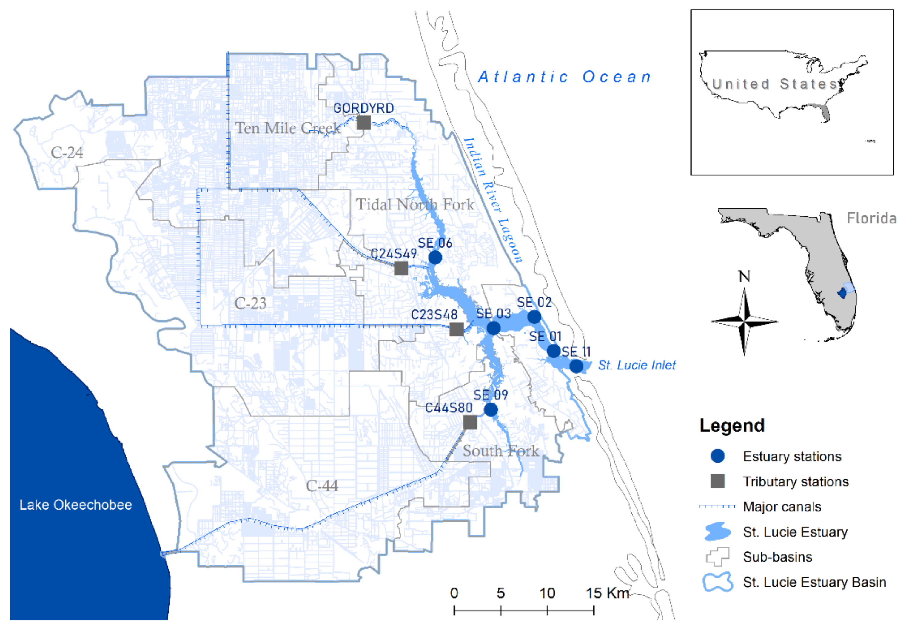
2.1.1. Estuary
2.1.2. Land Cover
2.2. Data
2.2.1. Rainfall and Flow
2.2.2. Water Quality Data
2.3. Statistical Methods
2.3.1. Assessment of Rainfall and Flow Data
2.3.2. Assessment of Physicochemical Variables
2.3.3. Principal Component Analysis (PCA)
2.3.4. Correlation and Trend Analyses
3. Results
3.1. Assessment of Rainfall and Flow Data
3.2. Assessment of Physicochemical Variables
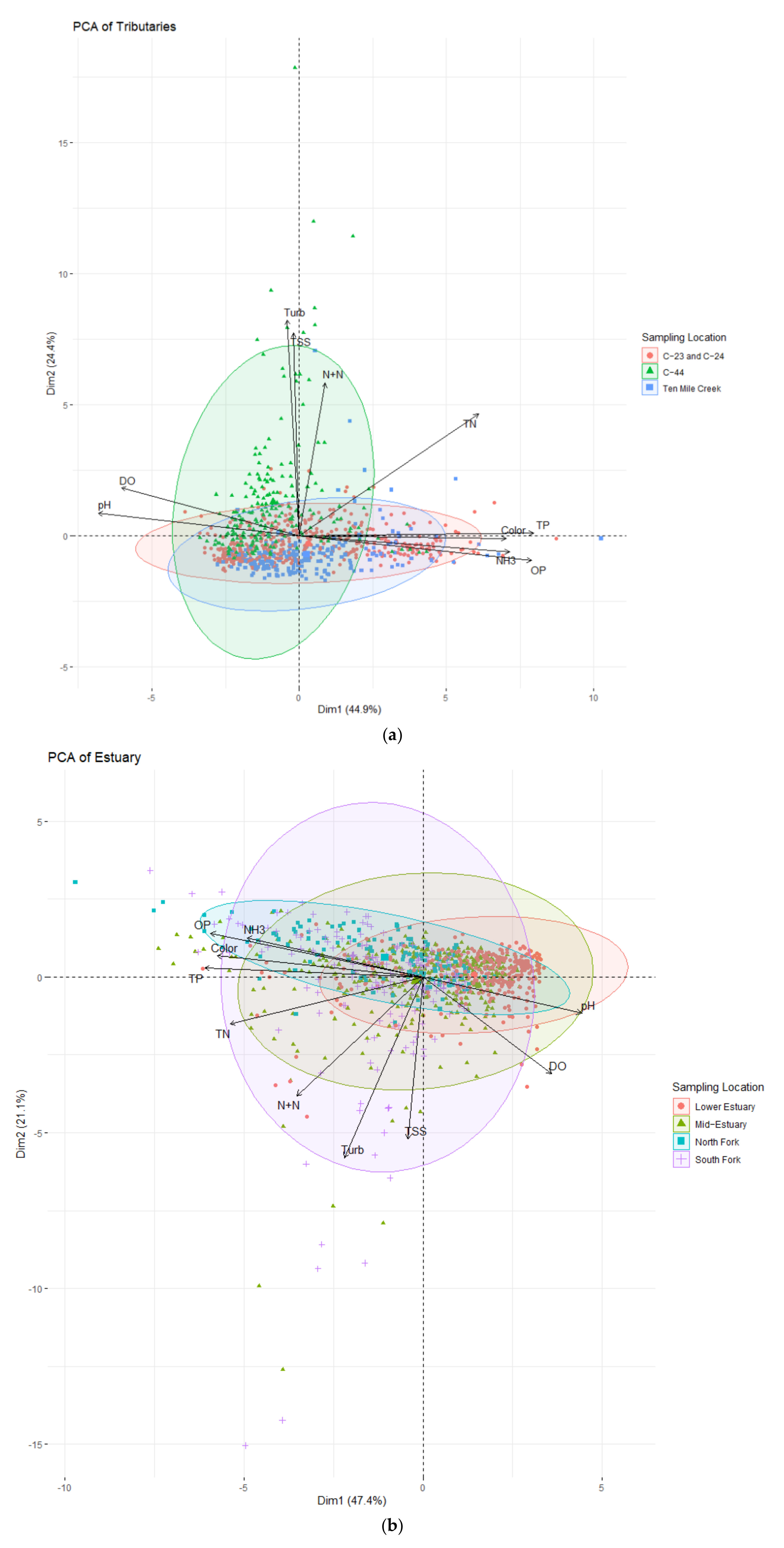
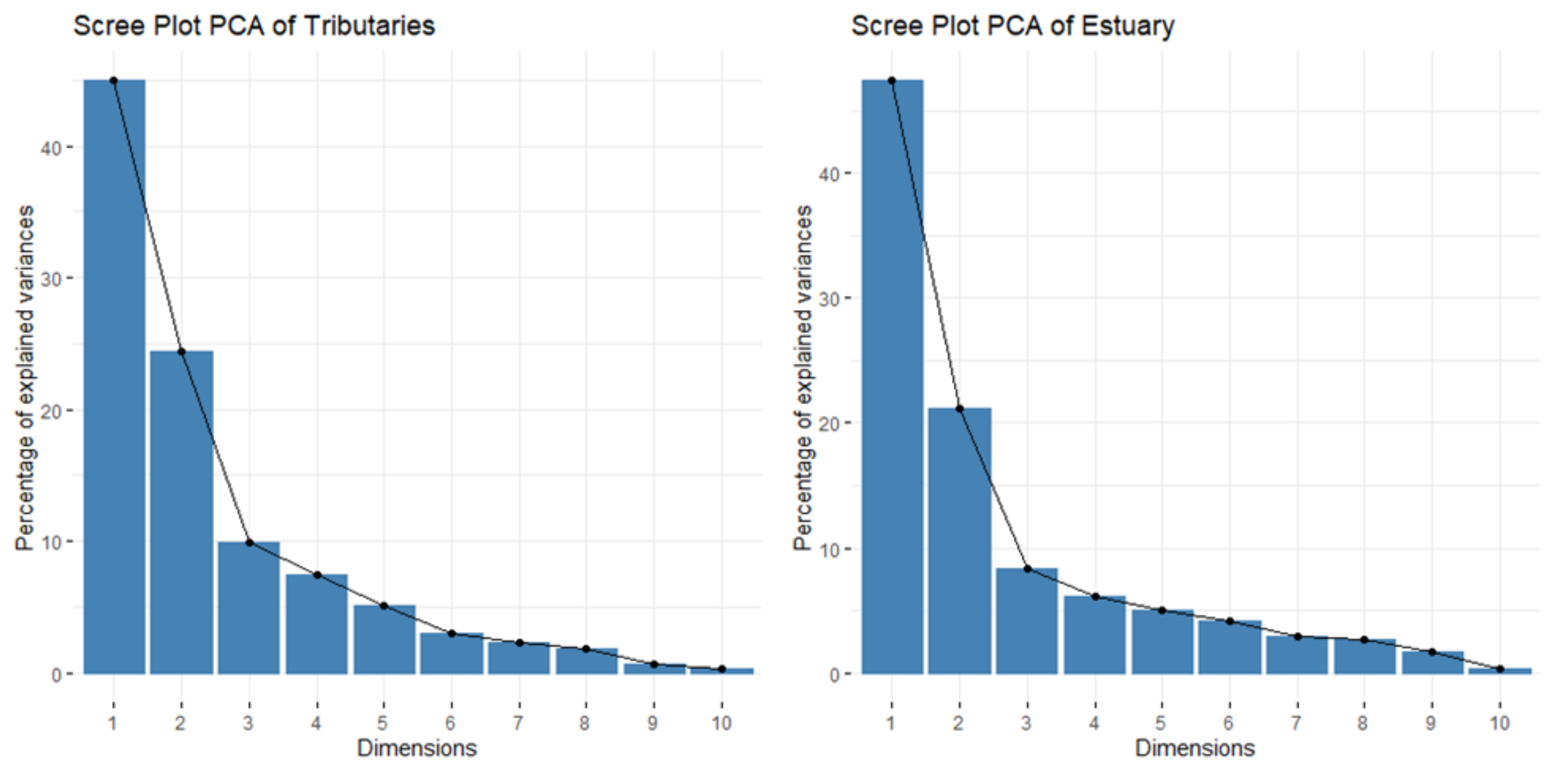
3.3. Principal Component Analysis (PCA)
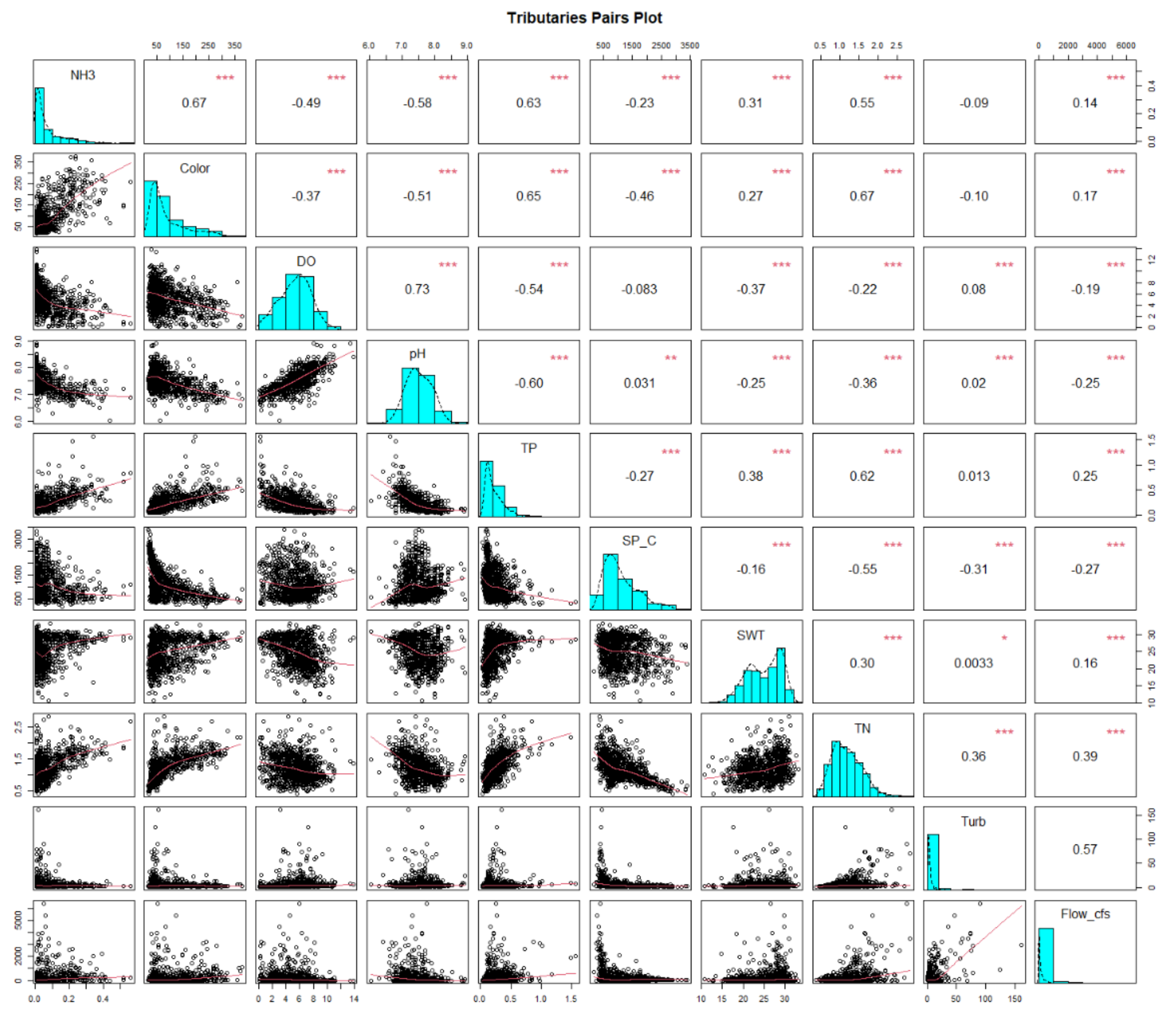
3.4. Correlation of Physicochemical Variables
3.5. Trend Analysis
4. Discussion
4.1. Seasonality of Freshwater Inputs
4.2. Seasonality of Water Quality
4.3. Spatial Variability of Physicochemical Variables
4.4. Monotonic Trends
5. Conclusions
Supplementary Materials
Author Contributions
Funding
Institutional Review Board Statement
Informed Consent Statement
Data Availability Statement
Acknowledgments
Conflicts of Interest
References
- Dodds, W.K.; Bouska, W.W.; Eitzmann, J.L.; Pilger, T.J.; Pitts, K.L.; Riley, A.J.; Schloesser, J.T.; Thornbrugh, D.J. Eutrophication of U. S. Freshwaters: Analysis of Potential Economic Damages. Environ. Sci. Technol. 2009, 43, 12–19. [Google Scholar] [CrossRef] [PubMed] [Green Version]
- Costanza, R.; de Groot, R.; Sutton, P.; van der Ploeg, S.; Anderson, S.J.; Kubiszewski, I.; Farber, S.; Turner, R.K. Changes in the Global Value of Ecosystem Services. Glob. Environ. Chang. 2014, 26, 152–158. [Google Scholar] [CrossRef]
- Bricker, S.B.; Longstaff, B.; Dennison, W.; Jones, A.; Boicourt, K.; Wicks, C.; Woerner, J. Effects of Nutrient Enrichment in the Nation’s Estuaries: A Decade of Change. Harmful Algae 2008, 8, 21–32. [Google Scholar] [CrossRef]
- Hopkinson, C.S.; Vallino, J.J. The Relationships among Man’s Activities in Watersheds and Estuaries: A Model of Runoff Effects on Patterns of Estuarine Community Metabolism. Estuaries 1995, 18, 598–621. [Google Scholar] [CrossRef]
- Le Moal, M.; Gascuel-Odoux, C.; Ménesguen, A.; Souchon, Y.; Étrillard, C.; Levain, A.; Moatar, F.; Pannard, A.; Souchu, P.; Lefebvre, A.; et al. Eutrophication: A New Wine in an Old Bottle? Sci. Total Environ. 2019, 651, 1–11. [Google Scholar] [CrossRef] [PubMed] [Green Version]
- Benson, N.G. The Freshwater-Inflow-To-Estuaries Issue. Fisheries 1981, 6, 1971–1973. [Google Scholar] [CrossRef]
- Kemp, W.M.; Boynton, W.R.; Adolf, J.E.; Boesch, D.F.; Boicourt, W.C.; Brush, G.; Cornwell, J.C.; Fisher, T.R.; Glibert, P.M.; Hagy, J.D.; et al. Eutrophication of Chesapeake Bay: Historical Trends and Ecological Interactions. Mar. Ecol. Prog. Ser. 2005, 303, 1–29. [Google Scholar] [CrossRef]
- Poff, N.L.R.; Bledsoe, B.P.; Cuhaciyan, C.O. Hydrologic Variation with Land Use across the Contiguous United States: Geomorphic and Ecological Consequences for Stream Ecosystems. Geomorphology 2006, 79, 264–285. [Google Scholar] [CrossRef]
- Lee, S.Y.; Dunn, R.J.K.; Young, R.A.; Connolly, R.M.; Dale, P.E.R.; Dehayr, R.; Lemckert, C.J.; McKinnon, S.; Powell, B.; Teasdale, P.R.; et al. Impact of Urbanization on Coastal Wetland Structure and Function. Austral Ecol. 2006, 31, 149–163. [Google Scholar] [CrossRef]
- Glibert, P.M. Eutrophication, Harmful Algae and Biodiversity—Challenging Paradigms in a World of Complex Nutrient Changes. Mar. Pollut. Bull. 2017, 124, 591–606. [Google Scholar] [CrossRef]
- Briciu-Burghina, C.; Sullivan, T.; Chapman, J.; Regan, F. Continuous High-Frequency Monitoring of Estuarine Water Quality as a Decision Support Tool: A Dublin Port Case Study. Environ. Monit. Assess. 2014, 186, 5561–5580. [Google Scholar] [CrossRef] [PubMed]
- Arabi, B.; Salama, M.S.; Pitarch, J.; Verhoef, W. Integration of In-Situ and Multi-Sensor Satellite Observations for Long-Term Water Quality Monitoring in Coastal Areas. Remote Sens. Environ. 2020, 239, 111632. [Google Scholar] [CrossRef]
- Dodds, W.K.; Smith, V.H. Nitrogen, Phosphorus, and Eutrophication in Streams. Inland Waters 2016, 6, 155–164. [Google Scholar] [CrossRef]
- Grizzetti, B.; Bouraoui, F.; de Marsily, G.; Bidoglio, G. A Statistical Method for Source Apportionment of Riverine Nitrogen Loads. J. Hydrol. 2005, 304, 302–315. [Google Scholar] [CrossRef]
- Bachmann, R.W.; Bigham, D.L.; Hoyer, M.V.; Canfield, D.E. Factors Determining the Distributions of Total Phosphorus, Total Nitrogen, and Chlorophyll a in Florida Lakes. Lake Reserv. Manag. 2012, 28, 10–26. [Google Scholar] [CrossRef]
- Hajigholizadeh, M.; Melesse, A.M. Assortment and Spatiotemporal Analysis of Surface Water Quality Using Cluster and Discriminant Analyses. Catena 2017, 151, 247–258. [Google Scholar] [CrossRef]
- Basnyat, P.; Teeter, L.D.; Flynn, K.; Lockaby, B.G. Relationships Between Landscape Characteristics and Nonpoint Source Pollution Inputs to Coastal Estuaries. Environ. Manag. 1999, 23, 539–549. [Google Scholar] [CrossRef]
- Shrestha, S.; Kazama, F.; Newham, L.T.H. A Framework for Estimating Pollutant Export Coefficients from Long-Term in-Stream Water Quality Monitoring Data. Environ. Model. Softw. 2008, 23, 182–194. [Google Scholar] [CrossRef]
- Trim, A.H.; Marcus, J.M. Integration of Long-Term Fish Kill Data with Ambient Water Quality Monitoring Data and Application to Water Quality Management. Environ. Manag. 1990, 14, 389–396. [Google Scholar] [CrossRef]
- Stets, E.G.; Kelly, V.J.; Crawford, C.G. Regional and Temporal Differences in Nitrate Trends Discerned from Long-Term Water Quality Monitoring Data. JAWRA J. Am. Water Resour. Assoc. 2015, 51, 1394–1407. [Google Scholar] [CrossRef]
- Boyer, J.N.; Fourqurean, J.W.; Jones, R.D. Seasonal and Long-Term Trends in the Water Quality of Florida Bay (1989–1997). Estuaries 1999, 22, 417–430. [Google Scholar] [CrossRef]
- Bugica, K.; Sterba-Boatwright, B.; Wetz, M.S. Water Quality Trends in Texas Estuaries. Mar. Pollut. Bull. 2020, 152, 110903. [Google Scholar] [CrossRef] [PubMed]
- Romero, E.; Le Gendre, R.; Garnier, J.; Billen, G.; Fisson, C.; Silvestre, M.; Riou, P. Long-Term Water Quality in the Lower Seine: Lessons Learned over 4 Decades of Monitoring. Environ. Sci. Policy 2016, 58, 141–154. [Google Scholar] [CrossRef] [Green Version]
- South Florida Water Management District. Technical Documentation to Support Development of Minimum Flows for the St. Lucie River and Estuary; South Florida Water Management District: West Palm Beach, FL, USA, 2002; p. 136.
- Florida Department of Environmental Protection. St. Lucie River and Estuary Basin Management Action Plan; Florida Department of Environmental Protection: Tallahassee, FL, USA, 2020; p. 216.
- Chamberlain, R.; Hayward, D. Evaluation of Water Quality and Monitoring in the St. Lucie Estuary, Florida. J. Am. Water Resour. Assoc. 1996, 32, 681–696. [Google Scholar] [CrossRef]
- Wilson, C.; Scotto, L.; Scarpa, J.; Volety, A.; Laramore, S.; Haunert, D. Survey of Water Quality, Oyster Reproduction and Oyster Health Status in the St. Lucie Estuary. J. Shellfish Res. 2005, 24, 157–165. [Google Scholar] [CrossRef]
- Morris, F.W. Bathymetry of the St. Lucie Estuary; South Florida Water Management District: West Palm Beach, FL, USA, 1986; p. 140.
- Doering, P.H. Temporal Variability of Water Quality in the St. Lucie Estuary, South Florida. J. Am. Water Resour. Assoc. 1996, 32, 1293–1306. [Google Scholar] [CrossRef]
- Qian, Y.; Migliaccio, K.W.; Wan, Y.; Li, Y.C.; Chin, D. Seasonality of Selected Surface Water Constituents in the Indian River Lagoon, Florida. J. Environ. Qual. 2007, 36, 416–425. [Google Scholar] [CrossRef]
- Sepulveda, N.; Tiedeman, C.; O’Reilly, A.M.; Davis, J.B.; Burger, P. Groundwater Flow and Water Budget in the Surficial and Floridan Aquifer Systems in East-Central Florida; United States Department of the Interior: Reston, VA, USA, 2012; p. 232.
- Hampel, J.J.; McCarthy, M.J.; Aalto, S.L.; Newell, S.E. Hurricane Disturbance Stimulated Nitrification and Altered Ammonia Oxidizer Community Structure in Lake Okeechobee and St. Lucie Estuary (Florida). Front. Microbiol. 2020, 11, 1541. [Google Scholar] [CrossRef]
- Kramer, B.J.; Davis, T.W.; Meyer, K.A.; Rosen, B.H.; Goleski, J.A.; Dick, G.J.; Oh, G.; Gobler, C.J. Nitrogen Limitation, Toxin Synthesis Potential, and Toxicity of Cyanobacterial Populations in Lake Okeechobee and the St. Lucie River Estuary, Florida, during the 2016 State of Emergency Event. PLoS ONE 2018, 13, e0196278. [Google Scholar] [CrossRef] [Green Version]
- Lapointe, B.E.; Herren, L.W.; Paule, A.L. Septic Systems Contribute to Nutrient Pollution and Harmful Algal Blooms in the St. Lucie Estuary, Southeast Florida, USA. Harmful Algae 2017, 70, 1–22. [Google Scholar] [CrossRef]
- Oehrle, S.; Rodriguez-Matos, M.; Cartamil, M.; Zavala, C.; Rein, K.S. Toxin Composition of the 2016 Microcystis Aeruginosa Bloom in the St. Lucie Estuary, Florida. Toxicon 2017, 138, 169–172. [Google Scholar] [CrossRef]
- Florida Department of Environmental Protection. St. Lucie River and Estuary Basin Management Action for the Implementation of Total Maximum Daily Loads for Nutrients and Dissolved Oxygen; Florida Department of Environmental Protection: Tallahassee, FL, USA, 2013; p. 114.
- Armstrong, C.; Zheng, F.; Wachnicka, A.; Khan, A.; Chen, Z.; Baldwin, L. C: St. Lucie and Caloosahatchee River Watersheds Annual Report. In South Florida Environmental Report; Chapter 8; South Florida Water Management District: West Palm Beach, FL, USA, 2019; pp. 1–44. [Google Scholar]
- Byrne, B.M.J.; Patino, E.; Norton, G.A. Hydrologic Data Summary for the St. Lucie River Estuary, Martin and St. Lucie Counties, Florida, 1998–2001; USGS: Reston, VA, USA, 2004; p. 19.
- Duan, W.; He, B.; Nover, D.; Yang, G.; Chen, W.; Meng, H.; Zou, S.; Liu, C. Water Quality Assessment and Pollution Source Identification of the Eastern Poyang Lake Basin Using Multivariate Statistical Methods. Sustainability 2016, 8, 133. [Google Scholar] [CrossRef] [Green Version]
- Phlips, E.J.; Badylak, S.; Grosskopf, T. Factors Affecting the Abundance of Phytoplankton in a Restricted Subtropical Lagoon, the Indian River Lagoon, Florida, USA. Estuar. Coast. Shelf Sci. 2002, 55, 385–402. [Google Scholar] [CrossRef]
- Ji, Z.G.; Hu, G.; Shen, J.; Wan, Y. Three-Dimensional Modeling of Hydrodynamic Processes in the St. Lucie Estuary. Estuar. Coast. Shelf Sci. 2007, 73, 188–200. [Google Scholar] [CrossRef]
- Steward, J.; Higman, J.; Morris, F.; Sargent, W.; Virnstein, R.; Lund, F.; VanArman, J. Surface Water Improvement and Management (SWIM) Plan for the Indian River Lagoon; South Florida Water Management District: West Palm Beach, FL, USA, 1989; p. 109.
- United States Geological Survey. [Dataset] The National Land Cover Database. Available online: https://www.mrlc.gov/data?f%5B0%5D=category%3Aland%20cover&f%5B1%5D=year%3A2016 (accessed on 15 May 2020).
- South Florida Water Management District. [Dataset] Radar Rainfall. Available online: https://apps.sfwmd.gov/nexrad2/nrdmain.action (accessed on 15 May 2020).
- South Florida Water Management District. [Dataset] DBHYDRO Surface Water Hydrological & Physical Data-Surface Water Data. Available online: https://my.sfwmd.gov/dbhydroplsql/show_dbkey_info.web_qry_form?v_category=SW&v_js_flag=Y&v_paramStr=station&v_param_value= (accessed on 15 May 2020).
- South Florida Water Management District. [Dataset] DBHYDRO Water Quality Data-Grab Samples. Available online: https://my.sfwmd.gov/dbhydroplsql/water_quality_interface.main_page (accessed on 15 January 2020).
- Rice, E.W.; Baird, R.B.; Eaton, A.D. Standard Methods for the Examination of Water and Wastewater, 23rd ed.; Water Environment Federation: Alexandria, VA, USA; American Public Health Association: Washington, DC, USA; American Water Works Association: Denver, CO, USA, 2017; p. 1624. ISBN 978-0-87553-287-5. [Google Scholar]
- Walker, R. Total Nitrogen Methods Fact Sheet. In Proceedings of the Technical Oversight Committee; South Florida Water Management District: West Palm Beach, FL, USA, 2014; p. 5. [Google Scholar]
- South Florida Water Management District. DBHYDRO Browser User’s Guide; South Florida Water Management District: West Palm Beach, FL, USA, 2020; p. 106.
- Helsel, D.R.; Cohn, T.A. Estimation of Descriptive Statistics for Multiply Censored Water Quality Data. Water Resour. Res. 1988, 24, 1997–2004. [Google Scholar] [CrossRef]
- Helsel, D.R. Statistics for Censored Environmental Data Using Minitab and R, 2nd ed.; John Wiley & Sons, Inc.: New York, NY, USA, 2012; pp. 62–69. ISBN 9781118162781. [Google Scholar]
- Kendall, M.G. A New Measure of Rank Correlation. Biometrika 1938, 30, 81–93. [Google Scholar] [CrossRef]
- Bartholomay, R.C.; Davis, L.C.; Fisher, J.C.; Tucker, B.J.; Raben, F.A. Water-Quality Characteristics and Trends for Selected Sites At and Near the Idaho National Laboratory, Idaho, 1949–2009; United States Geological Survey: Reston, VA, USA, 2012; p. 78.
- Russell, I.A. Spatio-Temporal Variability of Surface Water Quality Parameters in a South African Estuarine Lake System. Afr. J. Aquat. Sci. 2013, 38, 53–66. [Google Scholar] [CrossRef]
- Meals, D.W.; Spooner, J.; Dressing, S.A.; Harcum, J. Statistical Analysis for Monotonic Trends; United States Environmental Protection Agency: Fairfax, VA, USA, 2011; p. 23.
- Helsel, D.R.; Hirsch, R.M.; Ryberg, K.R.; Archfield, S.A.; Gilroy, E.J. Statistical Methods in Water Resources: U.S. Geological Survey Techniques and Methods; Book 4, Chapter A3; United States Geological Survey: Reston, VA, USA, 2020; p. 458. ISSN 2328-7055.
- De Souza Pereira, M.A.; Cavalheri, P.S.; de Oliveira, M.Â.C.; Magalhães Filho, F.J.C. A Multivariate Statistical Approach to the Integration of Different Land-Uses, Seasons, and Water Quality as Water Resources Management Tool. Environ. Monit. Assess. 2019, 191, 539. [Google Scholar] [CrossRef]
- Vega, M.; Pardo, R.; Barrado, E.; Debán, L. Assessment of Seasonal and Polluting Effects on the Quality of River Water by Exploratory Data Analysis. Water Res. 1998, 32, 3581–3592. [Google Scholar] [CrossRef]
- Ryberg, K.R. Multivariate Statistical Analysis in Water Quality. In Proceedings of the National Water Quality Monitoring Council Webinar Series; Fully-online; United States Geological Survey: Reston, VA, USA, 2017; p. 35. [Google Scholar]
- Hirsch, R.M.; Slack, J.R.; Smith, R.A. Techniques of Trend Analysis for Monthly Water Quality Data. Water Resour. Res. 1982, 18, 107–121. [Google Scholar] [CrossRef] [Green Version]
- Mann, H.B. Nonparametric Tests Against Trend. Econometrica 1945, 13, 245–259. [Google Scholar] [CrossRef]
- Campion, W.M.; Rubin, D.B. Multiple Imputation for Nonresponse in Surveys. J. Mark. Res. 1989, 26, 485. [Google Scholar] [CrossRef]
- Sen, P.K. Estimates of the Regression Coefficient Based on Kendall’s Tau. Source J. Am. Stat. Assoc. 1968, 63, 1379–1389. [Google Scholar] [CrossRef]
- Buzzelli, C.; Wan, Y.; Doering, P.H.; Boyer, J.N. Seasonal Dissolved Inorganic Nitrogen and Phosphorus Budgets for Two Sub-Tropical Estuaries in South Florida, USA. Biogeosciences 2013, 10, 6721–6736. [Google Scholar] [CrossRef] [Green Version]
- Abiy, A.Z.; Melesse, A.M.; Abtew, W. Teleconnection of Regional Drought to ENSO, PDO, and AMO: Southern Florida and the Everglades. Atmosphere 2019, 10, 295. [Google Scholar] [CrossRef] [Green Version]
- Alexander, M.A.; Halimeda Kilbourne, K.; Nye, J.A. Climate Variability during Warm and Cold Phases of the Atlantic Multidecadal Oscillation (AMO) 1871-2008. J. Mar. Syst. 2014, 133, 14–26. [Google Scholar] [CrossRef]
- Irizarry-Ortiz, M.M.; Obeysekera, J.; Park, J.; Trimble, P.; Barnes, J.; Park-Said, W.; Gadzinski, E. Historical Trends in Florida Temperature and Precipitation. Hydrol. Process. 2013, 27, 2225–2246. [Google Scholar] [CrossRef]
- Martinez, C.J.; Maleski, J.J.; Miller, M.F. Trends in Precipitation and Temperature in Florida, USA. J. Hydrol. 2012, 452–453, 259–281. [Google Scholar] [CrossRef]
- Abiy, A.Z.; Melesse, A.M.; Abtew, W.; Whitman, D. Rainfall Trend and Variability in Southeast Florida: Implications for Freshwater Availability in the Everglades. PLoS ONE 2019, 14, e0212008. [Google Scholar] [CrossRef] [Green Version]
- Cooper, R.M.; Ortel, T.W. An Atlas of St. Lucie County Surface Water Management Basins: Technical Memorandum; South Florida Water Management District: West Palm Beach, FL, USA, 1988; p. 40.
- Wilcock, D.; Wilcock, F. Modelling the Hydrological Impacts of Channelization on Streamflow Characteristics in a Northern Ireland Catchment. In Proceedings of the Modelling and Management of Sustainable Basin-scale Water Resource Systems, Boulder, CO, USA, 1–14 July 1995; IAHS: Wallingford, CT, USA, 1995; pp. 41–48. [Google Scholar]
- Li, L.; He, Z.; Li, Z.; Zhang, S.; Li, S.; Wan, Y.; Stoffella, P.J. Spatial and Temporal Variation of Nitrogen Concentration and Speciation in Runoff and Storm Water in the Indian River Watershed, South Florida. Environ. Sci. Pollut. Res. 2016, 23, 19561–19569. [Google Scholar] [CrossRef]
- Li, L.; He, Z.; Li, Z.; Li, S.; Wan, Y.; Stoffella, P.J. Spatiotemporal Change of Phosphorous Speciation and Concentration in Stormwater in the St. Lucie Estuary Watershed, South Florida. Chemosphere 2017, 172, 488–495. [Google Scholar] [CrossRef]
- Millie, D.F.; Carrick, H.J.; Doering, P.H.; Steidinger, K.A. Intra-Annual Variability of Water Quality and Phytoplankton in the North Fork of the St. Lucie River Estuary, Florida (USA): A Quantitative Assessment. Estuar. Coast. Shelf Sci. 2004, 61, 137–149. [Google Scholar] [CrossRef]
- Barile, P.J. Widespread Sewage Pollution of the Indian River Lagoon System, Florida (USA) Resolved by Spatial Analyses of Macroalgal Biogeochemistry. Mar. Pollut. Bull. 2018, 128, 557–574. [Google Scholar] [CrossRef] [PubMed]
- Lapointe, B.E.; Herren, L.W.; Bedford, B.J. Effects of Hurricanes, Land Use, and Water Management on Nutrient and Microbial Pollution: St. Lucie Estuary, Southeast Florida. J. Coast. Res. 2012, 285, 1345–1361. [Google Scholar] [CrossRef]
- Badruzzaman, M.; Pinzon, J.; Oppenheimer, J.; Jacangelo, J.G. Sources of Nutrients Impacting Surface Waters in Florida: A Review. J. Environ. Manag. 2012, 109, 80–92. [Google Scholar] [CrossRef] [PubMed]
- Graves, G.A.; Wan, Y.; Fike, D.L. Water Quality Characteristics of Storm Water from Major Land Uses in South Florida. J. Am. Water Resour. Assoc. 2004, 40, 1405–1419. [Google Scholar] [CrossRef]
- Boto, K.G.; John, S.B. Dissolved Oxygen and PH Relationships in Northern Australian Mangrove Waterways. Limnol. Oceanogr. 1981, 26, 1176–1178. [Google Scholar] [CrossRef]
- United States Environmental Protection Agency. Voluntary Estuary Monitoring Manual, A Methods Manual: Chapter 11—PH and Alkalinity; United States Environmental Protection Agency: Washington DC, USA, 2006; p. 13.
- Sarma, V.V.S.S.; Prasad, V.R.; Kumar, B.S.K.; Rajeev, K.; Devi, B.M.M.; Reddy, N.P.C.; Sarma, V.V.; Kumar, M.D. Intra-Annual Variability in Nutrients in the Godavari Estuary, India. Cont. Shelf Res. 2010, 30, 2005–2014. [Google Scholar] [CrossRef]
- Jiang, L.-Q.; Carter, B.R.; Feely, R.A.; Lauvset, S.K.; Olsen, A. Surface Ocean PH and Buffer Capacity: Past, Present and Future. Sci. Rep. 2019, 9, 18624. [Google Scholar] [CrossRef]
- Yang, Y.; He, Z.; Wang, Y.; Fan, J.; Liang, Z.; Stoffella, P.J. Dissolved Organic Matter in Relation to Nutrients (N and P) and Heavy Metals in Surface Runoff Water as Affected by Temporal Variation and Land Uses—A Case Study from Indian River Area, South Florida, USA. Agric. Water Manag. 2013, 118, 38–49. [Google Scholar] [CrossRef]
- Wan, Y.; Ji, Z.-G.; Shen, J.; Hu, G.; Sun, D. Three Dimensional Water Quality Modeling of a Shallow Subtropical Estuary. Mar. Environ. Res. 2012, 82, 76–86. [Google Scholar] [CrossRef]
- Zheng, F.; Bertolotti, L.; Doering, P.; Chen, Z.; Orlando, B.; Ollis, S.; Robbins, R.; Thomas, C.; Wan, Y.; Welch, B. South Florida Environmental Report: Chapter 10—St. Lucie and Caloosahatchee River Watershed Protection Plan Annual Updates; South Florida Water Management District: West Palm Beach, FL, USA, 2016; p. 64.
- Wang, M.; Nim, C.J.; Son, S.H.; Shi, W. Characterization of Turbidity in Florida’s Lake Okeechobee and Caloosahatchee and St. Lucie Estuaries Using MODIS-Aqua Measurements. Water Res. 2012, 46, 5410–5422. [Google Scholar] [CrossRef] [PubMed] [Green Version]
- Sime, P. St. Lucie Estuary and Indian River Lagoon Conceptual Ecological Model. Wetlands 2005, 25, 898–907. [Google Scholar] [CrossRef]
- James, R.T.; Havens, K.; Zhu, G.; Qin, B. Comparative Analysis of Nutrients, Chlorophyll and Transparency in Two Large Shallow Lakes (Lake Taihu, P.R. China and Lake Okeechobee, USA). Hydrobiologia 2009, 627, 211–231. [Google Scholar] [CrossRef]
- Ye, M.; Sun, H.; Hallas, K. Numerical Estimation of Nitrogen Load from Septic Systems to Surface Water Bodies in St. Lucie River and Estuary Basin, Florida. Environ. Earth Sci. 2017, 76, 32. [Google Scholar] [CrossRef]
- He, Z.L.; Zhang, M.; Stoffella, P.J.; Yang, X.E. Vertical Distribution and Water Solubility of Phosphorus and Heavy Metals in Sediments of the St. Lucie Estuary, South Florida, USA. Environ. Geol. 2006, 50, 250–260. [Google Scholar] [CrossRef]
- Florida Department of Environmental Protection. Basin Management Action Plan for the Implementation of Total Maximum Daily Loads for Nutrients and Dissolved Oxygen by the Florida Department of Environmental Protection in the St. Lucie River and Estuary Basin; Florida Department of Environmental Protection: Tallahassee, FL, USA, 2013; p. 131.
- Zhang, Q.; Murphy, R.R.; Tian, R.; Forsyth, M.K.; Trentacoste, E.M.; Keisman, J.; Tango, P.J. Chesapeake Bay’s Water Quality Condition Has Been Recovering: Insights from a Multimetric Indicator Assessment of Thirty Years of Tidal Monitoring Data. Sci. Total Environ. 2018, 637–638, 1617–1625. [Google Scholar] [CrossRef]
- Liu, Y.; Bralts, V.F.; Engel, B.A. Evaluating the Effectiveness of Management Practices on Hydrology and Water Quality at Watershed Scale with a Rainfall-Runoff Model. Sci. Total Environ. 2015, 511, 298–308. [Google Scholar] [CrossRef]
- Lin, Q.; Zhang, Y.; Marrs, R.; Sekar, R.; Luo, X.; Wu, N. Evaluating Ecosystem Functioning Following River Restoration: The Role of Hydromorphology, Bacteria, and Macroinvertebrates. Sci. Total Environ. 2020, 743, 140583. [Google Scholar] [CrossRef]
- Florida Department of Environmental Protection. 5-Year Review of the St. Lucie River and Estuary Basin Management Action Plan; Florida Department of Environmental Protection: Tallahassee, FL, USA, 2018; p. 130.
- URS Greiner Woodward Clyde. Distribution of Oysters and Submerged Aquatic Vegetation in the St. Lucie Estuary; South Florida Water Management District: Tampa, FL, USA, 1999; p. 130.
- Axelsson, L. Changes in PH as a Measure of Photosynthesis by Marine Macroalgae. Mar. Biol. 1988, 97, 287–294. [Google Scholar] [CrossRef]


| Monitoring Stations | Location | Latitude (N) | Longitude (W) |
|---|---|---|---|
| C23S48 | C-23 | 27.2019 | 80.2992 |
| C24S49 | C-24 | 27.2614 | 80.3593 |
| C44S80 | C-44 | 27.1116 | 80.2850 |
| GORDYRD | Ten Mile Creek | 27.4030 | 80.3990 |
| SE 01 | Lower Estuary | 27.1803 | 80.1939 |
| SE 02 | Mid-Estuary | 27.2137 | 80.2148 |
| SE 03 | Mid-Estuary | 27.2028 | 80.2592 |
| SE 06 | North Fork Estuary | 27.2717 | 80.3220 |
| SE 09 | South Fork Estuary | 27.1237 | 80.2625 |
| SE 11 | Lower Estuary | 27.1653 | 80.1694 |
| Variables | Abbreviations | Reporting Units | Test Methods | Minimum Detection Limit |
|---|---|---|---|---|
| Ammonia | NH3 | mg/L | SM * 4500-NH3 H | 0.009 (1999–2007); 0.005 (2007–2019) |
| Color | Color | PCU ** | SM 2120 C | 1 |
| Dissolved oxygen | DO | mg/L | SFWMD-FSQM | NA |
| Nitrate + nitrite | N+N | mg/L | SM 4500-NO3-F | 0.004 (1999–2004); 0.006 (2004–2007); 0.005 (2007–2019) |
| pH, field | pH | NA | SFWMD-FSQM | NA |
| Orthophosphate | OP | mg/L | SM 4500-P F | 0.004 (1999–2007); 0.002 (2007–2019) |
| Total phosphorus | TP | mg/L | SM 4500-P F | 0.004 (1999–2007); 0.002 (2007–2019) |
| Specific conductivity | Specific conductivity | mS/cm | SFWMD-FSQM | NA |
| Total nitrogen | TN | mg/L | Total Kjeldahl nitrogen (EPA 351.2) + nitrate + nitrite (1999–2014); Modified SM 4500-NC (2014–2019) | 0.05 (1999–2014); 0.02 (2014–2019) |
| Total suspended solids | TSS | mg/L | EPA 160.2 (1999–2007); SM 2540 D (2007–2019) | 3 |
| Surface water temperature | SWT | Celsius | SFWMD-FSQM | NA |
| Turbidity | Turbidity | NTU | SM 2130 B | 0.1 |
| Wet Season | Dry Season | ||||||||||||
|---|---|---|---|---|---|---|---|---|---|---|---|---|---|
| May | June | July | August | September | October | November | December | January | February | March | April | ||
| Rain (mm) | 109 | 175 | 165 | 194 | 178 | 95.3 | 48.3 | 46.7 | 47.7 | 43.6 | 63.7 | 61.5 | |
| SD | 83.8 | 55.4 | 46.6 | 79.2 | 87.6 | 79.7 | 38.1 | 33.4 | 56.4 | 27.0 | 49.4 | 28.7 | |
| Med | 83.6 | 160 | 152 | 179 | 157 | 77.0 | 30.1 | 39.4 | 29.1 | 42.2 | 50.7 | 53.7 | |
| Min | 25.0 | 112 | 82.9 | 91.8 | 87.9 | 9.50 | 7.10 | 5.50 | 3.00 | 3.70 | 9.80 | 0.0 | |
| Max | 407 | 324 | 246 | 421 | 416 | 268 | 147 | 140 | 231 | 97.2 | 180 | 117 | |
| Ten Mile Creek Flow (m3/s) | 3.6 | 5.4 | 5.9 | 7.1 | 7.8 | 6.3 | 4.6 | 4.3 | 4.5 | 4.1 | 3.2 | 3.4 | |
| SD | 3.6 | 3.4 | 3.1 | 5.8 | 7.3 | 4.4 | 3.7 | 3.7 | 4.1 | 3.2 | 2.8 | 2.8 | |
| M | 2.5 | 3.9 | 4.9 | 4.9 | 5.5 | 4.7 | 2.8 | 3.2 | 2.5 | 3.6 | 2.2 | 2.0 | |
| Min | 0.1 | 1.3 | 2.3 | 2.0 | 2.7 | 1.1 | 0.6 | 0.7 | 1.4 | 0.8 | 0.9 | 1.2 | |
| Max | 14 | 13 | 15 | 28 | 35 | 15 | 13 | 15 | 14 | 12 | 11 | 10 | |
| C-24 Flow (m3/s) | 2.1 | 6.3 | 8.7 | 11 | 14 | 8.3 | 3.6 | 2.0 | 1.6 | 1.6 | 1.3 | 0.8 | |
| SD | 4.5 | 6.2 | 7.4 | 8.5 | 13 | 9.3 | 6.5 | 2.9 | 3.9 | 2.7 | 2.9 | 1.5 | |
| M | 0.6 | 4.4 | 6.7 | 9.0 | 10 | 5.5 | 1.2 | 0.6 | 0.2 | 0.1 | 0.1 | 0.0 | |
| Min | 0.0 | 0.0 | 0.0 | 0.0 | 1.2 | 0.0 | 0.0 | 0.0 | 0.0 | 0.0 | 0.0 | 0.0 | |
| Max | 19 | 24 | 25 | 34 | 61 | 29 | 27 | 11 | 17 | 11 | 9.6 | 5.5 | |
| C-23 Flow (m3/s) | 1.5 | 5.6 | 6.5 | 9.8 | 13 | 7.9 | 3.4 | 1.3 | 1.4 | 1.4 | 1.3 | 0.7 | |
| SD | 3.8 | 6.6 | 6.6 | 7.0 | 14 | 9.3 | 7.4 | 1.6 | 3.2 | 2.3 | 2.7 | 1.1 | |
| M | 0.2 | 3.2 | 3.8 | 6.9 | 11 | 4.9 | 1.0 | 0.7 | 0.5 | 0.3 | 0.3 | 0.1 | |
| Min | 0.0 | 0.0 | 0.4 | 2.4 | 2.1 | 0.2 | 0.0 | 0.0 | 0.0 | 0.0 | 0.0 | 0.0 | |
| Max | 17 | 27 | 22 | 31 | 65 | 35 | 33 | 5.3 | 14 | 9.7 | 11 | 4.4 | |
| C-44 Flow (m3/s) | 10 | 12 | 17 | 19 | 26 | 24 | 18 | 9.0 | 4.7 | 9.1 | 7.5 | 5.9 | |
| SD | 15 | 18 | 32 | 32 | 27 | 39 | 33 | 17 | 8.1 | 25 | 13 | 10 | |
| M | 0.2 | 0.1 | 5.8 | 4.4 | 19 | 5.1 | 1.2 | 0.6 | 0.6 | 0.4 | 0.0 | 0.0 | |
| Min | 0.0 | 0.0 | 0.0 | 0.0 | 0.0 | 0.0 | 0.0 | 0.0 | 0.0 | 0.0 | 0.0 | 0.0 | |
| Max | 43 | 52 | 128 | 122 | 99 | 144 | 104 | 69 | 32 | 112 | 52 | 32 | |
| Variables | Tributaries | Estuary | ||||
|---|---|---|---|---|---|---|
| Dim1 | Dim 2 | Dim 3 | Dim 1 | Dim 2 | Dim 3 | |
| NH3+ | 0.383 | −0.046 | −0.094 | −0.340 | 0.132 | 0.208 |
| N+N | 0.047 | 0.424 | −0.264 | −0.245 | −0.322 | 0.481 |
| TN | 0.327 | 0.338 | −0.345 | −0.373 | −0.157 | 0.152 |
| OP | 0.423 | −0.068 | −0.022 | −0.410 | 0.147 | 0.051 |
| TP | 0.427 | 0.008 | 0.009 | −0.422 | 0.030 | −0.034 |
| DO | −0.324 | 0.132 | −0.554 | 0.248 | −0.322 | 0.463 |
| Color | 0.377 | −0.009 | −0.414 | −0.398 | 0.071 | 0.063 |
| TSS | −0.011 | 0.564 | 0.307 | −0.029 | −0.542 | −0.543 |
| Turbidity | −0.022 | 0.600 | 0.240 | −0.153 | −0.603 | −0.131 |
| pH | −0.367 | 0.068 | −0.415 | 0.308 | −0.119 | 0.410 |
| South Fork | Tributaries | North Fork | Mid-Estuary | Lower Estuary | ||||||
|---|---|---|---|---|---|---|---|---|---|---|
| C-44 | SE 09 | C-23 | C-24 | Ten Mile Creek | SE 06 | SE 03 | SE 02 | SE 01 | SE 11 | |
| NH3 τ slope | NT | ▵ 0.14 −5 × | NT | NT | NT | ▼ * −0.27 −5 × | NT | NT | NT | NT |
| N+N τ Slope | NT | NT | NT | NT | ▽ −0.10 −1 × | ▼ −0.18 −2 × | NT | ▿ −0.14 −5 × | ▼ −0.22 −6 × | ▼ −0.25 −6 × |
| TN τ Slope | ▼ −0.16 −1 × | NT | NT | ▿ −0.09 −6 × | ▼ −0.19 −1 × | NT | ▽ −0.14 −8 × | ▽ −0.14 −9 × | ▼ −0.16 −1 × | ▼ −0.21 −2 × |
| OP τ Slope | ▽ −0.14 1 × | NT | ▿ −0.11 −2 × | ▽ −0.15 −2 × | ▼ −0.45 −8 × | ▼ −0.30 −4 × | NT | NT | NT | NT |
| TP τ Slope | NT | NT | ▿ −0.11 −2 × | ▽ −0.15 −3 × | ▼ −0.36 −8 × | ▼ −0.27 −4 × | ▽ −0.13 −1 × | NT | NT | ▿ −0.11 −7 × |
| Color τ slope | NT | NT | NT | NT | ▼ −0.22 −0.820 | NT | ▿ −0.10 −0.330 | ▿ −0.10 −0.390 | ▽ −0.14 −0.330 | ▼ −0.17 −0.090 |
| DO τ Slope | NT | NT | NT | NT | ▲ 0.19 0.073 | △ 0.13 0.047 | ▵ 0.12 0.023 | △ 0.13 0.027 | ▲ 0.19 0.030 | NT |
| pH τ Slope | NT | ▵ 0.11 4 × | NT | ▵ 0.09 7 × | ▲ 0.25 8 × | ▲ 0.34 2 × | NT | NT | NT | NT |
| Temp. τ Slope | NT | ▵ 0.11 0.04 | NT | △ 0.13 0.03 | ▲ 0.28 0.08 | ▵ 0.12 0.05 | NT | NT | NT | △ 0.15 0.05 |
| Sp. Con τ slope | NT | NT | ▲ 0.28 12.4 | ▿ −0.10 −7.0 | ▲ 0.25 30.5 | NT | NT | NT | NT | NT |
| Turb. τ Slope | NT | NT | NT | NT | ▲ 0.31 0.10 | ▵ 0.12 0.00 | NT | NT | ▼ −0.16 −0.08 | ▽ −0.14 −0.07 |
| TSS τ Slope | NT | NT | NT | NT | NT | NT | NT | NT | NT | NT |
Publisher’s Note: MDPI stays neutral with regard to jurisdictional claims in published maps and institutional affiliations. |
© 2021 by the authors. Licensee MDPI, Basel, Switzerland. This article is an open access article distributed under the terms and conditions of the Creative Commons Attribution (CC BY) license (https://creativecommons.org/licenses/by/4.0/).
Share and Cite
Moncada, A.M.; Melesse, A.M.; Vithanage, J.; Price, R.M. Long-Term Assessment of Surface Water Quality in a Highly Managed Estuary Basin. Int. J. Environ. Res. Public Health 2021, 18, 9417. https://0-doi-org.brum.beds.ac.uk/10.3390/ijerph18179417
Moncada AM, Melesse AM, Vithanage J, Price RM. Long-Term Assessment of Surface Water Quality in a Highly Managed Estuary Basin. International Journal of Environmental Research and Public Health. 2021; 18(17):9417. https://0-doi-org.brum.beds.ac.uk/10.3390/ijerph18179417
Chicago/Turabian StyleMoncada, Angelica M., Assefa M. Melesse, Jagath Vithanage, and René M. Price. 2021. "Long-Term Assessment of Surface Water Quality in a Highly Managed Estuary Basin" International Journal of Environmental Research and Public Health 18, no. 17: 9417. https://0-doi-org.brum.beds.ac.uk/10.3390/ijerph18179417