
Predicting the Dynamics of the COVID-19 Pandemic in the United States Using Graph Theory-Based Neural Networks

 , , , and
Abstract
:1. Introduction
2. Literature Review
3. Basic Models
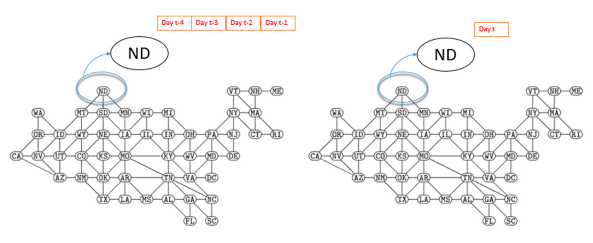
3.1. Graph Theory
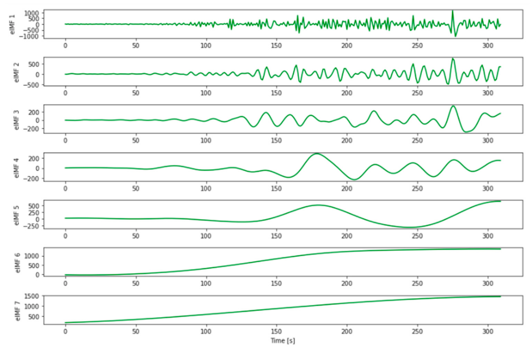
- Identification of all extreme values of x(t).
- Interpolation between all local maxima and minima to create upper and lower envelopes, i.e., emax(t) and emin(t).
- Computation of the average of these envelope values using the equation m(t) = [emax(t) + emin(t)]/2.
- Extraction of details using the equation h(t) = x(t) − m(t),
- Iteration on the residual r(t) = x(t) − c(t).
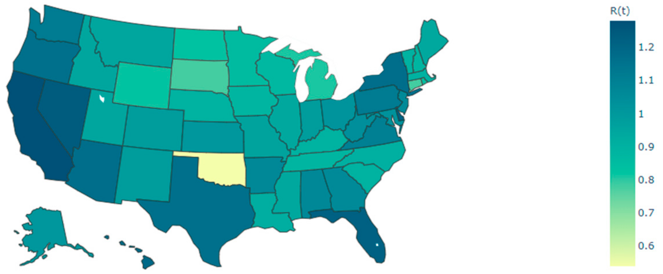
3.2. Effective Reproduction Number (Rt)
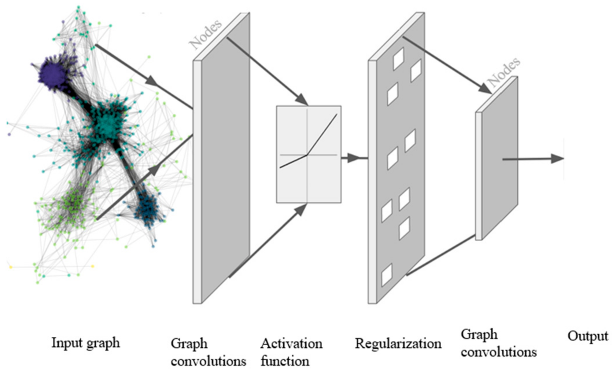
3.3. Graph Neural Networks (GNNs)
4. The Pandemic Prediction Model
5. Experimental Study
5.1. Experimental Design
5.2. Performance Metrics
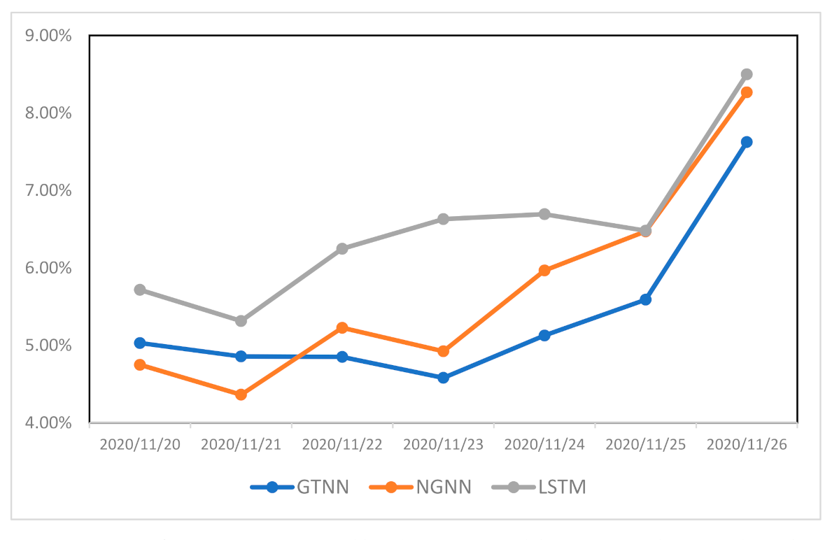
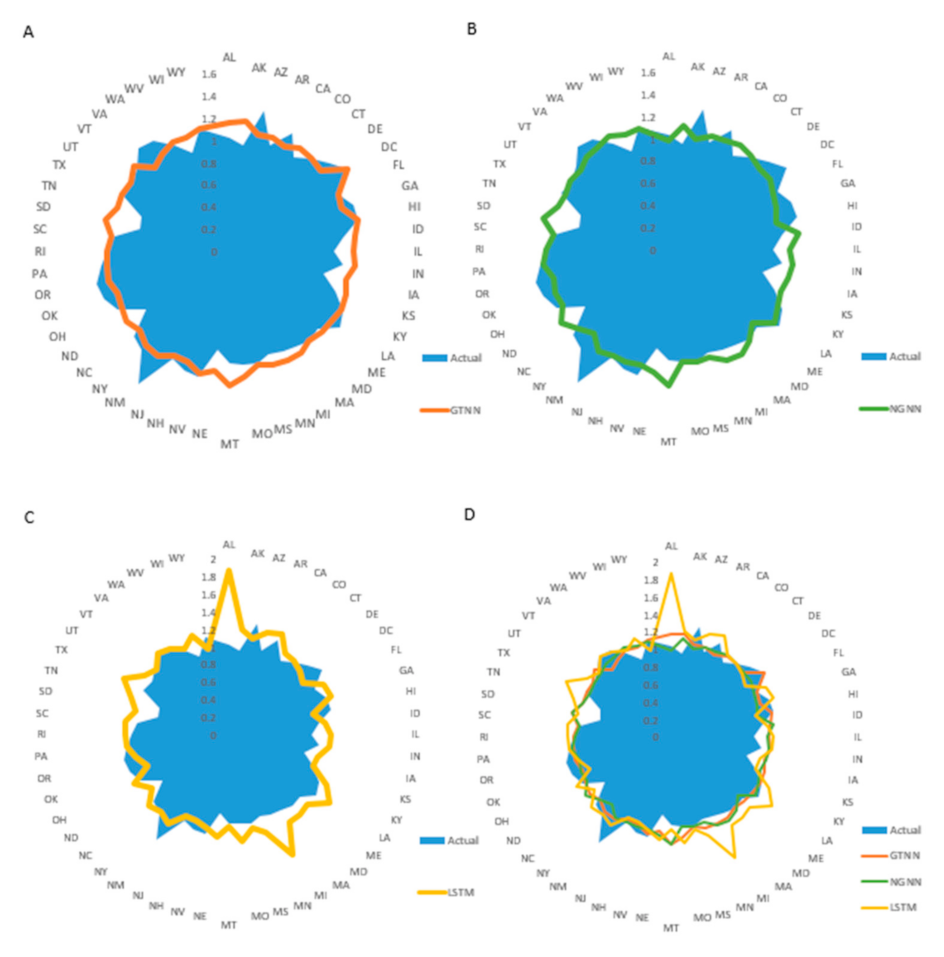
5.3. Performance Results
6. Limitations
7. Conclusions
Author Contributions
Funding
Institutional Review Board Statement
Informed Consent Statement
Data Availability Statement
Conflicts of Interest
References
- Bakar, N.A.; Rosbi, S. Effect of Coronavirus Disease (COVID-19) to Tourism Industry. Int. J. Adv. Eng. Res. Sci. 2020, 7, 189–193. [Google Scholar] [CrossRef] [Green Version]
- Davahli, M.R.; Karwowski, W.; Sonmez, S.; Apostolopoulos, Y. The Hospitality Industry in the Face of the COVID-19 Pandemic: Current Topics and Research Methods. Int. J. Environ. Res. Public. Health 2020, 17, 7366. [Google Scholar] [CrossRef] [PubMed]
- Gostic, K.M.; McGough, L.; Baskerville, E.B.; Abbott, S.; Joshi, K.; Tedijanto, C.; Kahn, R.; Niehus, R.; Hay, J.A.; Salazar, P.M.D.; et al. Practical Considerations for Measuring the Effective Reproductive Number, Rt. PLoS Comput. Biol. 2020, 16, e1008409. [Google Scholar] [CrossRef] [PubMed]
- Cori, A.; Ferguson, N.M.; Fraser, C.; Cauchemez, S. A New Framework and Software to Estimate Time-Varying Reproduction Numbers During Epidemics. Am. J. Epidemiol. 2013, 178, 1505–1512. [Google Scholar] [CrossRef] [Green Version]
- Sharma, N. Introduction to Graph Neural Networks. Available online: https://heartbeat.fritz.ai/introduction-to-graph-neural-networks-c5a9f4aa9e99 (accessed on 4 February 2021).
- CDC COVID-19 Cases, Deaths, and Trends in the US|CDC COVID Data Tracker. Available online: https://covid.cdc.gov/covid-data-tracker (accessed on 14 December 2020).
- Lalmuanawma, S.; Hussain, J.; Chhakchhuak, L. Applications of Machine Learning and Artificial Intelligence for Covid-19 (SARS-CoV-2) Pandemic: A Review. Chaos Solitons Fractals 2020, 139, 110059. [Google Scholar] [CrossRef]
- Zheng, Y.; Li, Z.; Xin, J.; Zhou, G. A Spatial-Temporal Graph Based Hybrid Infectious Disease Model with Application to COVID-19. arXiv 2020, arXiv:2010.09077. [Google Scholar]
- Nandini, G.K.; Rajan, R.S.; Shantrinal, A.A.; Rajalaxmi, T.M.; Rajasingh, I.; Balasubramanian, K. Topological and Thermodynamic Entropy Measures for COVID-19 Pandemic through Graph Theory. Symmetry 2020, 12, 1992. [Google Scholar] [CrossRef]
- Panagopoulos, G.; Nikolentzos, G.; Vazirgiannis, M. Transfer Graph Neural Networks for Pandemic Forecasting. arXiv 2020, arXiv:2009.08388v3. [Google Scholar]
- Cao, D.; Wang, Y.; Duan, J.; Zhang, C.; Zhu, X.; Huang, C.; Tong, Y.; Xu, B.; Bai, J.; Tong, J. Spectral Temporal Graph Neural Network for Multivariate Time-Series Forecasting. In Proceedings of the Conference on Neural Information Processing Systems, Vancouver, BC, Canada, 6–14 December 2020; Volume 33. [Google Scholar]
- La Gatta, V.; Moscato, V.; Postiglione, M.; Sperli, G. An Epidemiological Neural Network Exploiting Dynamic Graph Structured Data Applied to the COVID-19 Outbreak. IEEE Trans. Big Data 2020, 7, 45–55. [Google Scholar] [CrossRef]
- Kapoor, A.; Ben, X.; Liu, L.; Perozzi, B.; Barnes, M.; Blais, M.; O’Banion, S. Examining Covid-19 Forecasting Using Spatio-Temporal Graph Neural Networks. arXiv 2020, arXiv:200703113. [Google Scholar]
- Shah, C.; Dehmamy, N.; Perra, N.; Chinazzi, M.; Barabási, A.-L.; Vespignani, A.; Yu, R. Finding Patient Zero: Learning Contagion Source with Graph Neural Networks. arXiv 2020, arXiv:200611913. [Google Scholar]
- Farahani, F.V.; Karwowski, W.; Lighthall, N.R. Application of Graph Theory for Identifying Connectivity Patterns in Human Brain Networks: A Systematic Review. Front. Neurosci. 2019, 13, 585. [Google Scholar] [CrossRef]
- Cummings, D.A.; Irizarry, R.A.; Huang, N.E.; Endy, T.P.; Nisalak, A.; Ungchusak, K.; Burke, D.S. Travelling Waves in the Occurrence of Dengue Haemorrhagic Fever in Thailand. Nature 2004, 427, 344–347. [Google Scholar] [CrossRef]
- Flandrin, P.; Rilling, G.; Goncalves, P. Empirical Mode Decomposition as a Filter Bank. IEEE Signal Process. Lett. 2004, 11, 112–114. [Google Scholar] [CrossRef] [Green Version]
- Ismail, L.E.; Karwowski, W. A Graph Theory-Based Modeling of Functional Brain Connectivity Based on EEG: A Systematic Review in the Context of Neuroergonomics. IEEE Access 2020, 8, 155103–155135. [Google Scholar] [CrossRef]
- Sciré, J.; Nadeau, S.A.; Vaughan, T.G.; Gavin, B.; Fuchs, S.; Sommer, J.; Koch, K.N.; Misteli, R.; Mundorff, L.; Götz, T. Reproductive Number of the COVID-19 Epidemic in Switzerland with a Focus on the Cantons of Basel-Stadt and Basel-Landschaft. Swiss Med. Wkly. 2020, 150, w20271. [Google Scholar]
- Kenah, E.; Lipsitch, M.; Robins, J.M. Generation Interval Contraction and Epidemic Data Analysis. Math. Biosci. 2008, 213, 71–79. [Google Scholar] [CrossRef] [Green Version]
- Nishiura, H.; Linton, N.M.; Akhmetzhanov, A.R. Serial Interval of Novel Coronavirus (COVID-19) Infections. Int. J. Infect. Dis. 2020, 93, 284–286. [Google Scholar] [CrossRef]
- Kipf, T.N.; Welling, M. Semi-Supervised Classification with Graph Convolutional Networks. arXiv 2016, arXiv:160902907. [Google Scholar]
- Laszuk, D. EMD-Signal: Implementation of the Empirical Mode Decomposition (EMD) and Its Variations. Available online: https://github.com/laszukdawid/PyEMD (accessed on 10 March 2021).
- Paszke, A.; Gross, S.; Massa, F.; Lerer, A.; Bradbury, J.; Chanan, G.; Killeen, T.; Lin, Z.; Gimelshein, N.; Antiga, L. Pytorch: An Imperative Style, High-Performance Deep Learning Library. arXiv 2019, arXiv:191201703. [Google Scholar]
- Fey, M.; Lenssen, J.E. Fast Graph Representation Learning with PyTorch Geometric. arXiv 2019, arXiv:190302428. [Google Scholar]
- Kingma, D.P.; Ba, J. Adam: A Method for Stochastic Optimization. arXiv 2014, arXiv:14126980. [Google Scholar]
- De Myttenaere, A.; Golden, B.; Le Grand, B.; Rossi, F. Mean Absolute Percentage Error for Regression Models. Neurocomputing 2016, 192, 38–48. [Google Scholar] [CrossRef] [Green Version]
- Xu, J.; Rahmatizadeh, R.; Bölöni, L.; Turgut, D. Real-Time Prediction of Taxi Demand Using Recurrent Neural Networks. IEEE Trans. Intell. Transp. Syst. 2017, 19, 2572–2581. [Google Scholar] [CrossRef]


Publisher’s Note: MDPI stays neutral with regard to jurisdictional claims in published maps and institutional affiliations. |
© 2021 by the authors. Licensee MDPI, Basel, Switzerland. This article is an open access article distributed under the terms and conditions of the Creative Commons Attribution (CC BY) license (https://creativecommons.org/licenses/by/4.0/).
Share and Cite
Davahli, M.R.; Fiok, K.; Karwowski, W.; Aljuaid, A.M.; Taiar, R. Predicting the Dynamics of the COVID-19 Pandemic in the United States Using Graph Theory-Based Neural Networks. Int. J. Environ. Res. Public Health 2021, 18, 3834. https://0-doi-org.brum.beds.ac.uk/10.3390/ijerph18073834
Davahli MR, Fiok K, Karwowski W, Aljuaid AM, Taiar R. Predicting the Dynamics of the COVID-19 Pandemic in the United States Using Graph Theory-Based Neural Networks. International Journal of Environmental Research and Public Health. 2021; 18(7):3834. https://0-doi-org.brum.beds.ac.uk/10.3390/ijerph18073834
Chicago/Turabian StyleDavahli, Mohammad Reza, Krzysztof Fiok, Waldemar Karwowski, Awad M. Aljuaid, and Redha Taiar. 2021. "Predicting the Dynamics of the COVID-19 Pandemic in the United States Using Graph Theory-Based Neural Networks" International Journal of Environmental Research and Public Health 18, no. 7: 3834. https://0-doi-org.brum.beds.ac.uk/10.3390/ijerph18073834