
How Does Public Health Investment Affect Subjective Well-Being? Empirical Evidence from China

Abstract
:1. Introduction
1.1. Background
1.2. Literature Review
1.3. Theoretical Analysis
2. Materials and Methods
2.1. Data and Methodology
2.2. Model
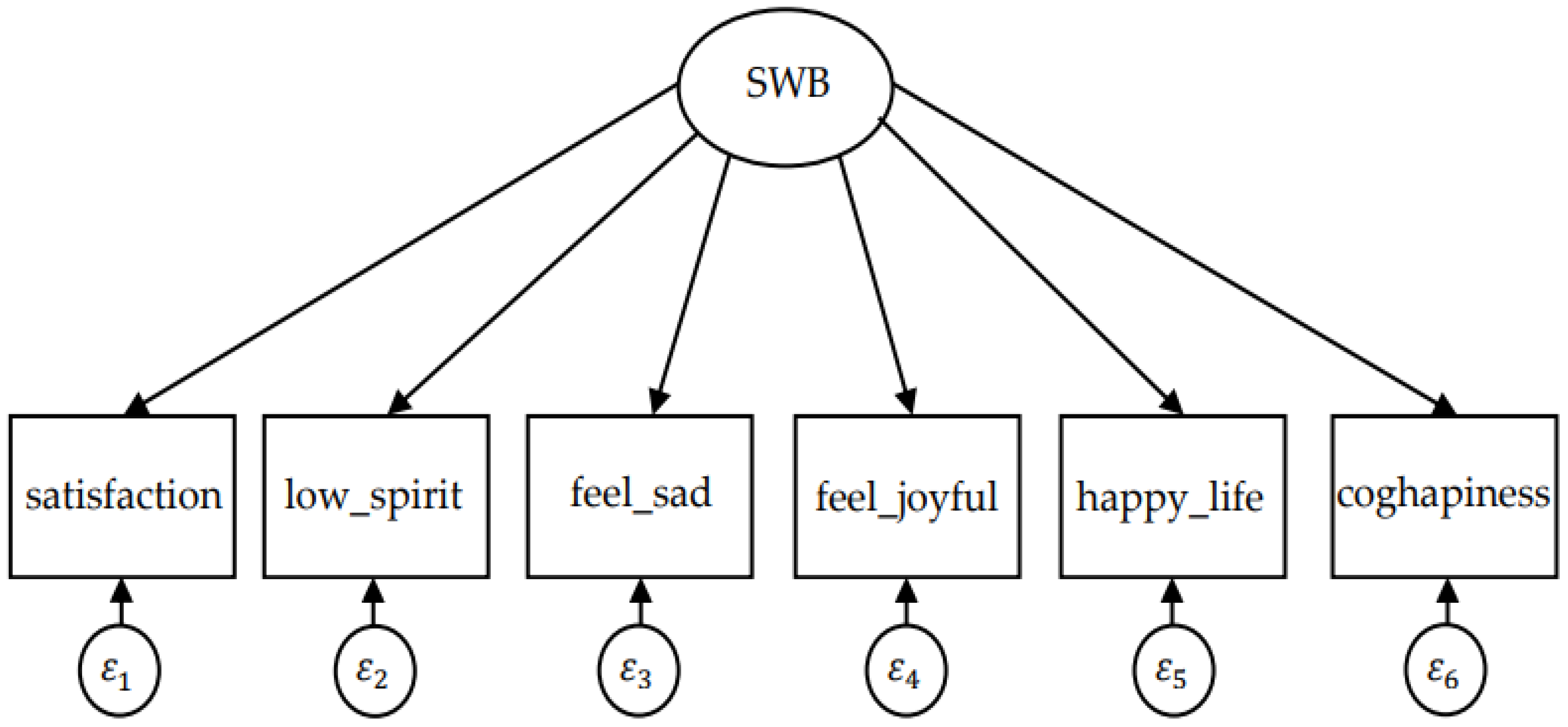
2.2.1. Factor Model
2.2.2. MIMIC Model
3. Results
3.1. Measuring Result of Factor Model
3.1.1. Exploratory Factor Analysis
3.1.2. Confirmatory Factor Analysis
3.2. Measured Value of Subjective Well-Being
3.3. Estimation Results of Basic MIMIC Model
3.4. Further Heterogeneity Analysis
4. Discussion
4.1. Results Analysis and Policy Implication
4.2. Limitations
5. Conclusions
Author Contributions
Funding
Institutional Review Board Statement
Informed Consent Statement
Data Availability Statement
Conflicts of Interest
References
- Manioudis, M.; Meramveliotakis, G. Broad strokes towards a grand theory in the analysis of sustainable development: A return to the classical political economy. New Political Econ. 2022, 1–13. [Google Scholar] [CrossRef]
- Jackson, T.; Marks, N. Consumption, sustainable welfare and human needs—With reference to UK expenditure patterns between 1954 and 1994. Ecol. Econ. 1999, 28, 421–441. [Google Scholar] [CrossRef]
- Gatersleben, B. Sustainable household consumption and quality of life: The acceptability of sustainable consumption patterns and consumer policy strategies. International. Int. J. Environ. Pollut. 2001, 15, 200–216. [Google Scholar] [CrossRef] [Green Version]
- Rinne, J.; Lyytimaeki, J.; Kautto, P. From sustainability to well-being: Lessons learned from the use of sustainable development indicators at national and EU level. Ecol. Indic. 2013, 35, 35–42. [Google Scholar] [CrossRef]
- Munro, L.T. where did bhutan’s gross national happiness come from? The origins of an invented tradition. Asian Aff. 2016, 47, 71–92. [Google Scholar] [CrossRef]
- Diener, E. Subjective well-being. The science of happiness and a proposal for a national index. Am. Psychol. 2000, 55, 34–43. [Google Scholar] [CrossRef]
- Layard, R. Happiness: Lessons from A New Science. Foreign Aff. 2005, 84, 416–425. [Google Scholar]
- Diener, E.; Seligman, M. Beyond Money: Toward an Economy of Well-Being. Psychol. Sci. Public Interest 2004, 5, 1–31. [Google Scholar] [CrossRef]
- Easterlin, R.A. Does Money Buy Happiness? Public Interest 1973, 30, 3–10. [Google Scholar]
- Frey, B.S.; Stutzer, A. Happiness, economy and institutions. Econ. J. 2000, 110, 918–938. [Google Scholar] [CrossRef]
- Wolfers, J. Is business cycle volatility costly? Evidence from surveys of subjective wellbeing. Int. Financ. 2003, 6, 1–26. [Google Scholar] [CrossRef]
- Zimmermann, A.C.; Easterlin, R.A. Happily Ever After? Cohabitation, Marriage, Divorce, and Happiness in Germany. Popul. Dev. Rev. 2006, 32, 1–24. [Google Scholar] [CrossRef]
- Levinson, A. Valuing Public Goods Using Happiness Data: The Case of Air Quality. J. Public Econ. 2012, 96, 869–880. [Google Scholar] [CrossRef]
- Layard, R. Happiness and Public Policy: A Challenge to the Profession. Econ. J. 2006, 116, 24–33. [Google Scholar] [CrossRef]
- Clark, A.E.; Frijters, P.; Shields, M. Relative Income, Happines, and Utility: An Explanation for the Easterlin Paradox and Other Puzzles. J. Econ. Lit. 2008, 46, 95–144. [Google Scholar] [CrossRef] [Green Version]
- Knight, J.; Gunatilaka, R. Does Economic Growth Raise Happiness in China? Oxf. Dev. Stud. 2011, 39, 1–24. [Google Scholar] [CrossRef]
- Deaton, A. What Do Self-reports of Wellbeing Say about Life-cycle Theory and Policy? J. Public Econ. 2018, 162, 18–25. [Google Scholar] [CrossRef]
- Klein, C. Social Capital or Social Cohesion: What Matters for Subjective Well-Being? Soc. Indic. Res. 2013, 110, 891–911. [Google Scholar] [CrossRef]
- Diener, E.; Suh, M.E. Subjective well-being and age: An international analysis. Annu. Rev. Gerontol. Geriatr. 1997, 17, 304–324. [Google Scholar]
- Hayo, B. Happiness in Eastern Europe; Marburg Working Papers on Economics: Marburg, Germany, 2004. [Google Scholar]
- Alesina, A.F.; Tella, R.D.; MacCulloch, R. Inequality and Happiness: Are Europeans and Americans Different? J. Public Econ. 2004, 88, 2009–2042. [Google Scholar] [CrossRef] [Green Version]
- Graham, C.; Felton, A. Inequality and happiness: Insights from Latin America. J. Econ. Inequal. 2006, 4, 107–122. [Google Scholar] [CrossRef]
- Grover, S.; Helliwell, J.F. How’s Life at Home? New Evidence on Marriage and the Set Point for Happiness. J. Happiness Stud. 2019, 20, 373–390. [Google Scholar] [CrossRef] [Green Version]
- Blanchflower, D.; Oswald, A. Well-being over time in Britain and the USA. J. Public Econ. 2004, 88, 1359–1386. [Google Scholar] [CrossRef] [Green Version]
- Oreopoulos, P. Do dropouts drop out too soon? Wealth, health and happiness from compulsory schooling. J. Public Econ. 2007, 91, 2213–2229. [Google Scholar] [CrossRef]
- Weisbach, D.A. The Taxation of Carried Interests in Private Equity. Va Law Rev. 2008, 94, 715–764. [Google Scholar]
- Clark, A.E.; Oswald, A.J. Subjective well-being and unemployment. Econ. J. 1994, 104, 648–659. [Google Scholar] [CrossRef]
- Helliwell, J.F.; Putnam, R.D. The social context of well-being. Philos. T. R. Soc. B 2004, 359, 1435–1446. [Google Scholar] [CrossRef]
- Tella, R.D.; Macculloch, R.J.; Oswald, A.J. The Macroeconomics of Happiness. Rev. Econ. Stat. 2003, 85, 809–827. [Google Scholar] [CrossRef] [Green Version]
- Yew-Kwang, N.G. From preference to happiness: Towards a more complete welfare economics. Soc. Choice Welf. 2003, 20, 307–350. [Google Scholar]
- Oishi, S.; Graham, J.; Kesebir, S.; Galinha, I.C. Concepts of happiness across time and cultures. Pers. Soc. Psychol. Bull. 2013, 39, 559–577. [Google Scholar] [CrossRef]
- Hu, H.S.; Lu, Y.P. Public Expenditure and Subjective Well-being of Rural Citizens—An Empirical Analysis Based on CGSS Data. Financ. Trade Econ. 2012, 10, 23–33. (In Chinese) [Google Scholar]
- Bjrnskov, C.; Dreher, A.; Fischer, J. The Bigger the Better? Evidence of the Effect of Government Size on Life Satisfaction around the World. Public Choice 2005, 130, 267–292. [Google Scholar] [CrossRef] [Green Version]
- Dutt, A. Consumption and Happiness: Alternative Approaches; University of Note Dame: South Bend, IN, USA, 2006; pp. 1–58. [Google Scholar]
- Helliwell, J.F.; Haifang, H. How’s Your Government? International Evidence Linking Good Government and Well-Being. Br. J. Polit. Sci. 2008, 38, 595–620. [Google Scholar] [CrossRef] [Green Version]
- Kotakorpi, K.; Laamanen, J.P. Welfare State and Life Satisfaction: Evidence from Public Health Care. Economica 2010, 77, 565–583. [Google Scholar] [CrossRef] [Green Version]
- Lu, Y.P.; Zhang, K.Z. Economic growth, pro-poor spending and national happiness—Empirical study based on China’s well-being data. Economist 2010, 10, 5–14. (In Chinese) [Google Scholar]
- Hessami, Z. The Size and Composition of Government Spending in Europe and Its Impact on Well-Being; MPRA Paper; University Library of Munich: Munich, Germany, 2010; Volume 63, pp. 346–382. [Google Scholar]
- Lok-Sang, H.O.; Yew-Kwang, N.G. Happiness and Government: The Role of Public Spending and Public Governance; CPPS Working Papers: Hongkong, China, 2016. [Google Scholar]
- Tang, F.L.; Lei, P.F. Income gap, residents’ happiness and public expenditure policy—Empirical analysis based on the Chinese Social Comprehensive Survey. Econ. Perspect. 2014, 10, 41–55. (In Chinese) [Google Scholar]
- Welsch, H.; Kühling, J. Are pro-environmental consumption choices utility-maximizing? Evidence from subjective well-being data. Ecol. Econ. 2011, 72, 75–87. [Google Scholar] [CrossRef]
- Veenhoven, R.; Ehrhardt, J. The cross-national pattern of happiness: Test of predictions implied in three theories of happiness. Soc. Indic. Res. 1995, 34, 33–68. [Google Scholar] [CrossRef] [Green Version]
- Xie, Y.; Lu, P. The sampling design of the China Family Panel Studies (CFPS). Chin. J. Sociol. 2015, 1, 471–484. [Google Scholar] [CrossRef]
- Dolan, P.; Peasgood, T.; White, M. Do we really know what makes us happy? A review of the economic literature on the factors associated with subjective well -being. J. Econ. Psychol. 2008, 29, 94–122. [Google Scholar] [CrossRef]
- Kimball, M.S.; Nunn, R.; Silverman, D. Accounting for Adaptation in the Economics of Happiness; NBER Working Paper: Cambridge, MA, USA, 2015; Volume 6. [Google Scholar]
- Lohmann, S. Information Technologies and Subjective Well-being: Does the Internet Raise Material Aspirations? Oxf. Econ. Pap. 2015, 67, 740–759. [Google Scholar] [CrossRef] [Green Version]
- Acock, A. Discovering Structural Equation Modeling Using Stata; Stata Press: College Station, TX, USA, 2013. [Google Scholar]
- Schumacker, R.E.; Lomax, R.G. Beginner’s Guide to Structural Equation Modeling; Lawewnce Erlbaum Associates: Mahwah, NJ, USA, 2004. [Google Scholar]
- Hawkes, N. Happiness is U shaped, highest in the teens and 70s, survey shows. Br. Med. J. 2012, 344, 1. [Google Scholar] [CrossRef] [PubMed]
- Burr, A.; Santo, J.B.; Pushkar, D. Affective Well-Being in Retirement: The Influence of Values, Money, and Health across Three Years. J. Happiness Stud. 2011, 12, 17–40. [Google Scholar] [CrossRef] [Green Version]
- Anderson, C.; John, O.P.; Keltner, D. Who Attains Social Status? Effects of Personality and Physical Attractiveness in Social Groups. J. Pers. Soc. Psychol. 2001, 81, 116–132. [Google Scholar] [CrossRef]
- Ram, R. Government Spending and Happiness of the Population: Additional Evidence from Large Cross-Country Samples. Public Choice 2009, 138, 483–490. [Google Scholar] [CrossRef]
- Kim, S.; Kim, D. Does Government Make People Happy? Exploring New Research Directions for Government’s Roles in Happiness. J. Happiness Stud. 2012, 40, 1190–1200. [Google Scholar] [CrossRef]


| Variable Name | Label | Description | ||
|---|---|---|---|---|
| Subjective Well-being (SWB) | Life satisfaction | satisfaction | Are you satisfied with your life? | 1–5 denotes from very unsatisfied to very satisfied |
| Positive emotions | posemotion | I feel joyful | 1 = Never (less than one day) 2 = Sometimes (1–2 days) 3 = Often (3–4 days) 4 = Most of the time (5–7 days) | |
| I have a happy life | ||||
| Negative emotions | negemotion | I am in a low spirit | 1 = Most of the time (5–7 days) 2 = Often (3–4 days) 3 = Sometimes (1–2 days) 4 = Never (less than one day) | |
| I feel sad | ||||
| Overall cognitive happiness valuation | coghapiness | How happy are you? (score) | 0–10 denotes from very unhappy to very happy | |
| Public health investment | phe | Per capita public health investment | ||
| The disparity of public health investment | disparity | Individual relative deprivation index of public health investment | ||
| Age | age | Age of respondents | ||
| Gender | gender | 1 = man; 0 = woman | ||
| Ethnicity | ethnicity | 1 = Han; 0 = another minority | ||
| Marital status | marry | 1 = in marriage; 0 = not in marriage | ||
| Education | education | Years of schooling | ||
| Registered permanent residence | identity | 1 = rural; 0 = urban | ||
| Relative income | income | 1–5 denotes from very low-income level to a very high-income level in local | ||
| Health status | health | 1 = Excellent; 2 = Very good; 3 = Good; 4 = Fair; 5 = Poor | ||
| Social status | status | 1–5 denotes from very low to very high in local | ||
| Politics status | party | 1 = a member of Communist Party of China; 0 = not a member of Communist Party of China | ||
| Household income level | lnphinc | The logarithm of per capita household income | ||
| Family relationships | family | How many times do you usually have dinner with your family in one week | ||
| Social network | lngift | The logarithm of gift expenditure | ||
| Variable Label | Mean | S.D. | Min | Median | Max |
|---|---|---|---|---|---|
| satisfaction | 4.040 | 0.950 | 1 | 4 | 5 |
| low_spirit | 3.270 | 0.760 | 1 | 3 | 4 |
| feel_sad | 3.490 | 0.700 | 1 | 4 | 4 |
| feel_joyful | 2.900 | 0.930 | 1 | 3 | 4 |
| happy_life | 3.050 | 0.900 | 1 | 3 | 4 |
| coghapiness | 7.540 | 2.110 | 1 | 8 | 10 |
| phe | 1021 | 231.5 | 770.5 | 1002 | 2782 |
| disparity | 0.120 | 0.0500 | 0 | 0.110 | 0.210 |
| age | 47.89 | 15.32 | 16 | 48 | 96 |
| gender | 0.490 | 0.500 | 0 | 0 | 1 |
| ethnicity | 0.910 | 0.290 | 0 | 1 | 1 |
| marry | 0.870 | 0.340 | 0 | 1 | 1 |
| education | 7.630 | 4.960 | 0 | 9 | 22 |
| identity | 0.730 | 0.440 | 0 | 1 | 1 |
| income | 2.930 | 1.070 | 1 | 3 | 5 |
| health | 3.060 | 1.210 | 1 | 3 | 5 |
| status | 3.130 | 1.070 | 1 | 3 | 5 |
| party | 0.100 | 0.300 | 0 | 0 | 1 |
| lnphinc | 9.390 | 1.010 | 0.920 | 9.430 | 13.30 |
| family | 5.850 | 2.230 | 0 | 7 | 7 |
| lngift | 8 | 1.040 | 1.610 | 8.010 | 11.98 |
| Variable Label | Frequency | Percent | Cumulative Distribution |
|---|---|---|---|
| satisfaction | |||
| 1 | 416 | 1.81 | 1.81 |
| 2 | 675 | 2.93 | 4.74 |
| 3 | 5391 | 23.41 | 28.14 |
| 4 | 7644 | 33.19 | 61.33 |
| 5 | 8905 | 38.67 | 100 |
| feel_joyful | |||
| 1 | 1681 | 7.3 | 7.3 |
| 2 | 6064 | 26.33 | 33.63 |
| 3 | 8082 | 35.09 | 68.72 |
| 4 | 7204 | 31.28 | 100 |
| happy_life | |||
| 1 | 1336 | 5.8 | 5.8 |
| 2 | 4820 | 20.93 | 26.73 |
| 3 | 8230 | 35.73 | 62.46 |
| 4 | 8645 | 37.54 | 100 |
| low_spirit | |||
| 1 | 834 | 3.62 | 3.62 |
| 2 | 1862 | 8.08 | 11.71 |
| 3 | 10,682 | 46.38 | 58.09 |
| 4 | 9653 | 41.91 | 100 |
| feel_sad | |||
| 1 | 565 | 2.45 | 2.45 |
| 2 | 999 | 4.34 | 6.79 |
| 3 | 8072 | 35.05 | 41.84 |
| 4 | 13,395 | 58.16 | 100 |
| coghapiness | |||
| 1 | 297 | 1.29 | 1.29 |
| 2 | 190 | 0.82 | 2.11 |
| 3 | 444 | 1.93 | 4.04 |
| 4 | 439 | 1.91 | 5.95 |
| 5 | 3609 | 15.67 | 21.62 |
| 6 | 1856 | 8.06 | 29.68 |
| 7 | 2461 | 10.69 | 40.36 |
| 8 | 5954 | 25.85 | 66.22 |
| 9 | 1850 | 8.03 | 74.25 |
| 10 | 5931 | 25.75 | 100 |
| Factor | Principal Axis Factor Method (PF) | Iterative Principal Axis Factor Method (IPF) | Maximum Likelihood Factor Method (MLF) |
|---|---|---|---|
| Factor 1 | 1.74 | 1.97 | 1.86 |
| Factor 2 | 0.32 | 0.54 | 0.54 |
| Factor 3 | 0.26 | 0.49 | — |
| Factor 4 | −0.19 | 0.03 | — |
| Factor 5 | −0.21 | 0.01 | — |
| Factor 6 | −0.22 | −0.0002 | — |
| Indicator | CFI | R2(CD) | RMSEA |
|---|---|---|---|
| Test result | 0.999 | 0.596 | 0.016 |
| judgement criteria | above 0.90 | below 0.08 |
| Region | Value Adjustment Factor | Standardized Value | Region | Value Adjustment Factor | Standardized Value |
|---|---|---|---|---|---|
| Beijing | 11.97 | 89.58 | Shandong | 12.31 | 90.67 |
| Tianjin | 12.13 | 90.10 | Henan | 11.99 | 89.65 |
| Hebei | 12.02 | 89.74 | Hubei | 11.97 | 89.57 |
| Shanxi | 11.71 | 88.71 | Hunan | 11.76 | 88.89 |
| Liaoning | 12.14 | 90.11 | Guangdong | 11.40 | 87.71 |
| Jilin | 11.84 | 89.15 | Guangxi | 11.14 | 86.85 |
| Heilongjiang | 12.12 | 90.05 | Chongqing | 11.51 | 88.08 |
| Shanghai | 12.19 | 90.30 | Sichuan | 11.88 | 89.27 |
| Jiangsu | 12.02 | 89.73 | Guizhou | 10.91 | 86.11 |
| Zhejiang | 12.06 | 89.88 | Yunnan | 11.47 | 87.93 |
| Anhui | 11.94 | 89.47 | Shanxi | 11.22 | 87.12 |
| Fujian | 11.10 | 86.72 | Gansu | 11.32 | 87.44 |
| Jiangxi | 11.20 | 87.06 | average | 11.76 | 89.09 |
| Variable | (1) | (2) | (3) |
|---|---|---|---|
| ML | ML + Robust | MLMV + Robust | |
| A. Structural Equation | |||
| phe | 0.0007 *** | 0.0007 *** | 0.0006 *** |
| (8.74) | (8.71) | (8.14) | |
| disparity | 8.1965 *** | 8.1965 *** | 7.2559 *** |
| (7.43) | (7.41) | (6.89) | |
| disparity2 | −17.1280 *** | −17.1280 *** | −14.6824 *** |
| (−5.35) | (−5.34) | (−4.79) | |
| age | −0.0152 *** | −0.0152 *** | −0.0180 *** |
| (−9.12) | (−8.54) | (−10.90) | |
| age2 | 0.0002 *** | 0.0002 *** | 0.0002 *** |
| (11.94) | (11.04) | (13.53) | |
| gender | 0.0439 *** | 0.0439 *** | 0.0325 *** |
| (5.50) | (5.29) | (4.07) | |
| ethnicity | −0.0332 ** | −0.0332 ** | −0.0116 |
| (−2.45) | (−2.39) | (−0.88) | |
| marry | 0.1456 *** | 0.1456 *** | 0.2002 *** |
| (11.31) | (10.26) | (15.95) | |
| education | 0.0030 *** | 0.0030 *** | 0.0036 *** |
| (2.81) | (2.65) | (3.37) | |
| identity | −0.0634 *** | −0.0634 *** | −0.0742 *** |
| (−6.22) | (−6.32) | (−7.75) | |
| income | 0.0817 *** | 0.0817 *** | 0.0828 *** |
| (17.39) | (13.76) | (14.78) | |
| health | −0.1406 *** | −0.1406 *** | −0.1401 *** |
| (−36.74) | (−33.66) | (−35.85) | |
| status | 0.1030 *** | 0.1030 *** | 0.1110 *** |
| (20.95) | (15.70) | (17.37) | |
| party | 0.0069 | 0.0069 | 0.0162 |
| (0.52) | (0.55) | (1.35) | |
| lnphinc | 0.0568 *** | 0.0568 *** | 0.0486 *** |
| (12.33) | (11.80) | (11.29) | |
| family | 0.0204 *** | 0.0204 *** | 0.0208 *** |
| (11.31) | (11.06) | (11.26) | |
| lngift | 0.0138 *** | 0.0138 *** | 0.0176 *** |
| (3.51) | (3.49) | (4.50) | |
| B. Measurement Equation | |||
| satisfaction | 1.0000 | 1.0000 | 1.0000 |
| (.) | (.) | (.) | |
| low_spirit | 0.6065 *** | 0.6065 *** | 0.5736 *** |
| (35.27) | (25.45) | (26.48) | |
| feel_sad | 0.5855 *** | 0.5855 *** | 0.5713 *** |
| (34.32) | (22.82) | (23.77) | |
| feel_joyful | 0.8538 *** | 0.8538 *** | 0.8175 *** |
| (37.08) | (26.50) | (27.56) | |
| happy_life | 0.8814 *** | 0.8814 *** | 0.8597 *** |
| (38.25) | (27.36) | (28.51) | |
| coghapiness | 2.4346 *** | 2.4346 *** | 2.4311 *** |
| (53.09) | (40.95) | (44.13) | |
| C. Fit Index | |||
| N | 23,031 | 23,031 | 27,062 |
| RMSEA | 0.041 | ||
| CFI | 0.901 | ||
| SRMR | 0.026 | 0.026 | |
| R2(CD) | 0.367 | 0.367 | 0.367 |
| Variable | (1) | (2) | (3) | (4) | (5) |
|---|---|---|---|---|---|
| MLMV + Robust | |||||
| Low | Low–Middle | Middle | Upper Middle | High | |
| A. Structural Equation | |||||
| phe | 0.0006 *** | 0.0007 *** | 0.0005 *** | 0.0005 *** | 0.0003 *** |
| (4.43) | (3.07) | (2.81) | (3.42) | (2.67) | |
| disparity | 7.6012 *** | 9.0059 *** | 9.1372 *** | 5.6687 *** | 2.7784 |
| (4.73) | (3. 87) | (4.43) | (2.64) | (1.46) | |
| disparity2 | −14.8418 *** | −19.4051 *** | −23.0571 *** | −10.6304 * | −3.3760 |
| (−3.04) | (−2.78) | (−3.86) | (−1.69) | (−0.59) | |
| age | −0.0161 *** | −0.0203 *** | −0.0129 *** | −0.0162 *** | −0.0093 ** |
| (−5.17) | (−4.97) | (−3.55) | (−4.35) | (−2.50) | |
| age2 | 0.0002 *** | 0.0003 *** | 0.0002 *** | 0.0002 *** | 0.0001 *** |
| (6.29) | (6.16) | (5.25) | (5.68) | (3.85) | |
| gender | 0.0358 ** | 0.0707 *** | 0.0383 ** | 0.0612 *** | 0.0287 |
| (2.25) | (3.64) | (2.24) | (3.43) | (1.63) | |
| ethnicity | −0.0822 *** | −0.0296 | −0.0236 | −0.0030 | 0.0542 |
| (−3.56) | (−0.96) | (−0.75) | (−0.08) | (1.43) | |
| marry | 0.1440 *** | 0.1437 *** | 0.1523 *** | 0.1308 *** | 0.1794 *** |
| (5.96) | (4.50) | (5.47) | (4.39) | (6.13) | |
| education | 0.0061 *** | 0.0066 *** | 0.0026 | −0.0006 | −0.0026 |
| (3.00) | (2.58) | (1.12) | (−0.24) | (−1.02) | |
| identity | −0.1321 *** | −0.0102 | −0.0190 | −0.0822 *** | −0.0570 *** |
| (−5.19) | (−0.33) | (−0.93) | (−4.13) | (−2.73) | |
| income | 0.1035 *** | 0.0470 *** | 0.0802 *** | 0.0737 *** | 0.0894 *** |
| (12.78) | (4.71) | (8.50) | (7.09) | (7.99) | |
| health | −0.1318 *** | −0.1435 *** | −0.1513 *** | −0.1473 *** | −0.1259 *** |
| (−20.40) | (−17.50) | (−19.99) | (−17.69) | (−14.63) | |
| status | 0.1038 *** | 0.1035 *** | 0.0910 *** | 0.0992 *** | 0.1158 *** |
| (12.64) | (9.79) | (9.51) | (9.66) | (10.12) | |
| party | 0.0242 | −0.0107 | 0.0302 | −0.0146 | 0.0230 |
| (0.77) | (−0.27) | (1.01) | (−0.52) | (0.98) | |
| lnphinc | 0.0347 *** | 0.0427 | 0.0564 | 0.0679 * | 0.0618 *** |
| (4.06) | (0.91) | (1.47) | (1.86) | (3.31) | |
| lngift | 0.0218 *** | 0.0001 | −0.0057 | 0.0171 * | 0.0254 *** |
| (2.83) | (0.1) | (−0.67) | (1.92) | (2.78) | |
| family | 0.0147 *** | 0.0149 *** | 0.0218 *** | 0.0248 *** | 0.0268 *** |
| (3.93) | (3.30) | (5.95) | (6.30) | (6.67) | |
| N | 6574 | 3967 | 4572 | 4236 | 3682 |
| Variable | (1) | (2) | (3) | (4) |
|---|---|---|---|---|
| MLMV + Robust | ||||
| East | Midwest | Rural | Urban | |
| phe | 0.0005 *** | 0.0004 *** | 0.0006 *** | 0.0005 *** |
| (4.88) | (2.98) | (6.83) | (5.55) | |
| disparity | 6.4905 *** | 9.8656 *** | 8.2085 *** | 5.1556 *** |
| (3.89) | (7.19) | (7.2) | (3.9) | |
| disparity2 | −13.9285 *** | −26.3968 *** | −18.0201 *** | −8.3904 *** |
| (−2.83) | (−6.00) | (−5.38) | (−2.13) | |
| age | −0.0146 *** | −0.0150 *** | −0.0152 *** | −0.0119 *** |
| (−5.78) | (−7.00) | (−7.74) | (−3.98) | |
| age2 | 0.0002 *** | 0.0002 *** | 0.0002 *** | 0.0002 *** |
| (7.54) | (9.21) | (9.99) | (5.76) | |
| gender | 0.0649 *** | 0.0322 *** | 0.0417 *** | 0.0513 *** |
| (5.33) | (3.10) | (4.41) | (3.57) | |
| ethnicity | −0.0080 | −0.0607 *** | −0.0461 *** | 0.0088 |
| (−0.3) | (−3.72) | (−3.07) | (0.27) | |
| marry | 0.1856 *** | 0.1219 *** | 0.1454 *** | 0.1375 *** |
| (9.15) | (7.46) | (9.54) | (5.94) | |
| education | 0.0019 | 0.0031 *** | 0.0045 *** | −0.0009 |
| (1.13) | (2.30) | (3.6) | (−0.44) | |
| identity | −0.0682 *** | −0.0645 *** | - | - |
| (−4.5) | (−4.64) | - | - | |
| income | 0.0855 *** | 0.0790 *** | 0.0848 *** | 0.0673 *** |
| (12.12) | (13.77) | (16.06) | (7.78) | |
| health | −0.1406 *** | −0.1396 *** | −0.1403 *** | −0.1401 *** |
| (−25.09) | (−29.81) | (−32.95) | (−19.87) | |
| status | 0.1017 *** | 0.1036 *** | 0.0977 *** | 0.1182 *** |
| (14.15) | (17.29) | (17.85) | (13.35) | |
| party | 0.00007 | 0.0161 | 0.0175 | −0.0002 |
| (0.00) | (0.93) | (0.94) | (−0.01) | |
| lnphinc | 0.0601 *** | 0.0465 *** | 0.0572 *** | 0.0564 *** |
| (8.40) | (7.62) | (10.85) | (6.06) | |
| family | 0.0208 *** | 0.0196 *** | 0.0181 *** | 0.0270 *** |
| (7.56) | (8.37) | (8.61) | (8.03) | |
| lngift | 0.0084 | 0.0200 *** | 0.0058 | 0.0365 *** |
| (1.4) | (3.85) | (1.26) | (4.86) | |
| N | 9162 | 13,869 | 16,917 | 6114 |
Publisher’s Note: MDPI stays neutral with regard to jurisdictional claims in published maps and institutional affiliations. |
© 2022 by the authors. Licensee MDPI, Basel, Switzerland. This article is an open access article distributed under the terms and conditions of the Creative Commons Attribution (CC BY) license (https://creativecommons.org/licenses/by/4.0/).
Share and Cite
Yang, Y.; Zhao, L.; Cui, F. How Does Public Health Investment Affect Subjective Well-Being? Empirical Evidence from China. Int. J. Environ. Res. Public Health 2022, 19, 5035. https://0-doi-org.brum.beds.ac.uk/10.3390/ijerph19095035
Yang Y, Zhao L, Cui F. How Does Public Health Investment Affect Subjective Well-Being? Empirical Evidence from China. International Journal of Environmental Research and Public Health. 2022; 19(9):5035. https://0-doi-org.brum.beds.ac.uk/10.3390/ijerph19095035
Chicago/Turabian StyleYang, Yingzhu, Lexiang Zhao, and Feng Cui. 2022. "How Does Public Health Investment Affect Subjective Well-Being? Empirical Evidence from China" International Journal of Environmental Research and Public Health 19, no. 9: 5035. https://0-doi-org.brum.beds.ac.uk/10.3390/ijerph19095035