

Risk Assessment and Source Apportionment of Metals on Atmospheric Particulate Matter in a Suburban Background Area of Gran Canaria (Spain)


Abstract
:
1. Introduction
2. Materials and Methods
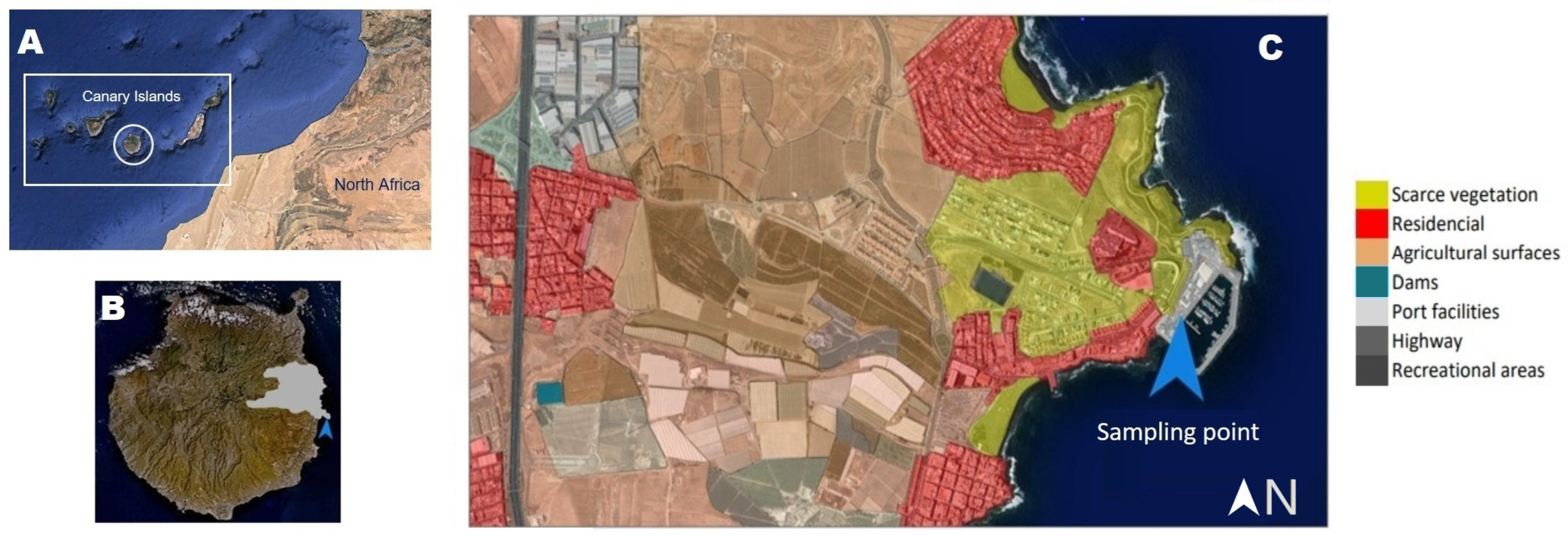
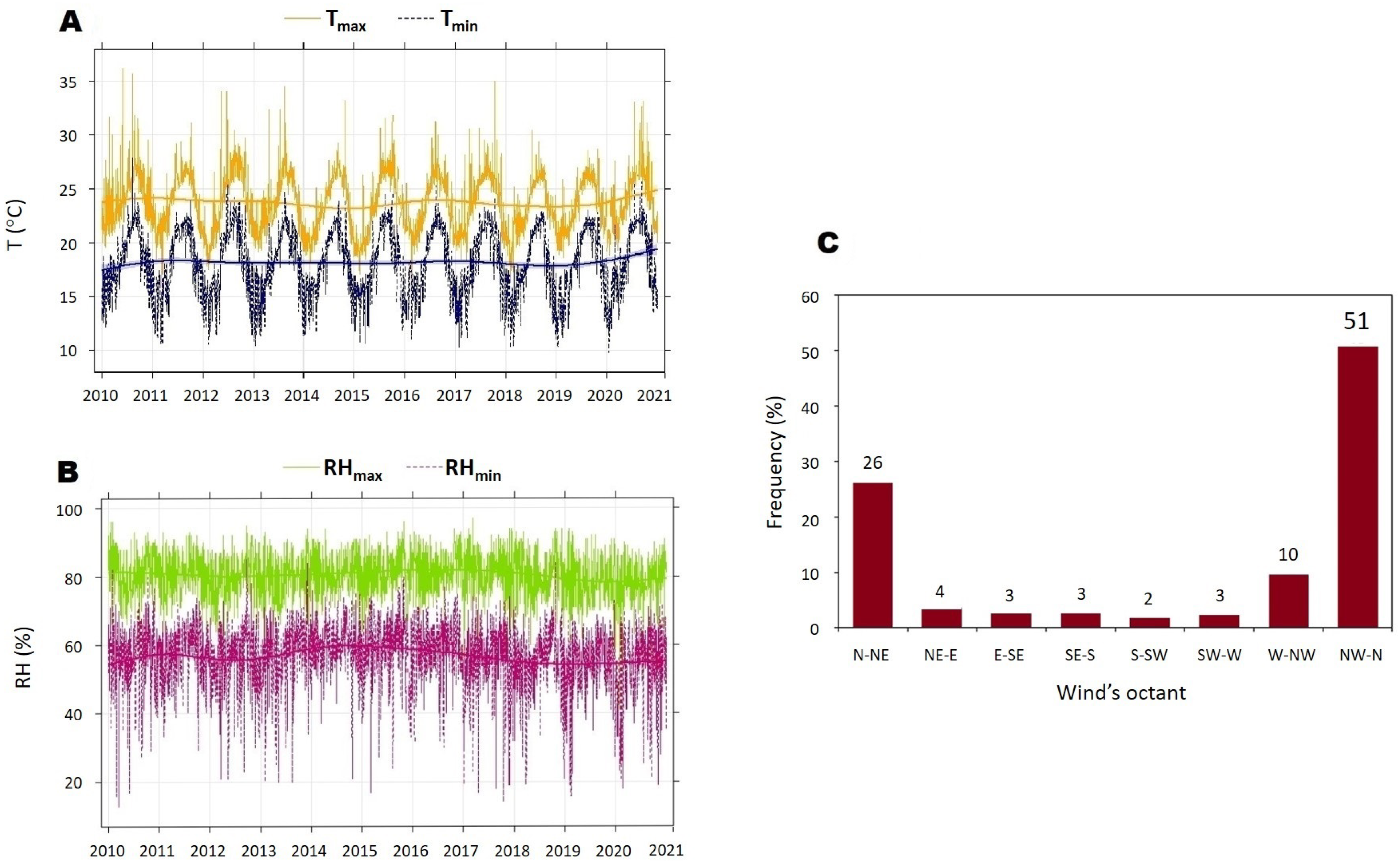
2.1. Area of Study
2.2. Sampling
2.3. Sample Treatment and Chemical Analysis
2.4. Health Risk Assessment
2.5. Source Apportionment
2.5.1. Enrichment Factors (EFs)
2.5.2. Positive Matrix Factorization (PMF)
3. Results and Discussion
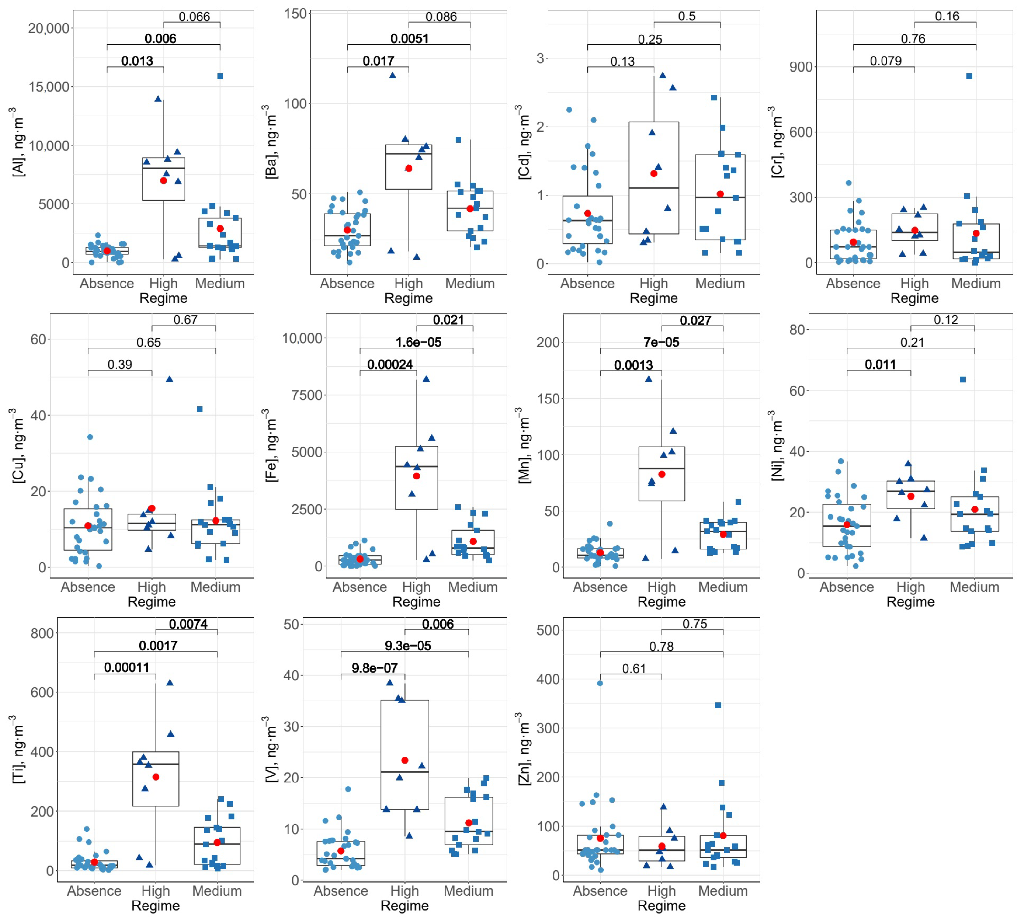
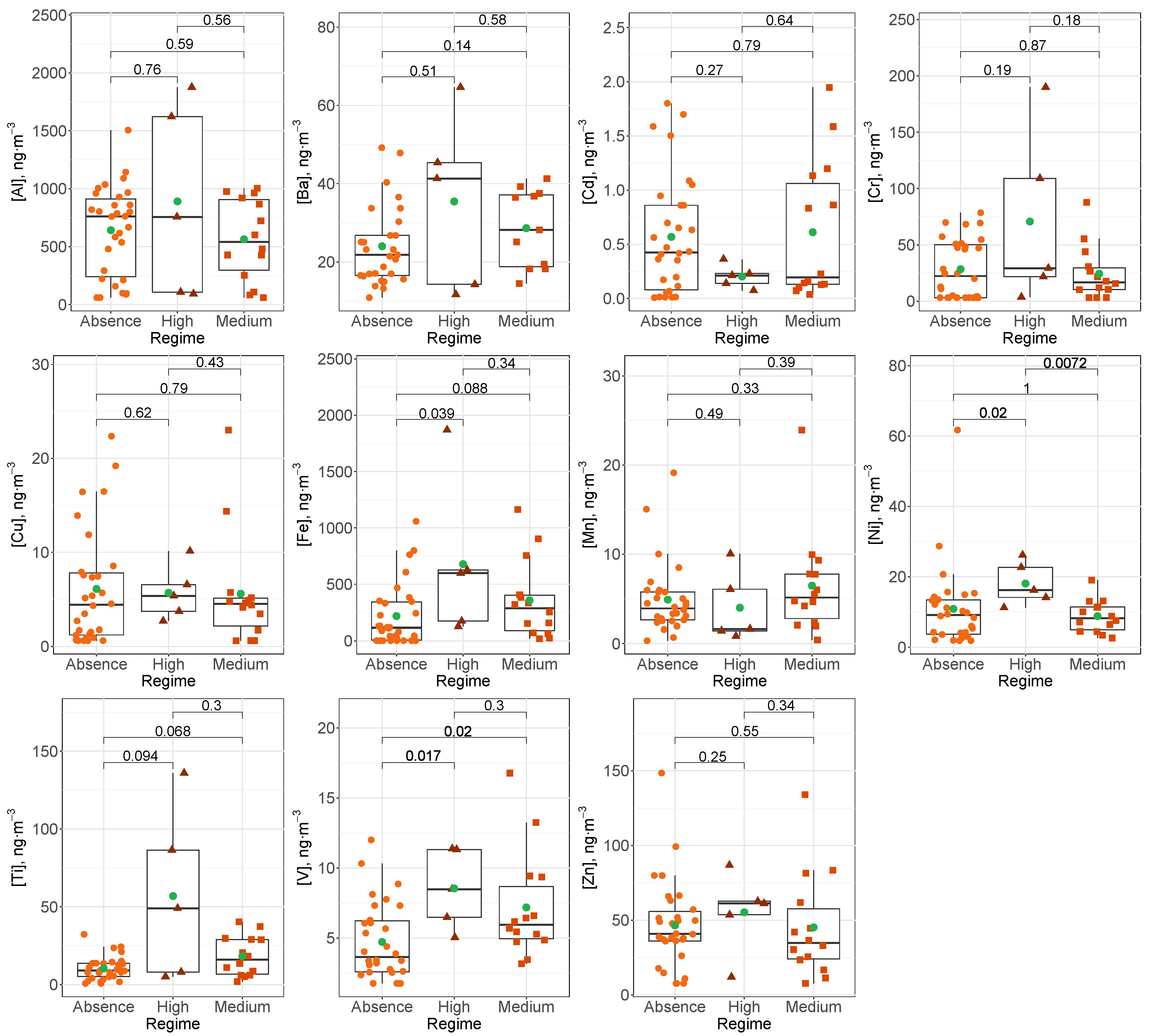
3.1. Descriptive Statistical Analysis
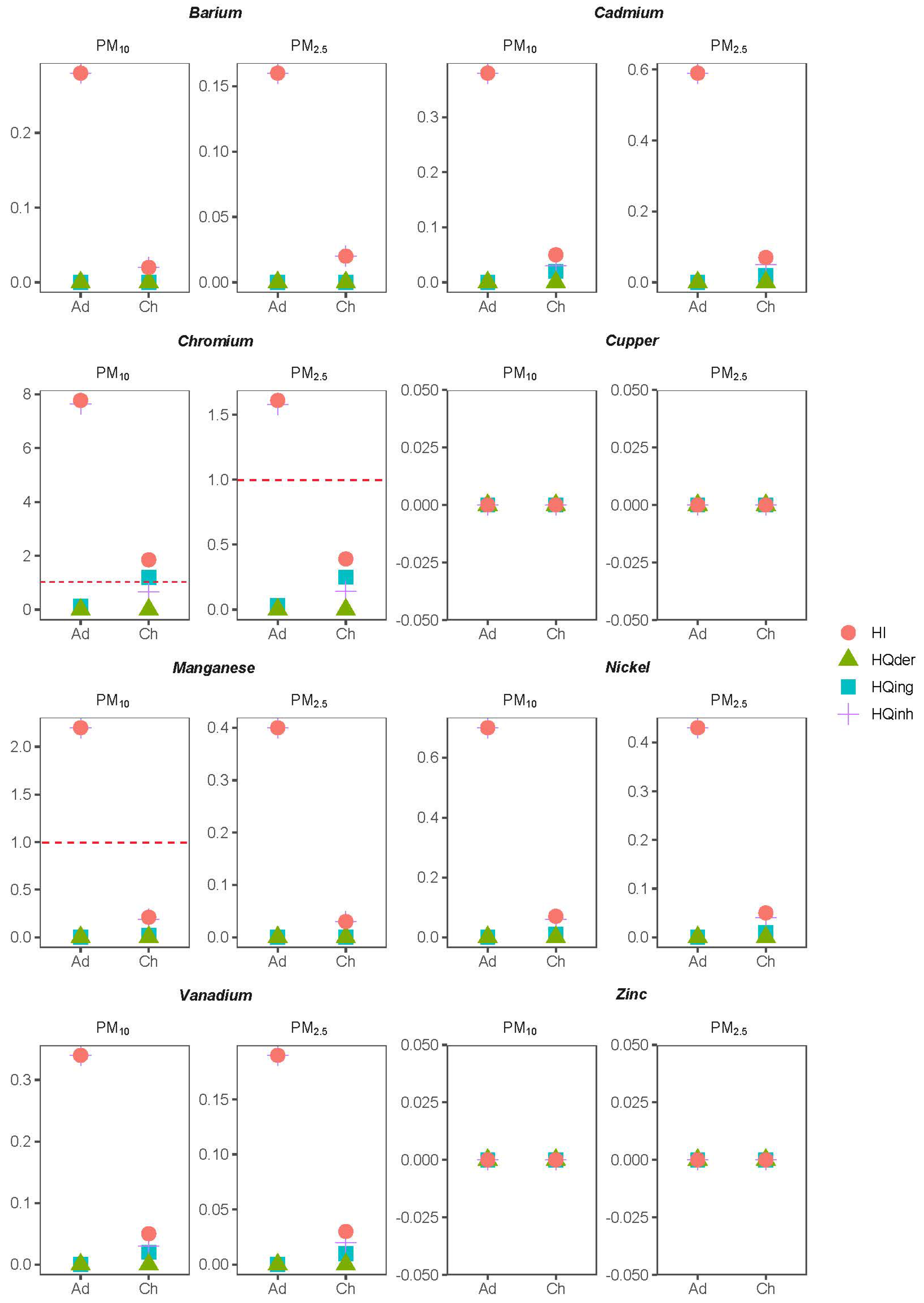
3.2. Health Risk Assessment
3.3. Source Apportionment
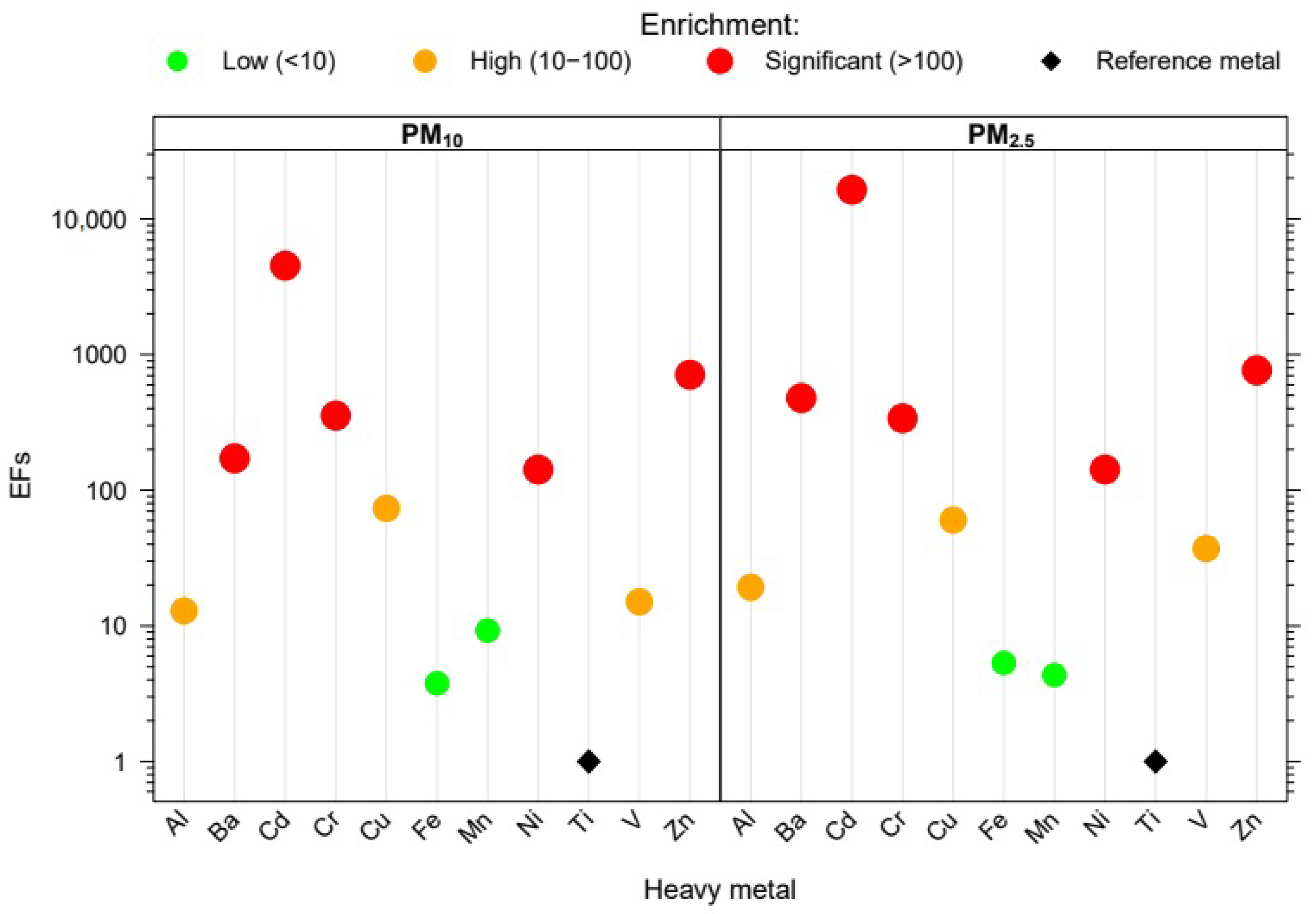
3.3.1. Enrichment Factors
3.3.2. Positive Matrix Factorization
- PM emission sources
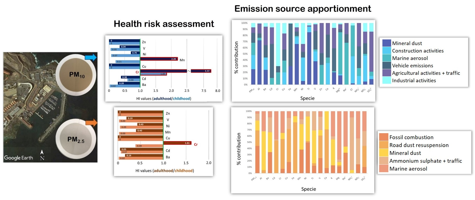
- The percentage contribution of each factor to the concentration of the studied metal species is shown in Table 5. The factors are listed from highest to lowest contribution to the concentration of PM and whose sum is equal to 100.
- The first factor showed high contributions of Al, Ti and Mn (>60%) and, to a lesser extent, contributions of Fe, V, Ba and K (between 20 and 40%), which have a predominantly mineral origin [33]. According to the change in the contribution of this factor, this crustal matter was dominated by the Saharan dust outbreaks, with important contribution values observed during these events. Likewise, high contributions of Cl and NO, possibly due to the presence of halite and sodium nitrate (aged marine aerosol) were observed. These two ions were also explained by the second factor, which may be associated with construction activities carried out during the sampling period. Both Cl and NO are typically used as Portland cement additives to accelerate setting times, among other benefits [34]. The presence of Ba, Cu, Mn and Ni in this factor could be due to exhaust emissions from vehicles used on construction sites, used as diesel additives [35] and emitted as combustion sub-products [31,36]. Finally, Cl was also explained by the third factor, as was the Na and a slight contribution of SO, which suggests that this factor could corresponds to marine aerosol emission [30], due to the sampling site’s proximity to the coast.
- The fourth factor is entirely accounted for by vehicle emissions, with a predominance of non-exhaust emissions. The intense Fe contribution in this factor can be explained by wear on brake pads, since it is their main component [32]. Other elements explained by this factor and associated with these emissions are Ba (used as filler material and considered a tracer [37]), Cu (used in reinforcement fibers [38]) and Al and Cr (employed in abrasives [38]). The second type of non-exhaust emissions corresponds to road dust re-suspension from the circulation of vehicles, with high percentages of Ca [39], K and V. The third type is due to tire wear, which could explain the contribution of this factor to the concentration of Zn, used as a vulcanization agent and the main source of ambient Zn [39]. Exhaust emissions may also be the cause of emission of Cd and Zn due to the combustion of lubricating oil [40,41] and of Mn used as a catalyst (MnO) and petrol additive [42].
- The fifth factor was referred as agricultural activities and traffic, and is the main source of NH emission from the use of fertilizers and manure [43]. These agricultural activities could also be responsible for high contributions of Cd and K. The proximity of the highway accounts for the contributions of metals such as Ba, Cu, Zn and Al.
- The sixth factor explained a significant percentage of Cr and, to a lesser extent, Ni, which would indicate a possible industrial source [15]. Likewise, the mechanical abrasion and sanding works in the port [44] and emissions from the aircraft engines that continuously circulate in the area could also be considered a source of Cr emission.
- PM emission sources
- The percentage contributions for each of the factors obtained in PM are shown in Table 6. As in the case of PM, the total sum of the contributions is equal to 100. The high Ni loading in addition to V and SO in the first factor were indicative of emissions from fossil fuel combustion [45]. The low V/Ni ratio, equal to 0.17, showed an additional source of Ni, such as emissions from motor vehicles, particularly, the diesel-powered ones. This fact was confirmed by the presence of other metals such as Ba, Cu and Mn.
- The second factor may correspond to the road dust re-suspension due to high Fe and Ca presence, while the third factor was attributed to mineral dust, as it revealed high percentages of Al, Mn and Ti, which have a predominantly crustal origin, as already commented in the case of PM.
- The fourth factor was characterized by a high NH loading, more than 80%. As already mentioned for PM, agricultural and livestock activities around of the sampling site were two significant sources of this ion. The NH/SO molar ratio was equal to 1.6, indicating that the total ammonium was neutralized by sulfates, since the molar ratio was 2:1. The slight excess of the latter anions could be due to emissions from vehicle traffic, since the presence of Ba, Ti and K was also observed. Following [46], traffic emissions are considered a major sources of these inorganic ions in urban areas, so that the factor was cataloged as “ammonium sulfate + traffic”.
- Marine aerosol also contributed to the PM concentration, but very slightly, constituting the fifth factor and the one with the lowest percentage. This factor was characterized by high Na, Mg and K loading. It is a marine aerosol polluted by anthropogenic sources such as traffic, as indicated by the high contributions of Cd and Al.
4. Conclusions
Author Contributions
Funding
Institutional Review Board Statement
Informed Consent Statement
Data Availability Statement
Conflicts of Interest
Appendix A. Parameters for Health Risks Assessment
Appendix A.1. Calculation Equations
Appendix A.2. Parameter’s Values

| Acronym | Name | Unit | Value | |||||||
|---|---|---|---|---|---|---|---|---|---|---|
| Common parameters | ||||||||||
| EF | Exposure frequency | day·year | 350 | |||||||
| ET | Exposure time | h·day | 24 | |||||||
| ABS | Dermal absorption factor | - | 0.001 | |||||||
| AT | Averaging lifetime | days | 365 × 70 | |||||||
| (for carcinogens) | ||||||||||
| ATn | Average lifetime | hours | 365 × 70 × 24 | |||||||
| (for carcinogens) | ||||||||||
| CF | Unit conversion factor | Kg·g | 10 × 10 | |||||||
| Parameters dependent on life stage: | Childhood | Adulthood | ||||||||
| IR | Ingestion rate | mg·day | 200 | 100 | ||||||
| ED | Exposure duration | year | 6 | 24 | ||||||
| BW | Body weight | Kg | 17 | 70 | ||||||
| AT | Averaging lifetime | days | ED × 70 | |||||||
| (for non carcinogens) | ||||||||||
| ATn | Average lifetime | hours | ED × 70 × 24 | |||||||
| (for non carcinogens) | ||||||||||
| SA | Skin surface area | cm | 2800 | 5700 | ||||||
| AF | Skin adherence factor | mg·cm | 0.2 | 0.07 | ||||||
| Parameters dependent of heavy metals | Ba | Cd | Cr | Cu | Mn | Ni | V | Zn | ||
| RfD | Oral reference doses | mg·(kg·day) | 0.2 | 0.001 | 0.003 | 0.04 | 0.024 | 0.02 | 0.007 | 0.3 |
| RfC | Inhalation reference concentration | mg·m | 0.0005 | 0.00001 | 0.00001 | 0.04 | 0.00005 | 0.00009 | 0.0001 | 0.3 |
| GIABS | Gastrointestinal absorption factor | - | 0.07 | 0.025 | 0.0025 | 1 | 0.04 | 0.04 | 0.026 | 1 |
| Sf | Oral slope factor | (mg·(kg·day)) | - | 6.3 | 0.5 | - | - | - | - | - |
| IUR | Inhalation unit risk | (g·m) | - | - | 0.084 | - | - | - | - | - |
Appendix B. Calculation Procedure with EPA PMF 5.0
Appendix C. Uncertainties Calculation for PMF
Appendix C.1. Particulate Matter
Appendix C.2. Chemical Species
Appendix D. Additional Results from PMF Analysis
| Specie | Category | S/N | Category | S/N |
|---|---|---|---|---|
| PM | PM | |||
| PM | Strong | 10.06 | Strong | 7.1 |
| Al | Strong | 6.8 | Strong | 5.3 |
| Ba | Strong | 2.8 | Strong | 2.0 |
| Cd | Weak | 0.9 | Weak | 0.5 |
| Cr | Strong | 4.1 | Weak | 1.7 |
| Cu | Weak | 1.5 | Weak | 0.6 |
| Fe | Strong | 4.4 | Strong | 2.3 |
| Mn | Strong | 5.5 | Strong | 2.4 |
| Ni | Strong | 3.2 | Weak | 1.9 |
| Ti | Strong | 4.2 | Weak | 1.9 |
| V | Strong | 6.9 | Strong | 6.9 |
| Zn | Weak | 0.2 | Bad | 0.1 |
| Mg | Strong | 5.7 | — | |
| Na | Strong | 7.9 | Strong | 6.4 |
| Cl | Strong | 8.5 | — | |
| SO | Strong | 8.8 | Strong | 9.0 |
| NO | Strong | 8.8 | Strong | 9.0 |
| NH | Strong | 8.3 | Strong | 8.9 |
| Ca | Strong | 6.6 | Strong | 4.4 |
| K | Strong | 8.0 | Strong | 5.9 |
| Mg | — | Strong | 4.5 | |
References
- Li, L.; Zhang, W.; Xie, L.; Jia, S.; Feng, T.; Yu, H.; Huang, J.; Qian, B. Effects of atmospheric particulate matter pollution on sleep disorders and sleep duration: A cross-sectional study in the UK biobank. Sleep Med. 2020, 74, 152–164. [Google Scholar] [CrossRef] [PubMed]
- Kim, K.E.; Cho, D.; Park, H.J. Air pollution and skin diseases: Adverse effects of airborne particulate matter on various skin diseases. Life Sci. 2016, 152, 126–134. [Google Scholar] [CrossRef] [PubMed]
- Kaufman, Y.J.; Tanré, D.; Boucher, O. A satellite view of aerosols in the climate system. Nature 2002, 419, 215–223. [Google Scholar] [CrossRef] [PubMed]
- Zhang, H.; Hu, J.; Kleeman, M.; Ying, Q. Source apportionment of sulphate and nitrate particulate matter in the Eastern United States and effectiveness of emission control programs. Sci. Total Environ. 2014, 490, 171–181. [Google Scholar] [CrossRef]
- Li, H.; Chen, Y.; Zhou, S.; Wang, F.; Yang, T.; Zhu, Y.; Qingwie, M. Change of dominant phytoplankton groups in the eutrophic coastal sea due to atmospheric deposition. Sci. Total Environ. 2021, 753, 141961. [Google Scholar] [CrossRef]
- Moryani, H.T.; Kong, S.; Du, J.; Bao, J. Health risk assessment of heavy metals accumulated on PM2.5 fractioned road dust from two cities of Pakistan. Int. J. Environ. Res. Public Health 2020, 17, 7124. [Google Scholar] [CrossRef]
- Kastury, F.; Smith, E.; Juhasz, A.L. A critical review of approaches and limitations of inhalation bioavailability and bioaccessibility of metal(loid)s from ambient particulate matter or dust. Sci. Total Environ. 2017, 574, 1054–1074. [Google Scholar] [CrossRef]
- Aminiyan, M.M.; Baalousha, M.; Aminiyan, F.M. Evolution of human health risk based on EPA modeling for adults and children and pollution level of potentially toxic metals in Rafsanhan road dust: A case study in a semi-arid region, Iran. Environ. Sci. Pollut. Res. 2018, 25, 19767–19778. [Google Scholar] [CrossRef]
- Liu, P.; Ren, H.; Xu, H.; Lei, Y.; Shen, Z. Assessment of heavy metals characteristics and health risks associated with PM2.5 en Xi’an, the largest city in northwestern, China. Air Qual. Atmos. Health 2018, 11, 1037–1047. [Google Scholar] [CrossRef]
- Zhang, H.; Zhenxing, M.; Huang, K.; Wang, X.; Cheng, L.; Zeng, L.; Zhou, Y.; Jing, T. Multiple exposure pathways and health risk assessment of heavy metal(loid)s for children living in fourth-tier cities in Hubei Province. Environ. Int. 2019, 129, 517–524. [Google Scholar] [CrossRef]
- Morillas, H.; Maguregui, M.; Paris, C.; Bellot-Gurlet, L.; Colomban, P.; Madariaga, J.M. The role of marine aerosol in the formation on double sulfate/nitrate salts in plasters. Microchem. J. 2015, 123, 148–157. [Google Scholar] [CrossRef]
- Rodriguez, S.; Calzolai, G.; Chiari, M.; Nava, S.; García, M.I.; López-Solano, J.; Marrero, C.; López-Darias, J.; Cuevas, E.; Alonso-Pérez, S.; et al. Rapid changes of dust geochemistry in the Saharan Air Layer linked to sources and meteorology. Atmos. Environ. 2020, 223, 117186. [Google Scholar] [CrossRef]
- Saggu, G.S.; Mittal, S.K. Source apportionment of PM10 by positive matrix factorization model at a source region of biomass burning. J. Environ. Manag. 2020, 266, 110545. [Google Scholar] [CrossRef] [PubMed]
- Manousakas, M.; Diapouli, E.; Papaefthymiou, H.; Migliori, A.; Karydas, A.G.; Padilla-Alvarez, R.; Bogovac, M.; Kaiser, R.B.; Jaksic, M.; Bogdanovic-Radovic, I.; et al. Source apportionment by PMF on elemental concentrations obtained by PIXE analysis of PM10 samples collected at the vicinity of lignite power plants and mines in Megalopolis, Greece. Nucl. Instrum. Methods Phys. Res. Sect. Beam Interact. Mater. Atoms 2015, 349, 114–124. [Google Scholar] [CrossRef]
- Sadeghi, B.; Choi, Y.; Yoon, S.; Flynn, J.; Kotsakis, A.; Lee, S. The characterization of fine particulate matter downwind of Houston: Using integrated factor analysis to identify anthropogenic and natural sources. Environ. Pollut. 2020, 262, 114345. [Google Scholar] [CrossRef] [PubMed]
- Blondet, I.; Schreck, E.; Viers, J.; Casas, S.; Jubany, I.; Bahí, N.; Zouiten, C.; Dufréchou, G.; Freydier, R.; Galy-Lacaux, C.; et al. Atmospheric dust characterization in the mining distric of Cartagena-La Unión, Spain: Air quality and health risks assessment. Sci. Total Environ. 2019, 693, 133496. [Google Scholar] [CrossRef]
- Kumar, A.; Chauchan, A.; Arora, S.; Tripathi, A.; Mohammed, S.; Alghanem, S.; Khan, K.A.; Ghramh, H.A.; Özdemir, A.; Ansari, M.J. Chemical analysis of trace metal contamination in the air of industrial area of Gajraula (U.P.), India. J. King Saud Univ.-Sci. 2020, 32, 1106–1110. [Google Scholar] [CrossRef]
- Tyagi, V.; Gurjar, B.; Joshi, N.; Kumar, P. PM10 and heavy metals in suburban and rural atmospheric environments of Norhthern India. Pract. Period. Hazard. Toxic Radioact. Waste Manag. 2012, 16, 175–182. [Google Scholar] [CrossRef]
- Sun, X.; Wang, H.; Guo, Z.; Lu, P.; Song, F.; Liu, L.; Liu, J.; Rose, N.L.; Wang, F. Positive matrix factorization on source apportionment for typical pollutants in different environmental media: A review. Environ. Sci. Process. Impacts 2020, 22, 239–255. [Google Scholar] [CrossRef] [PubMed]
- MohseniBandpi, A.; Eslami, A.; Ghaderpoori, M.; Shahsavani, A.; Jeihooni, A.K.; Ghaderpoury, A.; Alinejad, A. Health risk assessment of heavy metals on PM2.5 in Tehran air, Iran. Data Brief 2018, 17, 347–355. [Google Scholar] [CrossRef]
- Zhang, X.; Eto, Y.; Aikawa, M. Risk assessment and management of PM2.5-bound heavy metals in the urban area of Kitakyushu, Japan. Sci. Total Environ. 2021, 795, 148748. [Google Scholar] [CrossRef] [PubMed]
- Chen, R.; Jia, B.; Tian, Y.; Feng, Y. Source-specific health risk assessment of PM2.5-bound heavy metals based on high time-resolved measurement in a chinese megacity: Insights into seasonal and diurnal variations. Ecotoxicol. Environ. Saf. 2021, 216, 112167. [Google Scholar] [CrossRef] [PubMed]
- Shelley, R.U.; Morton, P.L.; Langing, W.M. Elemental ratios and enrichment factors in aerosols from the US-GEOTRACES North Atlantic transects. Deep-Sea Res. II 2015, 116, 262–272. [Google Scholar] [CrossRef]
- Buck, C.S.; Aguilar-Islas, A.; Marsay, C.; Kadko, D.; Landing, W.M. Trace element concentrations, elemental ratios and enrichment factors observed in aerosol samples collected during the US GEOTRACES eastern Pacific Ocean transect (GP16). Chem. Geol. 2019, 511, 212–224. [Google Scholar] [CrossRef]
- Heldari-Farsani, M.; Shirmardi, M.; Goudarzi, G.; Alavi, N.; Ahmadi-Ankali, K.; Zallaghi, E.; Naimabadi, A.; Hashemzadeh, B. The evaluation of heavy metals concentration related to PM10 in ambient air of Ahvaz City, Irane. J. Adv. Environ. Health Res. 2014, 1, 120–128. [Google Scholar]
- Jochum, K.P.; Nohl, U.; Herwing, K.; Lammel, E.; Stoll, B.; Hofmann, A.W. GeOReM: A new geochemical database for reference materials and isotopic standards. Geostand. Geonalytical Res. 2007, 29, 333–338. [Google Scholar] [CrossRef]
- Hopke, P.K. Review of receptor modeling methods for source apportionment. J. Air Waste Manag. Assoc. 2016, 66, 237–259. [Google Scholar] [CrossRef]
- Mircea, M.; Calori, G.; Pirovano, G.; Bellis, C. European guide on air pollution source apportionment for particulate matter with source oriented models and their combined use with receptor models. EUR 30082 EN Publ. Off. Eur. Union Luxemb. 2008, 10, 142–149. [Google Scholar]
- Bellis, C.A.; Larsen, B.R.; Amato, F.; El Haddad, I.; Favez, O.; Harrison, R.M.; Hopke, P.K.; Nava, S.; Paatero, P.; Prévôt, A.; et al. European Guide on Air Pollution Source Apportionment with Receptor Models; European Commission, EUR 26080 EN; Publications Office of the European Union: Luxembourg, 2013. [Google Scholar]
- Millan-Martinez, M.; Sánchez-Rodas, D.; Sánchez de la Campa, A.; de la Rosa, J. Contribution of anthropogenic and natural sources in PM10 during North African dust events in Southern Europe. Environ. Pollut. 2021, 290, 118065. [Google Scholar] [CrossRef]
- Wang, J.M.; Jeong, C.H.; Healy, R.M.; Sofowote, U.; Debosz, J.; Su, Y.; Munoz, A.; Evans, G.J. Quantifying metal emission from vehicle traffic using real world emissions factors. Environ. Pollut. 2021, 268, 115805. [Google Scholar] [CrossRef]
- Cai, R.; Zhang, J.; Nie, X.; Tjong, J.; Matthews, D.T.A. Wear mechanism evolution on brake discs for reduced wear and particulate emissions. Wear 2020, 452–453, 203283. [Google Scholar] [CrossRef]
- Lokorai, K.; Ali-Khodja, H.; Khardi, S.; Bencharif-Madani, F.; Naidja, L.; Bouziane, M. Influence of mineral dust on the concentration and composition of PM10 in the city of Constantine. Aeolian Res. 2021, 50, 100677. [Google Scholar] [CrossRef]
- Dorn, T.; Blask, O.; Stephan, D. Acceleration of cement hydration—A review of the working mechanisms, effects on setting time, and compressive strength development of accelerating admixtures. Contruction Build. Mater. 2022, 323, 126554. [Google Scholar] [CrossRef]
- Hosseinzadeh-Bandbafha, H.; Tabatebaei, M.; Aghbashlo, M.; Khanali, M.; Demirbas, A. A comprehensive review on the environmental impacts of diesel/biodiesel additives. Energy Convers. Manag. 2018, 174, 579–614. [Google Scholar] [CrossRef]
- Tian, H.Z.; Lu, L.; Cheng, K.; Hao, J.M.; Zhao, D.; Wang, Y.; Jia, W.X.; Qiu, P.P. Anthropogenic atmospheric nickel emissions and its distribution characteristics in China. Sci. Total Environ. 2012, 417–418, 148–157. [Google Scholar] [CrossRef]
- Beddows, D.C.S.; Dall’Osto, M.; Olatunbosum, O.A.; Harrison, R.M. Detection of brake wear aerosols by aerosol time-of-flight mass spectrometry. Atmos. Environ. 2016, 129, 167–175. [Google Scholar] [CrossRef]
- Thorpe, A.; Harrison, R.M. Sources and properties of non-exhaust particulate matter from road traffic: A review. Sci. Total Environ. 2008, 400, 270–282. [Google Scholar] [CrossRef]
- Amato, F.; Alastuey, A.; Karanasiou, A.; Lucarelli, F.; Nava, S.; Calzolai, G.; Severi, M.; Becagli, M.; Gianelle, V.L.; Colombi, C.; et al. AIRUSE-LIFE+: A harmonized PM speciation and source apportionment in five southern European cities. Atmos. Chem. Phys. 2016, 16, 3289–3309. [Google Scholar] [CrossRef]
- Hao, Y.; Meng, X.; Yu, X.; Lei, M.; Li, W.; Shi, F.; Yang, W.; Zhang, S.; Xie, S. Characteristics of trace elements in PM2.5 and PM10 of Chifeng, northeast China: Insights into spatiotemporal variations and sources. Atmos. Res. 2018, 213, 550–561. [Google Scholar] [CrossRef]
- Li, W.; Dryfhout-Clark, H.; Hung, H. PM10-bound trace elements in the Great Lakes Basin (1988–2017) indicates effectiveness of regulatory actions, variations in sources and reduction in human health risks. Environ. Int. 2020, 143, 106008. [Google Scholar] [CrossRef]
- Ghosh, S.; Rabba, R.; Chowdhury, M.; Padhy, P.K. Source and chemical species characterization of PM10 and human health risk assessment of semi-urban, urban and industrial areas of West Bengal, India. Chemosphere 2018, 207, 626–636. [Google Scholar] [CrossRef] [PubMed]
- Kabelitz, T.; Ammon, C.; Funk, R.; Münch, S.; Biniasch, O.; Nübel, U.; Thiel, N.; Rösler, U.; Siller, P.; Amon, B.; et al. Functional relationship of particulate matter (PM) emissions, animal species, and moisture content during manure application. Environ. Int. 2020, 143, 105577. [Google Scholar] [CrossRef] [PubMed]
- Wu, S.H.; Cai, M.J.; Xu, C.; Zhang, N.; Zhou, J.B.; Yan, J.P.; Schwab, J.J.; Yuan, C.S. Chemical nature of PM2.5 and PM10 in the coastal urban Xiamen, China: Insights into the impacts of shipping emissions and health risk. Atmos. Environ. 2020, 227, 117383. [Google Scholar] [CrossRef]
- Moreno, T.; Querol, X.; Alastuey, A.; de la Rosa, J.; Sánchez de la Campa, A.M.; Minguillón, M.; Pandolfi, M.; González-Castanedo, Y.; Monfort, E.; Gibbons, W. Variations in Vanadium, nickel and lanthnoid element concentrations in urban air. Sci. Total Environ. 2010, 408, 4569–4579. [Google Scholar] [CrossRef] [PubMed]
- Xing, W.; Yang, L.; Zhang, H.; Zhang, X.; Wang, Y.; Bai, P.; Zhang, L.; Hayakawa, K.; Nagao, S.; Tang, N. Variations in traffic-related water soluble inorganic ions in PM2.5 in Kanazawa, Japan, after the implementation of a new vehicle emissions regulation. Atmos. Pollut. Res. 2021, 12, 101233. [Google Scholar] [CrossRef]
- Paatero, P.; Hopke, P.K. Discarding or downweighting high-noise variables in factor analytic models. Anal. Chim. Acta 2003, 490, 277–289. [Google Scholar] [CrossRef]
- Paatero, P.; Hopke, P.K. Rotational tools for factor analytic models. Chemometrics 2009, 23, 91–100. [Google Scholar] [CrossRef]
- Alvi, M.U.; Kistler, M.; Mahmud, T.; Shahid, I.; Alam, K.; Chisthie, F.; Hussain, R.; Kasper-Giebl, A. The composition and sources of water soluble ions in PM10 at an urban site in the Indo-Ganfetic Plain. J. Atmos. Sol.-Terr. Phys. 2019, 196, 105142. [Google Scholar] [CrossRef]
- Paatero, P.; Hopke, P.K.; Begum, B.A.; Biswas, S.K. A graphical diagnostic method for assessing the rotation in factor analytical models of atmospheric pollution. Atmos. Environ. 2005, 39, 193–201. [Google Scholar] [CrossRef]
- Zabalza, J.; Ogulei, D.; Hopke, P.; Lee, J.; Hwang, I.; Querol, X.; Alastuey, A.; Santamaria, J. Concentration and sources of PM10 and its constituents in Alsasua, Spain. Water Air Soil Pollut. 2006, 174, 385–404. [Google Scholar] [CrossRef]


| Type of Risk | Value | Risk Level |
|---|---|---|
| Chronic (non-carcinogenic) | HI ≥ 1 | Causal effects |
| HI < 1 | Non causal effects | |
| Carcinogenic | TCR ≥ 10 | Very high |
| 10 ≤ TCR <10 | High | |
| 10 ≤ TCR < 10 | Moderate | |
| 10 ≤ TCR < 10 | Low | |
| TCR < 10 | Very low |
| Metal | Size | ± | CV | Max | Min |
|---|---|---|---|---|---|
| Al | PM | 2430.93 ± 3306.55 | 136 | 15,897.77 | 13.00 |
| PM | 645.00 ± 435.69 | 68 | 875.99 | 59.78 | |
| Ba | PM | 38.40 ± 20.35 | 53 | 115.25 | 12.00 |
| PM | 26.39 ± 12.09 | 46 | 64.63 | 10.86 | |
| Cd | PM | 0.91 ± 0.71 | 78 | 2.74 | 0.02 |
| PM | 0.54 ± 0.55 | 102 | 1.95 | 0.01 | |
| Cr | PM | 114.41 ± 136.81 | 120 | 856.66 | 0.58 |
| PM | 31.59 ± 35.36 | 112 | 189.88 | 3.19 | |
| Cu | PM | 12.01 ± 9.31 | 78 | 49.34 | 0.34 |
| PM | 5.91 ± 5.79 | 98 | 23.02 | 0.62 | |
| Fe | PM | 1062.48 ± 1617.88 | 152 | 8169.59 | 2.73 |
| PM | 304.44 ± 375.77 | 123 | 1869.68 | 1.58 | |
| Mn | PM | 27.73 ± 31.79 | 115 | 166.76 | 1.05 |
| PM | 5.26 ± 4.54 | 86 | 23.93 | 0.33 | |
| Ni | PM | 18.81 ± 10.80 | 57 | 63.53 | 2.35 |
| PM | 10.96 ± 9.78 | 89 | 61.72 | 1.87 | |
| Ti | PM | 89.85 ± 131.19 | 146 | 630.16 | 2.66 |
| PM | 17.41 ± 22.95 | 132 | 135.96 | 0.76 | |
| V | PM | 9.90 ± 8.28 | 84 | 38.45 | 2.16 |
| PM | 5.81 ± 3.37 | 58 | 16.78 | 1.76 | |
| Zn | PM | 74.81 ± 70.39 | 94 | 391.32 | 10.90 |
| PM | 46.98 ± 30.38 | 65 | 148.41 | 7.65 |
| Heavy Metal | Childhood | Adulthood |
|---|---|---|
| Cd | 9.04 × 10 | 3.62 × 10 |
| Cr | 5.33 × 10 | 2.13 × 10 |
| Ni | 9.97 × 10 | 3.99 × 10 |
| Heavy Metal | Childhood | Adulthood |
|---|---|---|
| Cd | 5.83 × 10 | 2.33 × 10 |
| Cr | 1.14 × 10 | 4.54 × 10 |
| Ni | 1.61 × 10 | 6.44 × 10 |
| Species | Factor 1 | Factor 2 | Factor 3 | Factor 4 | Factor 5 | Factor 6 |
|---|---|---|---|---|---|---|
| PM | 25 | 23 | 19 | 16 | 9 | 7 |
| Al | 72 | 0 | 4 | 7 | 16 | 1 |
| Ba | 24 | 20 | 0 | 20 | 30 | 6 |
| Cd | 0 | 0 | 11 | 54 | 27 | 7 |
| Cr | 0 | 0 | 20 | 10 | 0 | 70 |
| Cu | 0 | 21 | 19 | 18 | 26 | 17 |
| Fe | 30 | 0 | 0 | 69 | 0 | 1 |
| Mn | 65 | 11 | 2 | 7 | 7 | 7 |
| Ni | 6 | 37 | 0 | 9 | 13 | 34 |
| Ti | 85 | 9 | 0 | 0 | 2 | 4 |
| V | 37 | 16 | 3 | 30 | 11 | 2 |
| Zn | 0 | 0 | 32 | 19 | 49 | 0 |
| Ca | 0 | 35 | 9 | 37 | 19 | 0 |
| K | 20 | 0 | 2 | 37 | 33 | 8 |
| Mg | 15 | 2 | 68 | 5 | 8 | 2 |
| Na | 0 | 0 | 69 | 14 | 18 | 0 |
| Cl | 2 | 44 | 51 | 0 | 0 | 4 |
| NH | 9 | 5 | 7 | 0 | 64 | 14 |
| NO | 5 | 42 | 3 | 17 | 19 | 14 |
| SO | 0 | 14 | 13 | 35 | 39 | 0 |
| Species | Factor 1 | Factor 2 | Factor 3 | Factor 4 | Factor 5 |
|---|---|---|---|---|---|
| PM | 44 | 25 | 16 | 11 | 4 |
| Al | 0 | 5 | 63 | 1 | 32 |
| Ba | 34 | 0 | 32 | 24 | 10 |
| Cd | 0 | 52 | 0 | 2 | 45 |
| Cr | 7 | 48 | 10 | 0 | 35 |
| Cu | 18 | 53 | 0 | 18 | 11 |
| Fe | 0 | 82 | 10 | 0 | 8 |
| Mn | 38 | 0 | 41 | 8 | 13 |
| Ni | 70 | 2 | 32 | 7 | 0 |
| Ti | 12 | 4 | 53 | 31 | 0 |
| V | 24 | 36 | 9 | 21 | 9 |
| Ca | 9 | 68 | 32 | 0 | 0 |
| K | 10 | 0 | 33 | 4 | 52 |
| Mg | 11 | 2 | 5 | 4 | 78 |
| Na | 33 | 0 | 10 | 0 | 57 |
| NH | 0 | 0 | 5 | 85 | 10 |
| NO | 14 | 0 | 0 | 41 | 43 |
| SO | 10 | 34 | 0 | 24 | 32 |
Disclaimer/Publisher’s Note: The statements, opinions and data contained in all publications are solely those of the individual author(s) and contributor(s) and not of MDPI and/or the editor(s). MDPI and/or the editor(s) disclaim responsibility for any injury to people or property resulting from any ideas, methods, instructions or products referred to in the content. |
© 2023 by the authors. Licensee MDPI, Basel, Switzerland. This article is an open access article distributed under the terms and conditions of the Creative Commons Attribution (CC BY) license (https://creativecommons.org/licenses/by/4.0/).
Share and Cite
Martín-Cruz, Y.; Gómez-Losada, Á. Risk Assessment and Source Apportionment of Metals on Atmospheric Particulate Matter in a Suburban Background Area of Gran Canaria (Spain). Int. J. Environ. Res. Public Health 2023, 20, 5763. https://0-doi-org.brum.beds.ac.uk/10.3390/ijerph20105763
Martín-Cruz Y, Gómez-Losada Á. Risk Assessment and Source Apportionment of Metals on Atmospheric Particulate Matter in a Suburban Background Area of Gran Canaria (Spain). International Journal of Environmental Research and Public Health. 2023; 20(10):5763. https://0-doi-org.brum.beds.ac.uk/10.3390/ijerph20105763
Chicago/Turabian StyleMartín-Cruz, Yumara, and Álvaro Gómez-Losada. 2023. "Risk Assessment and Source Apportionment of Metals on Atmospheric Particulate Matter in a Suburban Background Area of Gran Canaria (Spain)" International Journal of Environmental Research and Public Health 20, no. 10: 5763. https://0-doi-org.brum.beds.ac.uk/10.3390/ijerph20105763