Multiscale Decomposition and Spectral Analysis of Sector ETF Price Dynamics

Abstract

We present a multiscale analysis of the price dynamics of U.S. sector exchange-traded funds (ETFs). Our methodology features a multiscale noise-assisted approach, called the complementary ensemble empirical mode decomposition (CEEMD), that decomposes any financial time series into a number of intrinsic mode functions from high to low frequencies. By combining high-frequency modes or low-frequency modes, we show how to filter the financial time series and estimate conditional volatilities. The results show the different dynamics of the sector ETFs on multiple timescales. We then apply Hilbert spectral analysis to derive the instantaneous energy-frequency spectrum of each sector ETF. Using historical ETF prices, we illustrate and compare the properties of various timescales embedded in the original time series. Through the new metrics of the Hilbert power spectrum and frequency deviation, we are able to identify differences among sector ETF and with respect to SPY that were not obvious before.

1. Introduction

Asset prices are driven by factors of different timescales, ranging from long-term market regimes to short-term fluctuations. Many market observations and empirical studies (Fouque et al. 2003; In and Kim 2012; Maghyereh et al. 2019; Yahya et al. 2019) suggest that many financial time series often exhibit nonstationary behaviors, such as time-varying volatility and trends. These characteristics can hardly be captured by linear models and call for an adaptive and nonlinear approach for analysis.

One approach for analyzing nonstationary time series is the Hilbert-Huang transform (HHT) introduced by Huang et al. (1998). The HHT method can decompose any time series into oscillating components with nonstationary amplitudes and frequencies using empirical mode decomposition (EMD). This fully adaptive method provides a multiscale decomposition for the original time series, which gives richer information about the time series. The instantaneous frequency and instantaneous amplitude of each component are later extracted using the Hilbert transform. The decomposition onto different timescales also allows for reconstruction up to different resolutions, providing a smoothing and filtering tool that is ideal for noisy financial time series.

As discussed in Huang (2014), the method of HHT and its variations have been applied in numerous fields, from engineering to geophysics. Applications of HHT to finance date back to the work by Huang and co-authors on modeling mortgage rate data (Huang et al. 2003). Empirical mode decomposition (EMD) has been used for financial time series forecasting (Nava et al. 2018b; Wang and Wang 2017) and for examining the correlation between financial time series (Nava et al. 2018a).

In terms of methodology, there have been several studies on the variations and alternatives to EMD, including optimization-based methods (Hou and Shi 2011, 2013; Hou et al. 2009; Huang and Kunoth 2013), ensemble empirical-mode decomposition (EEMD) for tackling mode mixing (Wu and Huang 2009), and noise-assisted alternative approaches (Yeh et al. 2010).

For financial time series with high levels of intrinsic noise, we apply the complementary ensemble empirical mode decomposition (CEEMD). Like EMD, CEEMD decomposes any time series—stationary or not—into a number of intrinsic mode functions representing the local characteristics of the time series at different timescales, but the timescale separation is improved by resolving mode mixing in EMD (Huang et al. 1999). The noise-assisted approach is also more robust to intrinsic noise in the data. CEEMD have been found to be useful for forecasting (Niu et al. 2016; Tang et al. 2015) and signal processing Li et al. (2015). In our companion papers Leung and Zhao (2021a, 2021b), we introduce variations of the complementary ensemble EMD method to analyze cryptocurrency and equity prices, respectively.

We focus our study on the multiscale analysis of sector ETF price dynamics. Our noise-assisted approach decomposes any financial time series into a number of intrinsic mode functions, along with the corresponding instantaneous amplitudes and instantaneous frequencies. Different combinations of modes allow us to reconstruct the time series using components of different timescales. We then apply Hilbert spectral analysis to define and compute the associated instantaneous energy-frequency spectrum to illustrate the properties of various timescales embedded in the original time series. In particular, we derive and compute the central frequency associated with a collection of sector ETFs, which allows us to compare the distinct behaviors of ETF prices.

In the literature, there are relatively few studies that examine and compare the price dynamics of sector ETFs. In Arugaslan and Samant (2014), traditional statistical estimation techniques are used to compare the price dynamics of ETFs. In Tiwari et al. (2017), the authors use multifractal detrended fluctuation analysis (MF-DFA) and the Hurst exponent to show that the sector ETF market is multifractal. They also argue that the dynamics on long and short timescales challenge the market efficiency hypothesis. Similar studies in other markets can also be found in Aloui et al. (2018); Mensi et al. (2017); Yang et al. (2016). These studies provide evidence and motivation that multiscale analysis is necessary to fully understand the price dynamics of various assets.

Our primary objective is to present a new method to analyze sector ETFs on a multiscale level. Comparing to previous studies, our methodology provides a new multiscale time-frequency perspective to investigate sector ETF price dynamics. To our best knowledge, our study is the first application of CEEMD to sector ETFs, and our Hilbert spectral analysis and derivation of power spectrum for sector ETFs are also new.

Moreover, our approach is a fully data-driven method and flexible to adapt to the different timescales embedded in the time series. Through the new metrics like filtered conditional volatility and the Hilbert power spectrum, we provide new ways to discern differences among sector ETFs that are hidden in certain timescales. For example, we introduce frequency deviation in order to measure the synchronization between a sector ETF and the market index.

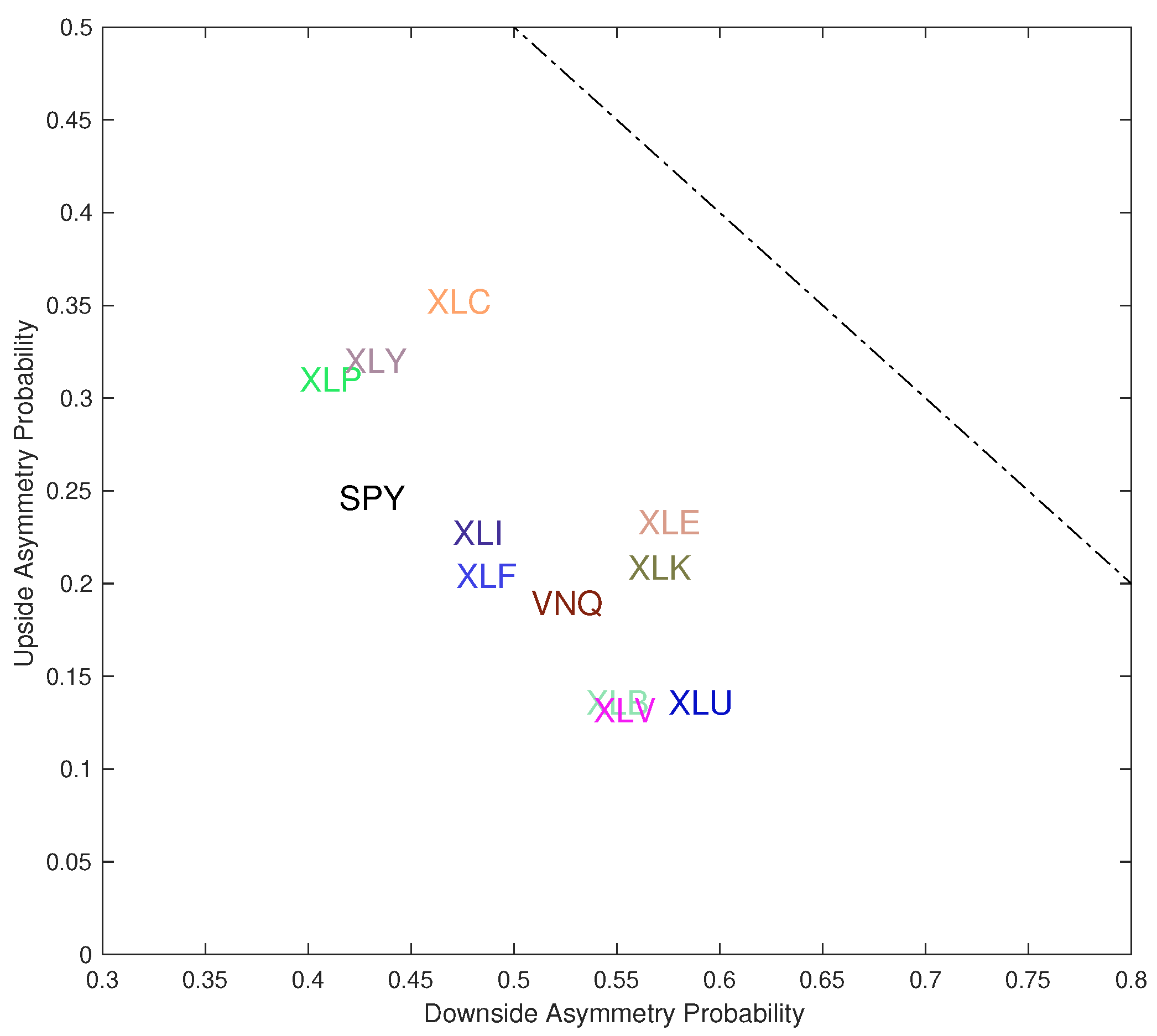
Among our results, we find that sector ETFs exhibit different degrees of volatility asymmetry. Perhaps surprisingly, some sector ETFs, such as XLP, XLY, and XLC, tend to have higher volatility in an upside market than that in a downside market.

The rest of the paper is structured as follows. We present our time series decomposition method in Section 2. As a direct application, CEEMD is used for filtering ETF time series in Section 3. In Section 4, we discuss the estimation of multiscale conditional volatilities and compare them across sector ETFs. In Section 5, we derive the energy-frequency spectra of various sector ETFs and provide a comparative analysis. Lastly, concluding remarks are provided in Section 6.

2. Multiscale Decomposition Methodology

For our analysis of financial time series, a major building block is the empirical mode decomposition (EMD) introduced by Huang et al. (1998). In its simplest form, this method iteratively decomposes a time series $x(t)$ into a finite sequence of oscillating components $c_1(t),\cdots ,c_n(t)$, plus a nonoscillatory trend called the residual term $r_n(t)$. Precisely, we have

$$x(t)=\sum _{j=1}^n{c}_j(t)+r_n(t).$$

(1)

The resulting components $c_j(t)$s are called intrinsic mode functions (IMFs) by Huang et al. (1998). They have certain oscillatory properties and admit well-behaved and physically meaningful Hilbert transform. For each IMF, the numbers of extrema and zero crossings must be equal or at most, differ by one, and the maxima of the function defined by the upper envelope and the minima defined by the lower envelope must sum up to zero at any time. These conditions ensure pure oscillation while allowing time-varying frequency and amplitude. Mathematically, an IMF $c(t)$ can be expressed as

$$c(t)=a(t)cos(\theta (t)),$$

(2)

where $a(t)\ge 0$ is the instantaneous amplitude, and $\theta (t)$ is the phase function with ${\theta }^{\prime }(t)\ge 0$.

2.1. EMD Algorithm and Variations

In other words, the standard EMD algorithm (Huang et al. 1998; Rilling et al. 2003) is a sifting process that decomposes any time series into a finite set of IMFs that oscillate on different timescales, plus a nonoscillatory residual term. The key idea is as follows: look for the finest oscillation by finding all the local maxima and minima, and then subtract the remaining trend until the oscillation satisfies the IMF conditions. Each IMF discovered is removed sequentially from the time series until a nonoscillatory residual term remains. The residual term is a constant or monotonic function, or has, at most, one maximum or minimum.

The algorithm is summarized as follows:

• Initialize the residual term as $r_0(t)=x(t)$ and set $j=1$.
• While $r_{j-1}(t)$ is not nonoscillatory, which means having more than one maximum/ minimum, apply the following sifting process:
• Initialize the component as $c_j(t)=r_{j-1}(t)$.

  –

  Interpolate the maxima of $c_j(t)$ using a cubic spline as the upper envelope $u(t)$, and interpolate the minima of $c_j(t)$ using a cubic spline as the lower envelope $l(t)$. Compute the mean of the upper and lower envelopes $m(t)=\frac{1}{2}\left(u(t)+l(t)\right)$.

  –

  Iterate $c_j(t)\leftarrow c_j(t)-m(t)$.

  –

  Stop when $c_j(t)$ satisfies the criteria of an IMF. Let $c_j(t)$ be the j-th component, and iterate $r_j(t)=r_{j-1}(t)-c_j(t)$ and $j\leftarrow j+1$.

• Return the IMFs $c_1(t),\cdots ,c_n(t)$, and the residual term $r_n(t)$.

This algorithm is purely empirically driven and adaptive with minimal assumption on temporal changes and distributional properties, making it ideal for nonstationary financial time series.

When decomposing a time series into IMF components of different frequencies, the phenomenon of mode mixing may arise. Mode mixing is defined as either one IMF consisting of widely disparate scales, or signals of similar scales residing in several IMF components (Huang et al. 1999; Wu and Huang 2009). This problem poses potential challenges on the interpretation of IMFs, and can be exacerbated by the high degrees of nonstationarity and noise commonly observed in sector ETF prices.

The ensemble empirical mode decomposition (EEMD) was proposed by Wu and Huang (2009) to resolve the mode mixing issue. It is a noise-assisted signal processing technique that extracts each component from an ensemble mean computed based on N trials. In each trial i, an i.i.d. white noise $w_i(t)$ with a zero mean and finite variance is added to the original time series $x(t)$, and $x(t)+w_i(t)$ is referred to as the signal in this trial. The plain EMD algorithm is then applied to the signal, outputting the IMFs $c_{ij}(t),j=1,\cdots ,n$, and the residual term $r_{in}(t)$. Finally, the ensemble mean of the IMF components and residual terms across all the N trails is regarded as the true mode extraction. The components are given by

$$c_j(t)=\frac{1}{N}\sum _{i=1}^N{c}_{ij}(t),r_n=\frac{1}{N}\sum _{i=1}^N{r}_{in}(t).$$

(3)

Applying these to (1), we obtain

$$\sum _{j=1}^n{c}_{ij}(t)+r_{in}(t)=x(t)+w_i(t).$$

(4)

Summing up (4) over the trials divided by N, the ensemble mean of the IMF components is $x(t)+\frac{1}{N}{\sum }_{i=1}^N{w}_i(t)$, which converges to the original time series $x(t)$ almost surely at the rate of $\mathcal{O}(\frac{1}{\sqrt{N}})$.

Hence, a large ensemble size is desired, though it can also be prohibitive in terms of computational cost and speed. To address this particular issue, Yeh et al. (2010) introduced the complementary ensemble EMD (CEEMD) method. CEEMD adds a complementary negative noise $-w_i(t)$ to the ensemble for each trial, thus expanding the total ensemble size to $2N$. The components from the ensemble mean sum up to equal the original time series:

$$\sum _{j=1}^n{c}_j(t)+r_n(t)=x(t)+\frac{1}{2N}\sum _{i=1}^N(w_i(t)-w_i(t))=x(t).$$

(5)

This holds exactly regardless of the choice of N, thus reducing the need to have a very large ensemble size. In addition to reducing mode mixing, CEEMD is also more robust to intrinsic noise in the original data, as it automatically averages out extra independent noises in the process.

2.2. CEEMD for Sector ETFs

We now apply CEEMD to analyze the empirical price dynamics of U.S. sector ETFs. As summarized in

Table 1. List of U.S. sector ETFs ranked by asset under management (AUM). Source: ETF fact sheets by Vanguard and State Street Global Advisors as of 30 June 2021.

Sector	ETF Ticker	# Holdings	AUM ($b)
Real Estate	VNQ	174	77.50
Technology	XLK	74	44.19
Financials	XLF	65	39.30
Health Care	XLV	64	31.19
Energy	XLE	22	22.58
Consumer Discretionary	XLY	63	19.72
Industrials	XLI	74	19.40
Communication Services	XLC	26	13.93
Consumer Staples	XLP	32	12.36
Utilities	XLU	28	11.78
Materials	XLB	28	8.59

, there are, in total, eleven funds representing all the sectors in the U.S. market. Each ETF represents a portfolio of equities within the corresponding sector. The ETFs hold different numbers of stocks, and their assets under management (AUM) range from under U.S.$10 bil to over U.S.$70 bil. All these sector ETFs, except the real estate sector ETF VNQ, are the Select Sector SPDR Funds issued by State Street Global Advisors (SSGA). SSGA also has a real estate sector ETF (ticker: XLRE), but its AUM is much smaller than a similar fund, VNQ, issued by Vanguard. Hence, we select VNQ over XLRE as the real estate sector ETF in our study. Moreover, the communication services sector ETF XLC has the shortest price history since it was created in June 2018. To make a fair comparison across all the ETFs, we fix the common time frame from 20 June 2018 to 15 June 2021 to accommodate for the shortest price history of the ETFs in Table 1.

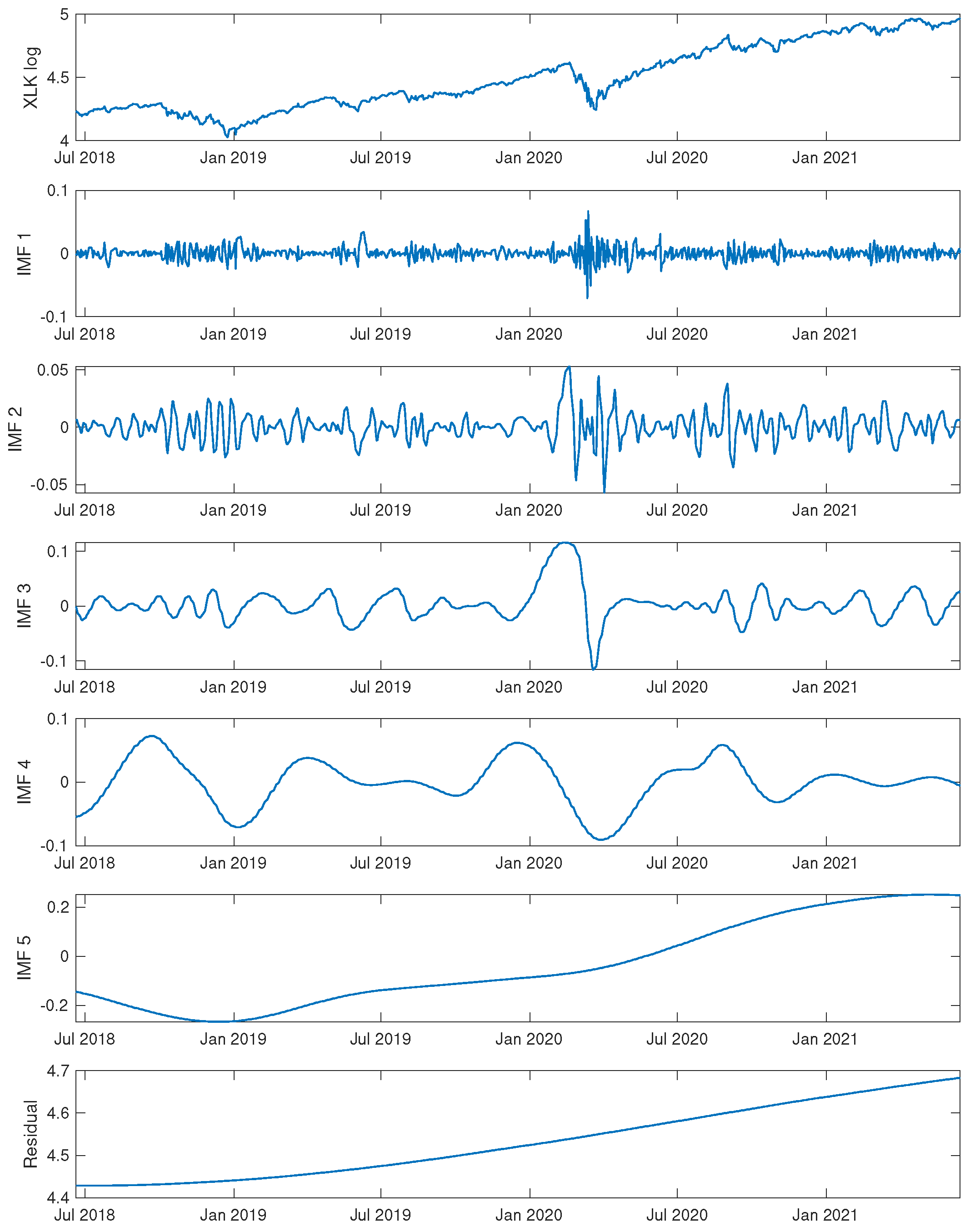
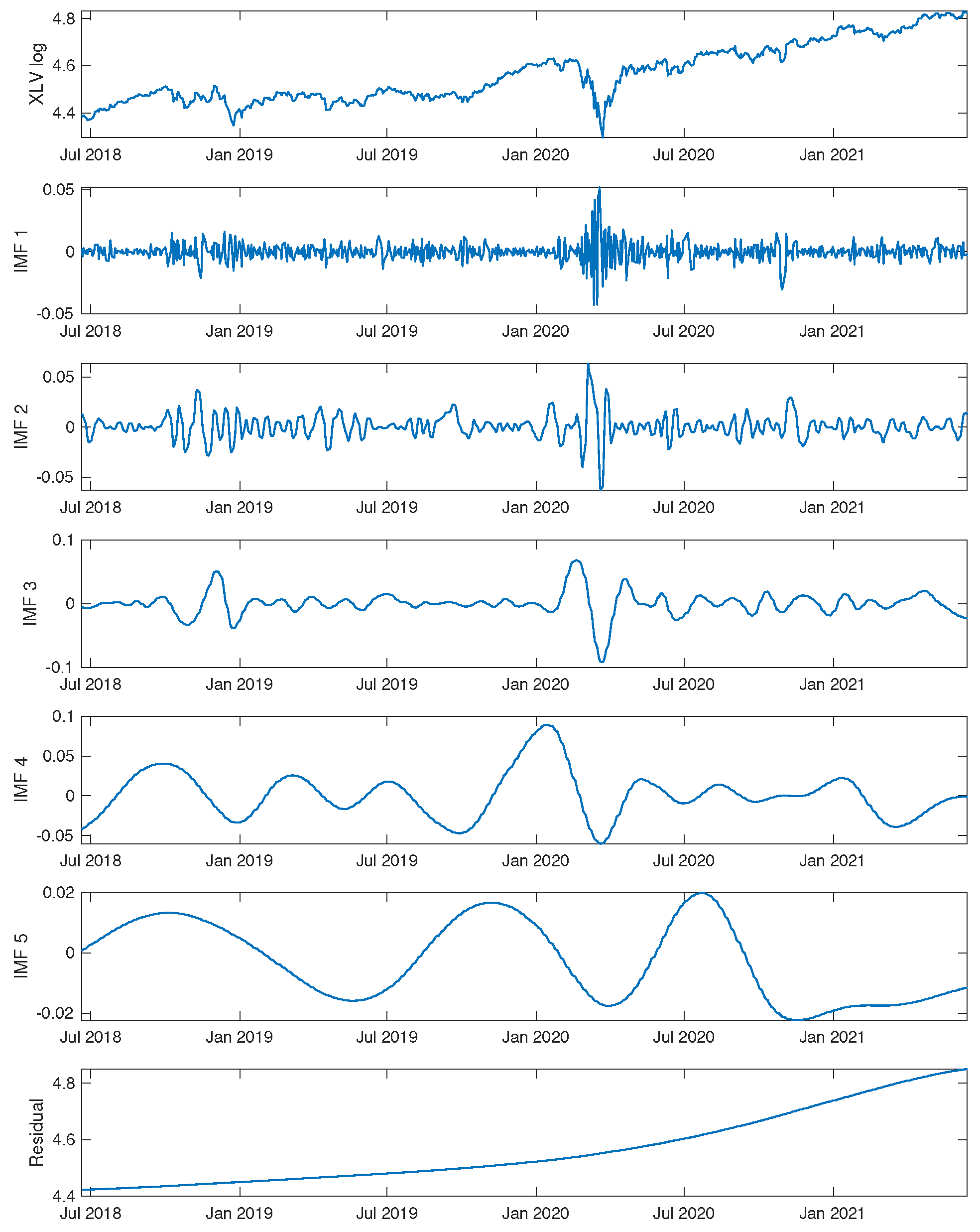
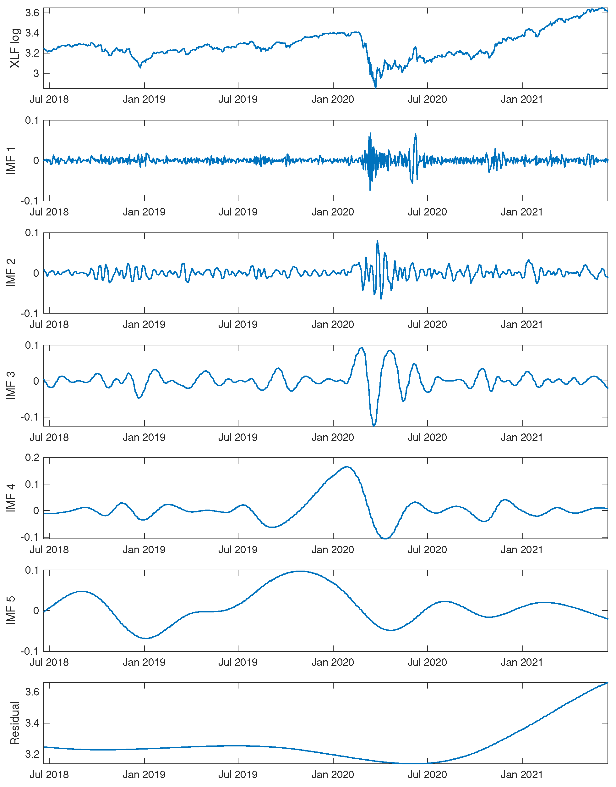
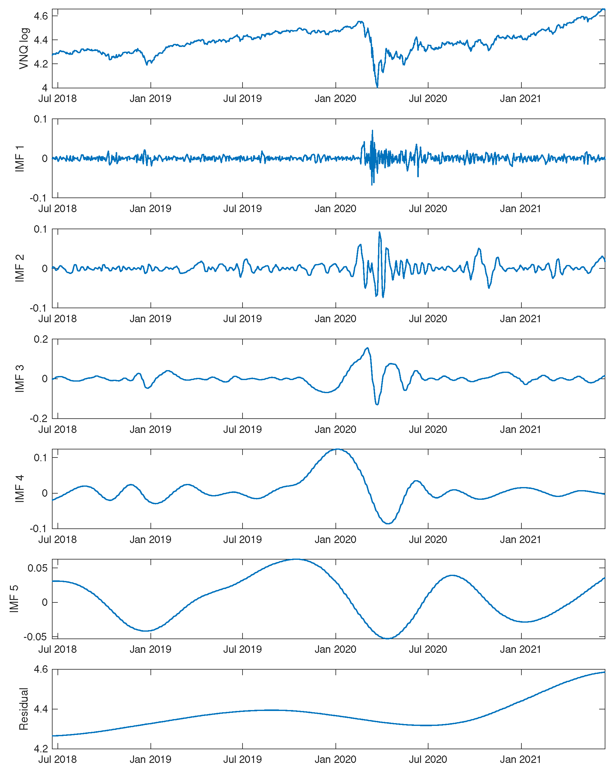
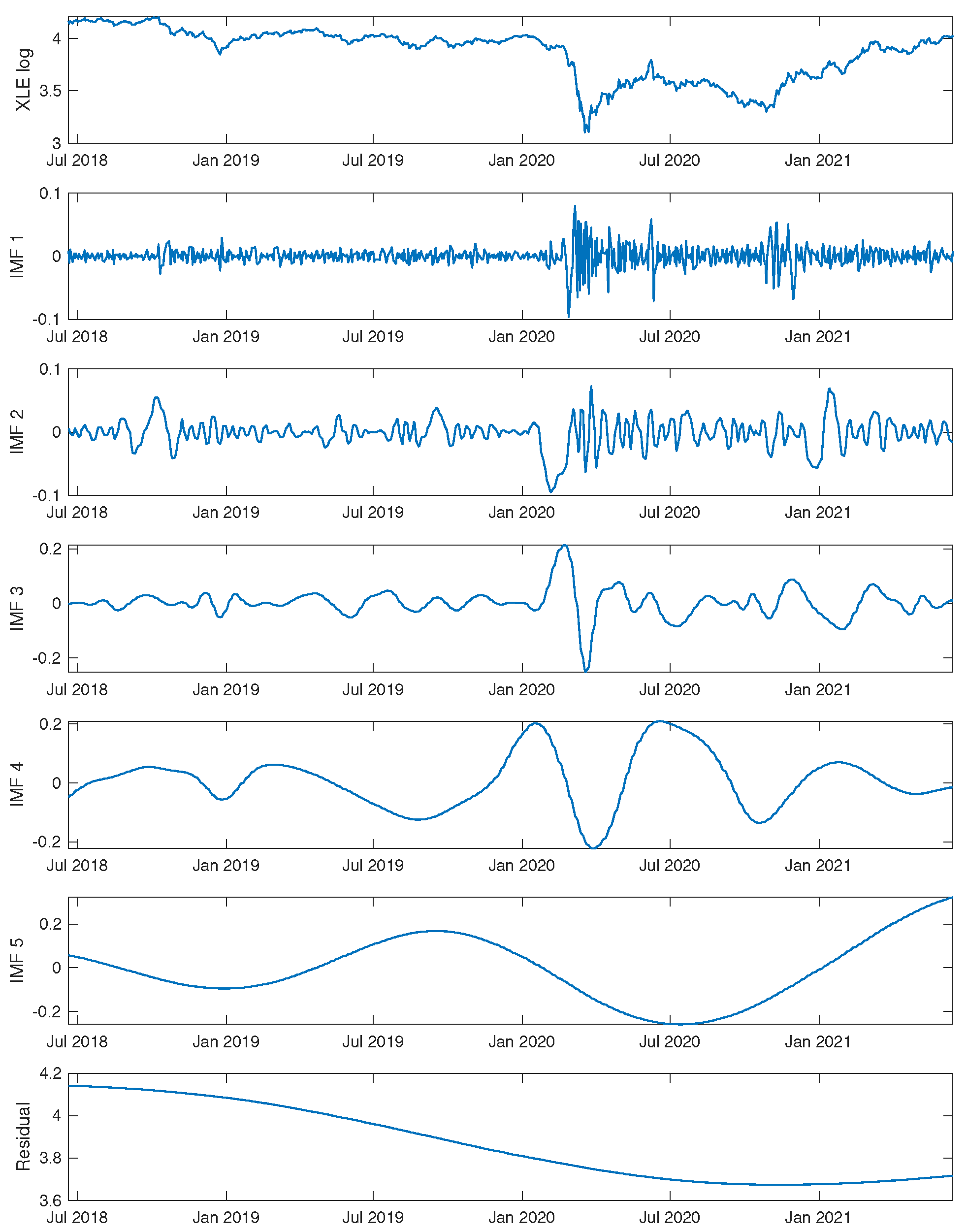
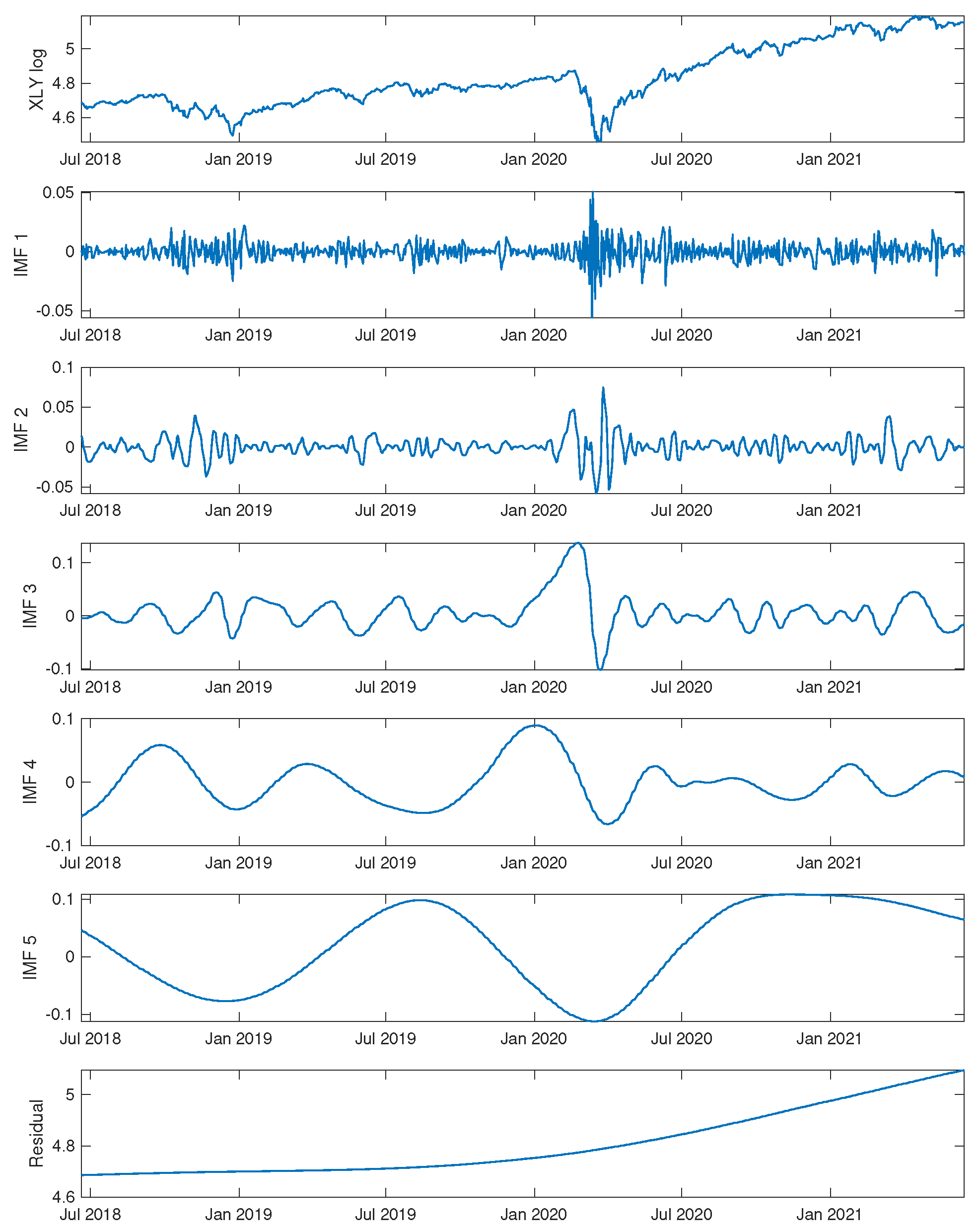
In Figure 1, Figure 2, Figure 3, Figure 4, Figure 5 and Figure 6, we illustrate the decomposition implemented from CEEMD. We take the log prices of the top six sector ETFs: {XLK, XLE, XLF, XLV, XLY, VNQ}, and apply CEEMD to obtain five IMFs along with the residuals. As such, the top row in each plot shows the original log price time series $x(t)$, followed by the IMF $c_j(t)$s with decreasing frequencies, ending with the residual term. The number of IMF components $n=5$, so along with the residual term, there are six components in total. As we can see, the first IMF exhibits the highest frequency of fluctuation, whereas the smooth residual term reflects the overall trend.

The modes on different timescales can indicate different behavior of the time series. Let’s consider the recent COVID-19 event, for example. When S&P 500 and all sector ETFs began the sharp decline from 2/21/2020 on, intrinsic modes 1, 2, and 3 also showed a notable peak around the time period. The lower-frequency modes 4 and 5 exhibited a steep decrease towards the day of market crash.

3. Multiscale Filtering

The CEEMD algorithm is an iterative sifting process that identifies the rapid fluctuations and long-term trends from any given time series. As a consequence, the first few components have higher frequency and the last few components have lower frequency, and they all sum up to the original time series. Hence, by combining different components from the decomposition, CEEMD can be used as a filtering and reconstruction tool.

In the reconstruction of the original time series using the IMF components, we can choose a subset of modes as a filter for desired information. By removing the first few high-frequency components, we create a low-pass filter; that is,

$$x_L^{(m_l)}(t)=x(t)-\sum _{j=1}^{n-m_l+1}{c}_j(t).$$

(6)

This reconstruction using only the last few components can serve as a smoothing of the time series. Similarly, we can also build a high-pass filter with

$$x_H^{(m_h)}(t)=\sum _{j=1}^{m_h}{c}_j(t),$$

(7)

which captures the high-frequency local behaviors, and can also be used to estimate volatility.

In each case, the number of components (including the residual term) equals to $m_l$ and $m_h$, respectively. We use $x_L^{(m_l)}(t)$ and $x_H^{(m_h)}(t)$ to denote the low-pass and high-pass filtered reconstruction of $x(t)$ with $m_l$ and $m_h$ components. Note that the low-pass filter and the high-pass filter are complementary to each other when $m_l+m_h=n+1$, where $n+1$ is the total number of components (including the residual term).

To illustrate these filters, we consider four sector ETFs over a 3-year period. For each ETF, let $s(t)$ be the value of the time series and $x(t):=log(s(t))$ be its log price. In each case, CEEMD is applied to the time series $x(t)$ to extract the IMFs and residual.

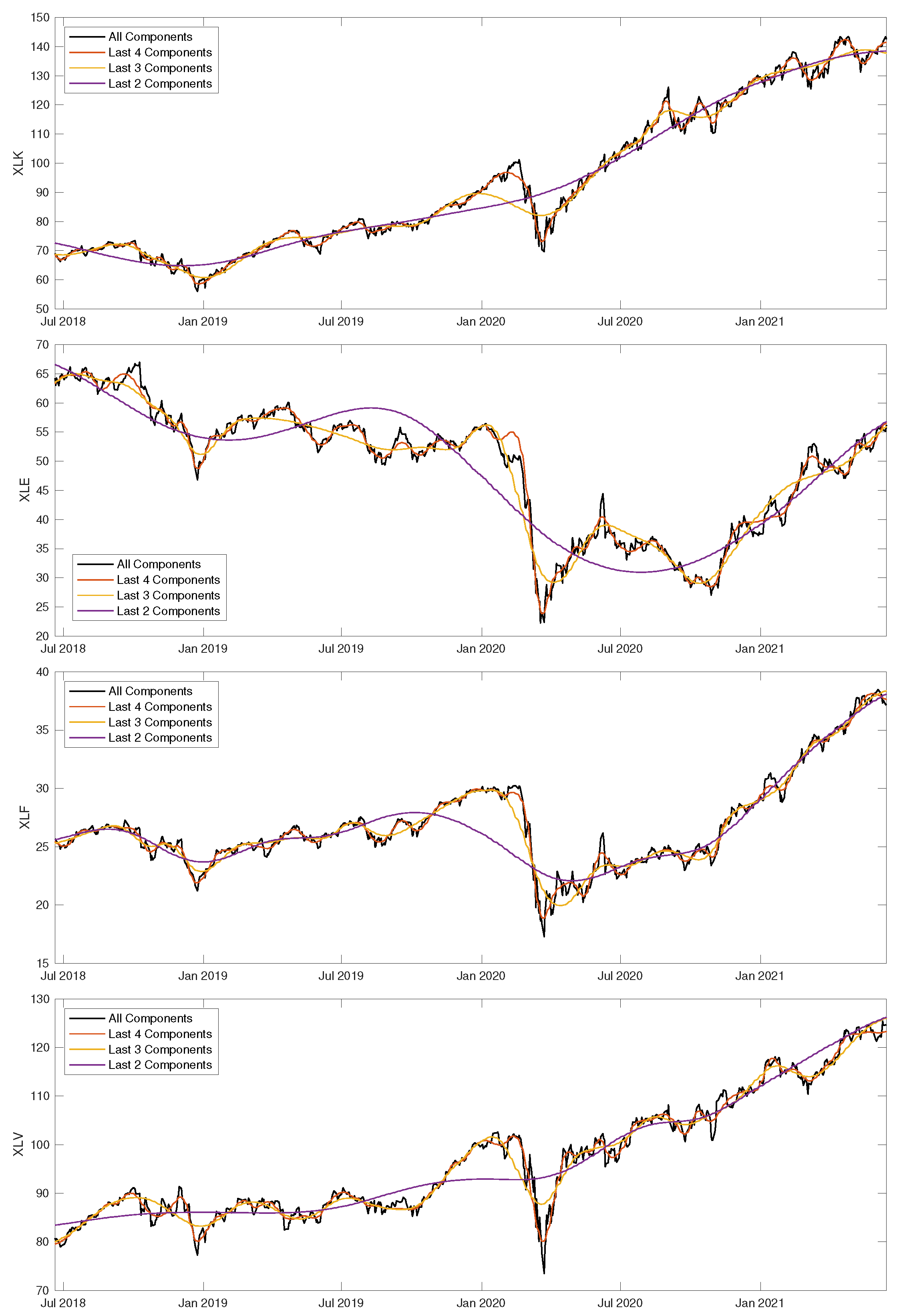
In Figure 7, we show the low-pass filters of the price time series of four sector ETFs: {XLK, XLE, XLF, and XLV}. This involves applying (6) using different collections of components. Specifically, we used the last 4, 3, and 2 components including the residual term, that is, $x_L^{(m_l)}(t)$ with $m_l=4,3,2$. The reconstructed log prices were taken exponentially to approximate the original price data. We can see that, with more components included in the reconstruction, the resulting time series resembles the original time series on a finer timescale. Compared to some other time series smoothing techniques, such as the moving average, the CEEMD low-pass filter achieves smoothing without lags.

4. Multiscale Volatility

We now examine the multiscale properties of volatility we apply CEEMD to filter the original time series into low-pass and high-pass components. Statistical analysis, such as mean and volatility, can be defined on the filtered time series.

4.1. High-/Low-Pass Filters

To set up, let $s(t)$ be the price of the asset price, and $x(t)=logs(t)$ be the log price. Implement CEEMD on $x(t)$ and apply (6) and (7) to get $x_L^{(m_l)}(t)$ and $x_H^{(m_h)}(t)$, with $m_l$ and $m_h$ being the number of components in the low-pass and high-pass filters, respectively. To study the statistical properties of the asset prices, we define the low-pass and high-pass log returns:

$$\begin{array}{cc}\hfill r_L^{(m_l)}(t)& =x_L^{(m_l)}(t)-x_L^{(m_l)}(t-1),\hfill \end{array}$$

(8)

$$\begin{array}{cc}\hfill r_H^{(m_h)}(t)& =x_H^{(m_h)}(t)-x_H^{(m_h)}(t-1).\hfill \end{array}$$

(9)

The low-pass volatility and high-pass volatility are the standard deviation of the low-pass and high-pass returns, defined by the unbiased estimators

$$\begin{array}{cc}\hfill {\sigma }_L^{(m_l)}& =\sqrt{\frac{1}{T-1}{\sum }_{t=1}^T{\left(r_L^{(m_l)}(t)-{\mu }_L^{(m_l)}\right)}^2},\hfill \end{array}$$

(10)

$$\begin{array}{cc}\hfill {\sigma }_H^{(m_h)}& =\sqrt{\frac{1}{T-1}{\sum }_{t=1}^T{\left(r_H^{(m_h)}(t)-{\mu }_H^{(m_h)}\right)}^2},\hfill \end{array}$$

(11)

where

$${\mu }_L^{(m_l)}=\frac{1}{T}\sum _{t=1}^T{r}_L^{(m_l)}(t),{\mu }_H^{(m_h)}=\frac{1}{T}\sum _{t=1}^T{r}_H^{(m_h)}(t)$$

(12)

are the mean low-pass and high-pass log returns.

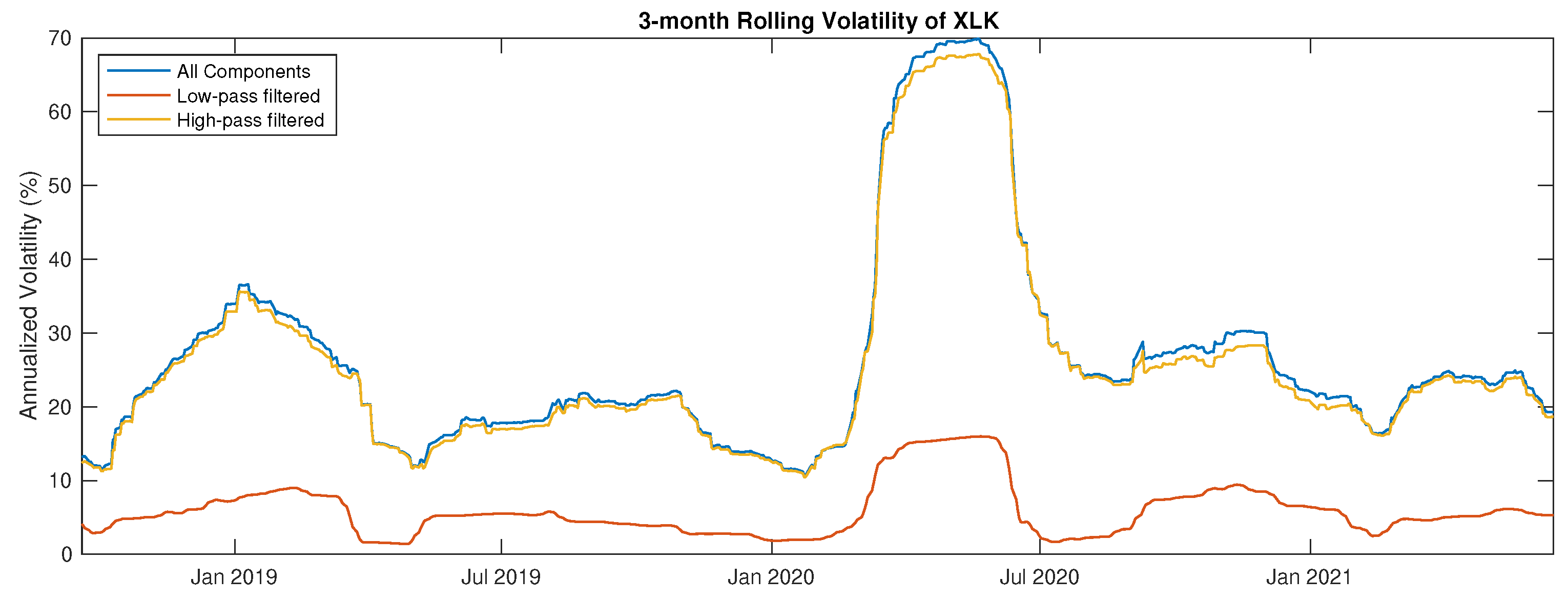
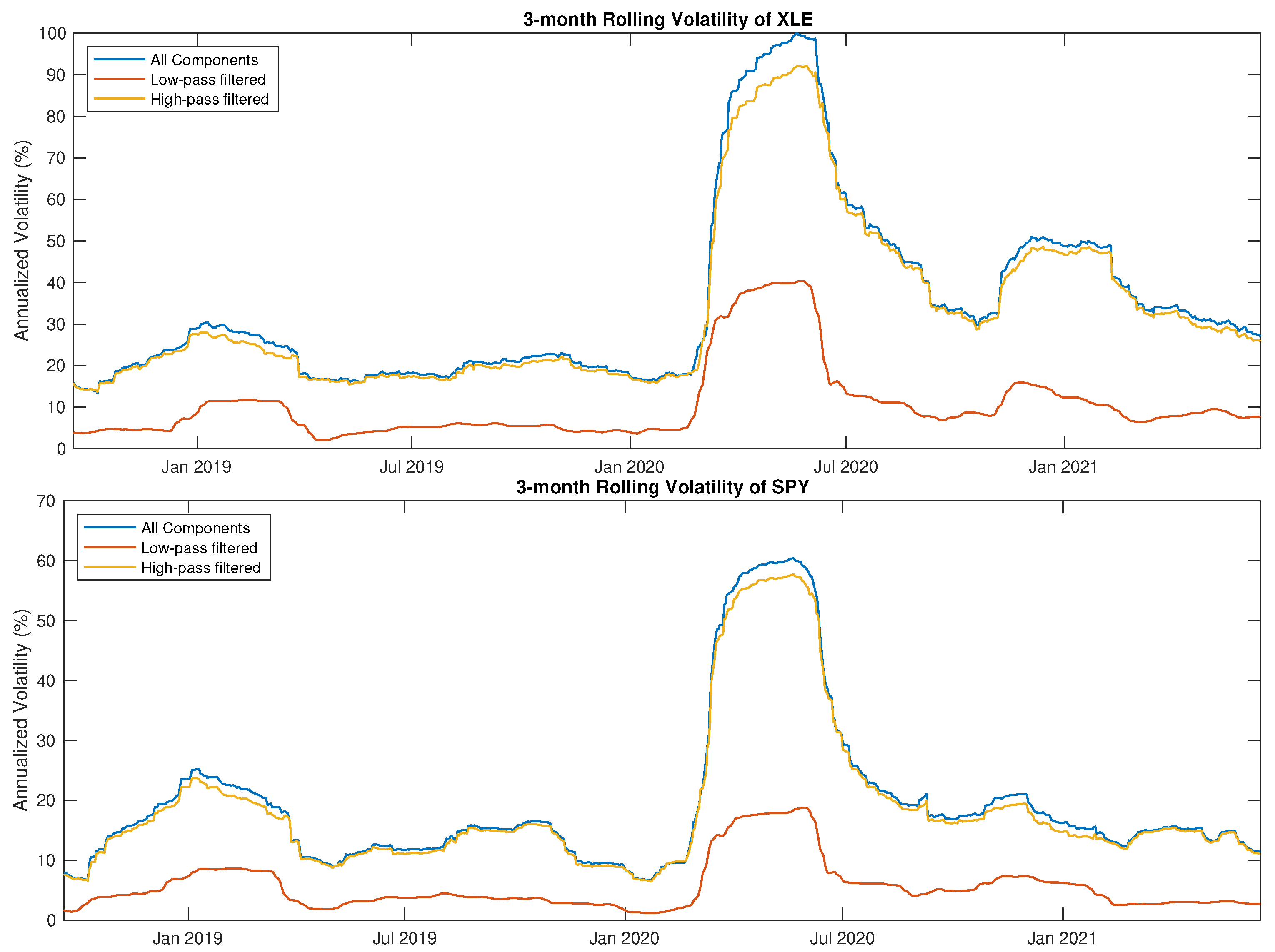
Figure 8 and Figure 9 show the 3-month rolling volatility of XLK, XLE, and SPY computed using all components, high-pass filtered data, and low-pass filtered data. Recall from Figure 1 and Figure 6 that the time series are decomposed into six components, including the residual terms. We use $m_l=4$ for low-pass filtering and $m_h=2$ for high-pass filtering. Notice that the high-pass filtered time series captures most of the volatility residing in the original times series. This is also observed in

Table 2. Percentage of log return variance in IMF component reconstruction of sector ETFs (%).

	First 5	First 4	First 3	First 2	First 1	Last 5	Last 4	Last 3	Last 2	Last 1
XLK	99.8259	99.6508	98.5317	92.9884	77.3954	19.7625	6.0245	1.0859	0.2588	0.0054
XLE	99.6452	99.1981	95.3561	87.5555	71.9705	25.5809	12.9790	3.6628	0.9244	0.0451
XLF	99.4613	98.8796	96.4074	90.2359	72.9261	25.2204	8.8075	2.7549	0.7481	0.4160
XLV	99.8574	99.6924	97.5934	92.6984	73.0258	25.3905	6.8497	1.5566	0.1210	0.0711
XLY	99.7793	99.4109	97.6389	89.9345	68.9575	26.6930	8.6944	1.6817	0.7732	0.0686
XLP	99.8637	99.5129	98.5454	92.1821	71.2906	23.5865	7.0254	1.0266	0.3154	0.0118
XLI	99.7285	99.3705	97.1640	89.5023	69.6809	27.4544	9.0584	2.3807	0.6726	0.1157
XLB	99.6872	99.2413	97.1382	90.0120	66.0320	30.7538	9.3170	2.4662	0.5770	0.1226
XLU	99.8460	99.7146	99.0680	92.3583	71.5283	24.3641	7.0881	0.8368	0.1555	0.0280
XLC	99.7025	99.5082	98.6954	92.1340	75.4771	22.4029	7.2018	0.8245	0.2376	0.1101
VNQ	99.6289	99.2716	98.2043	89.1387	68.9805	28.0985	9.4033	1.3126	0.5772	0.1554
SPY	99.7060	99.4936	97.7869	90.4462	71.7355	24.8835	9.4217	1.7540	0.4948	0.2072

. Hence, we consider using the stationary high-pass filtered data for statistical analysis.

4.2. Volatility Asymmetry

It has been observed in the financial market that the volatility of asset returns is usually asymmetric, that is, the volatility is higher in a downside market than that in an upside market. Following Bekaert and Wu (2000), we capture the asymmetry by looking at the conditional volatility. Specifically, we examine whether the asymmetry exists in the price dynamics. To that end, we define the conditional volatilities based on the ACE-EMD high-pass filter as follows:

$$\begin{array}{c}\hfill {\sigma }_{+H}^{(m_h)}=\sqrt{Var(r_H^{(m_h)}(t)|r_H^{(m_h)}(t-1)>{\mu }_H^{(m_h)})},\end{array}$$

(13)

$$\begin{array}{c}\hfill {\sigma }_{-H}^{(m_h)}=\sqrt{Var(r_H^{(m_h)}(t)|r_H^{(m_h)}(t-1)<{\mu }_H^{(m_h)})}.\end{array}$$

(14)

In essence, ${\sigma }_{+H}^{(m_h)}$ and ${\sigma }_{-H}^{(m_h)}$ capture the high-pass volatilities conditioned on an upside movement and a downside movement, respectively.

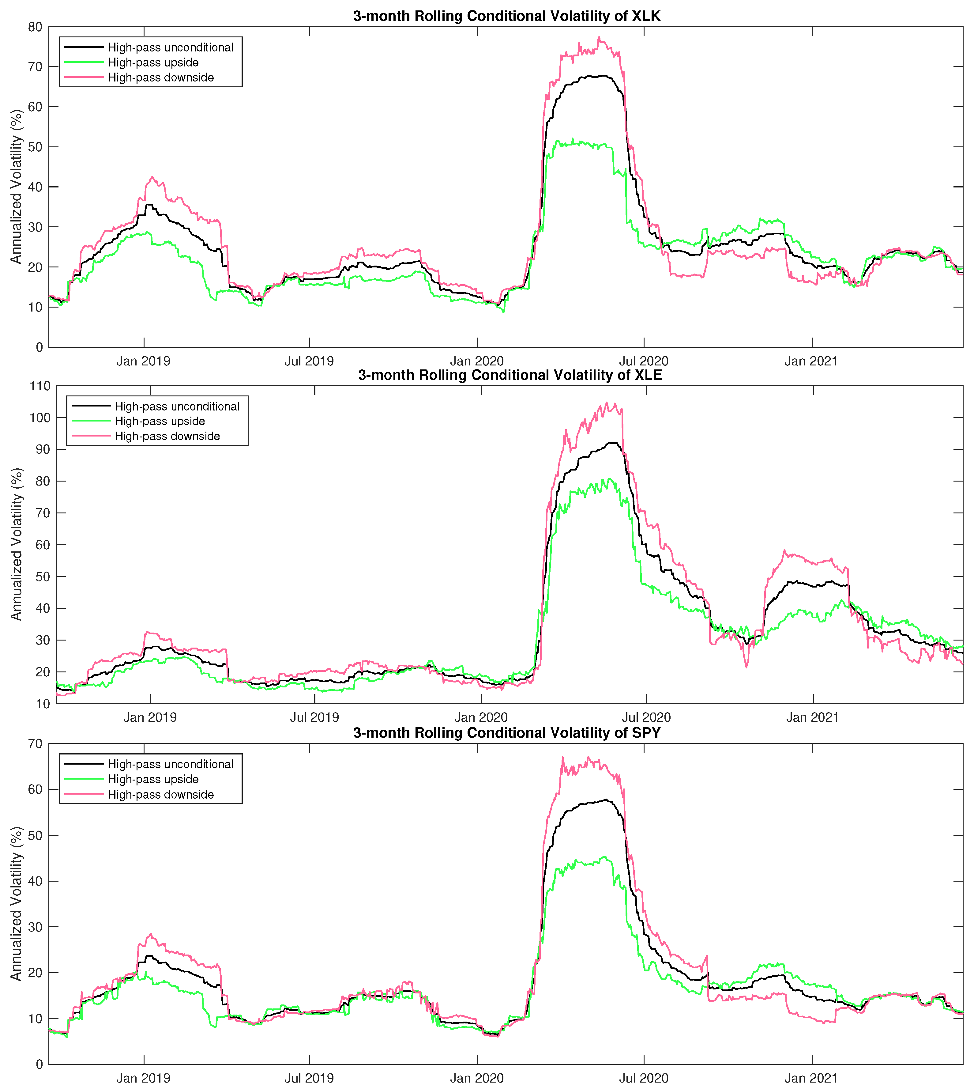
Figure 10 shows the 3-month rolling estimation of the conditional volatility using high-pass filtered data of XLK, XLE, and SPY. In the high-pass components, we see that S&P 500 shows asymmetric volatility with a larger downside volatility most of the time. The sector ETFs, however, exhibit both directions of asymmetry, where upside and downside movements trigger high volatility alternately during different periods of time. This phenomenon suggests distinct behavior of the sector ETFs comparing with the traditional equity indices.

Define the events of upside volatility asymmetry and downside volatility asymmetry as:

$$A^{+}=({\sigma }_{+H}^{(m_h)}-{\sigma }_{-H}^{(m_h)})>ϵ{\sigma }_H^{(m_h)}$$

(15)

$$A^{-}=({\sigma }_{+H}^{(m_h)}-{\sigma }_{-H}^{(m_h)})<-ϵ{\sigma }_H^{(m_h)}$$

(16)

In Figure 11, we plot the frequency of event $A^{+}$, as defined in (15), against the frequency of event $A^{-}$, as defined in (16). The dashed line corresponds to $\mathbb{P}(A^{+})+\mathbb{P}(A^{-})=1$, and the closeness to the dashed line indicates the level of volatility asymmetry in general. We can see there are clear clusters separating the ETFs. In the upper left region, the corresponding ETFs, such as XLP, XLY, and XLC, are upside volatility asymmetry dominated. In contrast, towards the lower right direction the corresponding ETFs are downside volatility asymmetry dominated. The sector ETFs with the highest probability of downside asymmetry are XLU, XLE, XLK, XLV, and XLB. The S&P 500 index ETF, along with XLF and XLI, lie somewhere in the middle in terms of the upside/downside asymmetry.

5. Energy-Frequency Spectrum

As is well-known (see Koopmans 1995; Huang et al. 2003, among others), spectral analysis provides an alternative aspect to analyze time series on the frequency domain. The definition of an IMF is very amenable to Hilbert spectral analysis. In this section, we apply this approach to compute and analyze the energy-frequency spectra of the sector ETFs.

5.1. Hilbert Spectral Analysis

Every oscillating real-valued function can be viewed as the projection of an orbit on the complex plane onto the real axis. For any function in time $X(t)$, the Hilbert transform is given by

$$Y(t)=\mathcal{H}\left[X\right](t):=\frac{1}{\pi }{\int }_{-\infty }^{+\infty }\frac{X(s)}{t-s}ds,$$

(17)

where the improper integral is defined as the Cauchy principle value. The transform exists for any function in $L^p$ (see Titchmarsh 1948). As a result, $Y(t)$ provides the complementary imaginary part of $X(t)$ to form an analytic function in the upper half-plane defined by

$$Z(t)=X(t)+iY(t)=a(t)e^{i\theta (t)},$$

(18)

where

$$\begin{array}{cc}\hfill a(t)& =\parallel Z(t)\parallel =\sqrt{X^2(t)+Y^2(t)},\hfill \end{array}$$

(19)

$$\begin{array}{cc}\hfill \theta (t)& =argZ(t)=arctan(\frac{Y(t)}{X(t)}).\hfill \end{array}$$

(20)

Recall from Equation (2) that an IMF admits the form $c(t)=a(t)cos(\theta (t))$. It is known that if the amplitude and frequency are slow modulations, then the corresponding Hilbert transform gives a $\pi /2$ shift to the phase $\theta (t)$ (see Bedrosian 1963; Nuttall and Bedrosian 1966). Therefore, the $a(t)$ given by (19) is the instantaneous amplitude, and the $\theta (t)$ given by (20) is the instantaneous phase function. The instantaneous frequency is then defined as the $2\pi$-standardized rate of change of the phase function:

$$f(t)=\frac{1}{2\pi }\dot{\theta }(t)=\frac{1}{2\pi }\frac{d}{dt}\left(arctan(\frac{Y(t)}{X(t)})\right).$$

(21)

Applying Hilbert transform to each of the IMF components individually yields a sequence of analytic signals (see Huang et al. 1998):

$$c_j(t)+i\mathcal{H}\left[c_j\right](t)=a_j(t)e^{i{\theta }_j(t)},$$

(22)

for $j=1,\cdots ,n$. In turn, the original time series can be represented as

$$x(t)=\mathfrak{Re}\sum _{j=1}^n{a}_j(t)e^{i{\int }^{t}2\pi f_j(s)ds}+r_n(t).$$

(23)

This decomposition can be seen as a sparse spectral representation of the time series with time-varying amplitude and frequency. In other words, each IMF represents a generalized Fourier expansion that are suitable for nonlinear and nonstationary financial time series. In summary, the procedure generates a series of complex functions that are analytic in time, along with their associated instantaneous amplitudes and instantaneous frequencies. These components capture different time scales and resolutions embedded in the time series and are used for time series filtering and reconstruction.

Lastly, the Hilbert spectrum is defined by

$$H(f,t)=\sum _{j=1}^n{H}_j(f,t),\mathrm{where}{\displaystyle H_j(f,t)=\left\{\begin{array}{cc}{a}_j(t),\hfill & f=f_j(t),\hfill \\ 0,\hfill & \mathrm{otherwise}.\hfill \end{array}\right.}$$

(24)

The instantaneous energy of the j-th component is defined as

$$E_j(t)={\left|a_j(t)\right|}^2.$$

(25)

We examine the behavior of the Hilbert spectrum through the pair $(f_j(t),E_j(t))$ for $t\in [0,T]$ and $j=1,\cdots ,n$ (see Figure 12), which forms a sparse energy-frequency spectrum. Through this new lens, we examine the behaviors of the time series.

5.2. Central Frequency and Power Spectrum

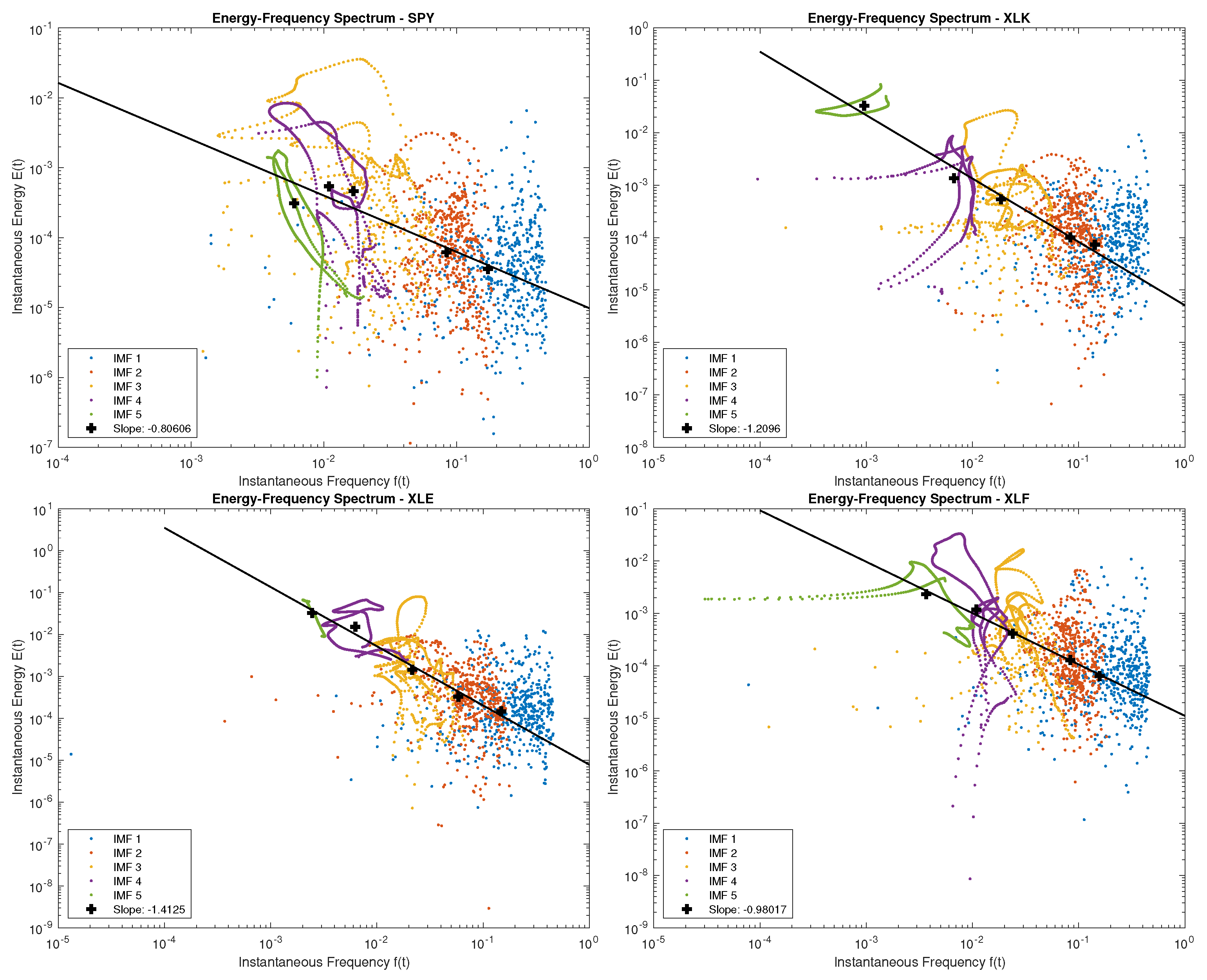
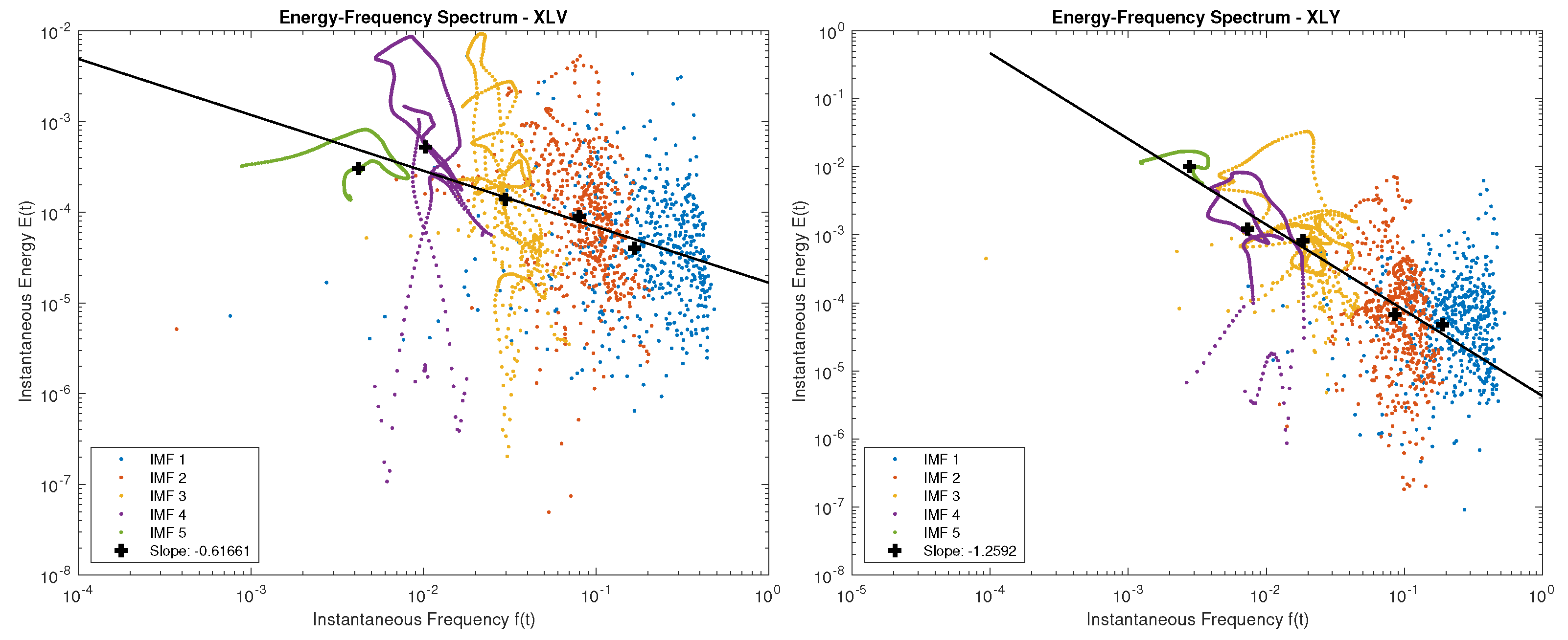
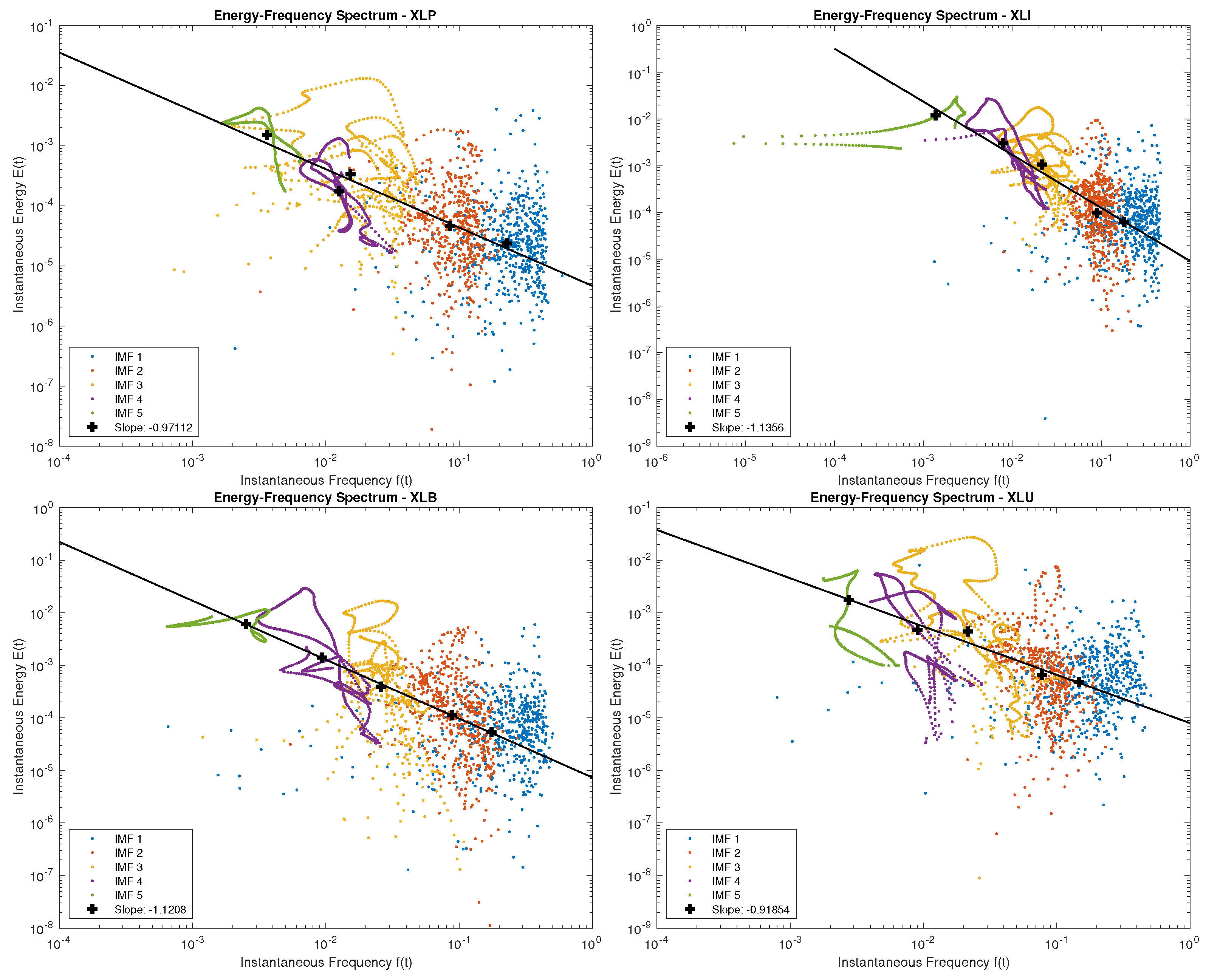
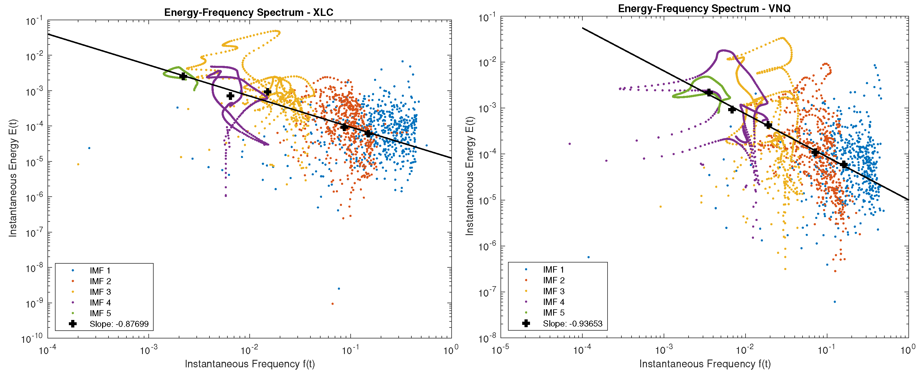
For each time series, we can obtain the instantaneous frequency $f_j(t)$ from (21) and instantaneous energy $E_j(t)$ from (25), corresponding to mode $j=1,\cdots ,n$. This allows us to derive the instantaneous energy-frequency spectrum as shown in Figure 12, Figure 13, Figure 14 and Figure 15. Each point on the plots is a pair of $(f_j(t),E_j(t))$, for mode $j=1,\cdots ,n$, and time $t=1,\cdots ,T$. We see that for each mode j, the instantaneous energy-frequency pairs $(f_j(t),E_j(t)),t=1,\cdots ,T$ form a cluster of points. We define the central frequency and central energy of mode j during the time period $[0,T]$ as follows:

$$\begin{array}{cc}\hfill {\overline{f}}_j& =exp\left(\frac{1}{T}{\int }_0^{T}log{f}_j(t)dt\right),\hfill \end{array}$$

(26)

$$\begin{array}{cc}\hfill {\overline{E}}_j& =exp\left(\frac{1}{T}{\int }_0^{T}log{E}_j(t)dt\right).\hfill \end{array}$$

(27)

While the instantaneous frequency and energy are time-varying, they are typically fluctuating or orbiting around the central points. Dragomiretskiy and Zosso (2013) assumed a central frequency in each mode and used the concept to derive the variational mode decomposition (VMD). Intuitively, the central frequency and central energy capture the overall spectral properties of the time series (see Wu and Huang 2004).

From Figure 12, Figure 13, Figure 14 and Figure 15 we also observe a clear linear relationship in the log space of central frequency and energy pair $({\overline{f}}_j,{\overline{E}}_j)$, which are marked as the black crosses. A linear regression is run on the central frequencies to estimate the slope of the spectrum. This indicates a power spectrum relation

$$E(f)\sim \frac{1}{f^{\alpha }}.$$

(28)

The power spectrum exponent $\alpha$ controls how fast the energy decays from lower to higher frequency, and is key to the property of the spectrum and the associated time series. It has been long observed that many time series in nature have $\alpha$ close to one, well-known as the $1/f$ spectrum or “pink noise”. In Figure 12, Figure 13, Figure 14 and Figure 15, the solid line in each plot is obtained from linear regression of $(log({\overline{f}}_j),log({\overline{E}}_j))$. The negative slope of the line estimates the power spectrum exponent $\alpha$ for the time series. The power spectrum exponents for the S&P 500 index and U.S. sector ETFs are summarized in

Table 3. Power spectrum exponents for the S&P 500 index and U.S. sector ETFs.

ETF	$\mathit{\alpha }$	ETF	$\mathit{\alpha }$	ETF	$\mathit{\alpha }$
SPY	0.8000	XLK	1.2001	XLE	1.4110
XLF	0.9785	XLV	0.6146	XLY	1.2625
XLP	0.9729	XLI	1.1377	XLB	1.1059
XLU	0.9204	XLC	0.8836	VNQ	0.9265

.

5.3. Frequency Synchronization

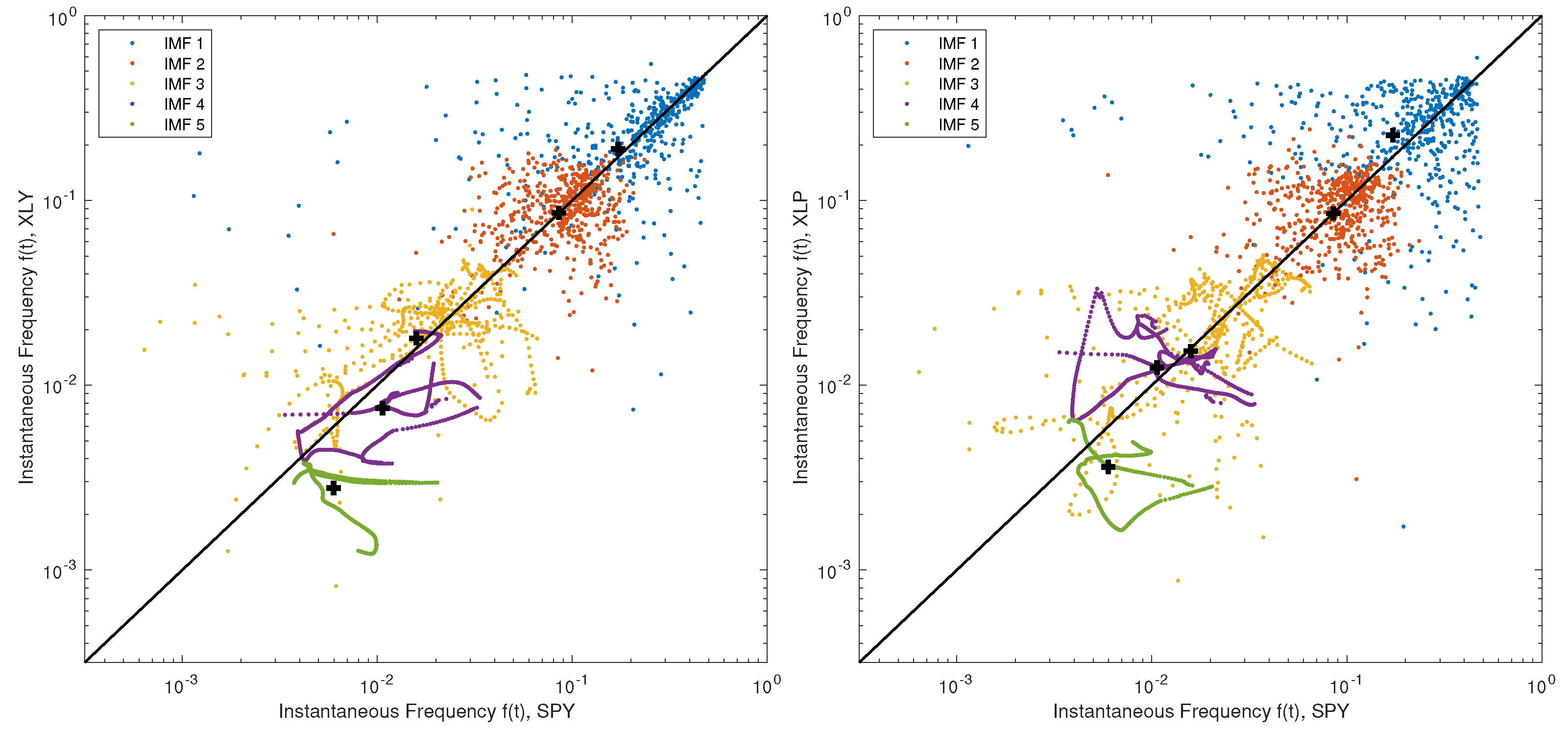
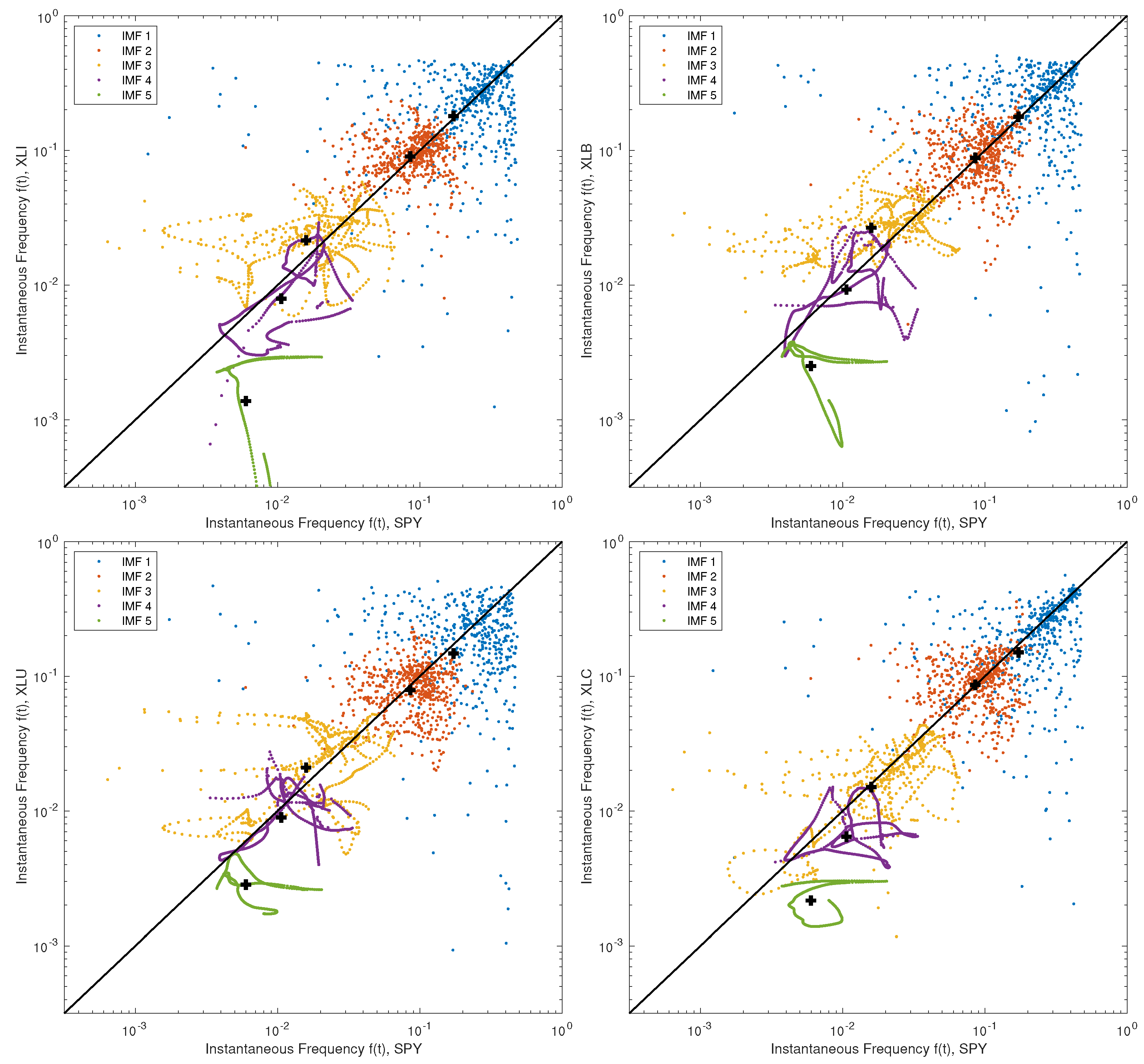
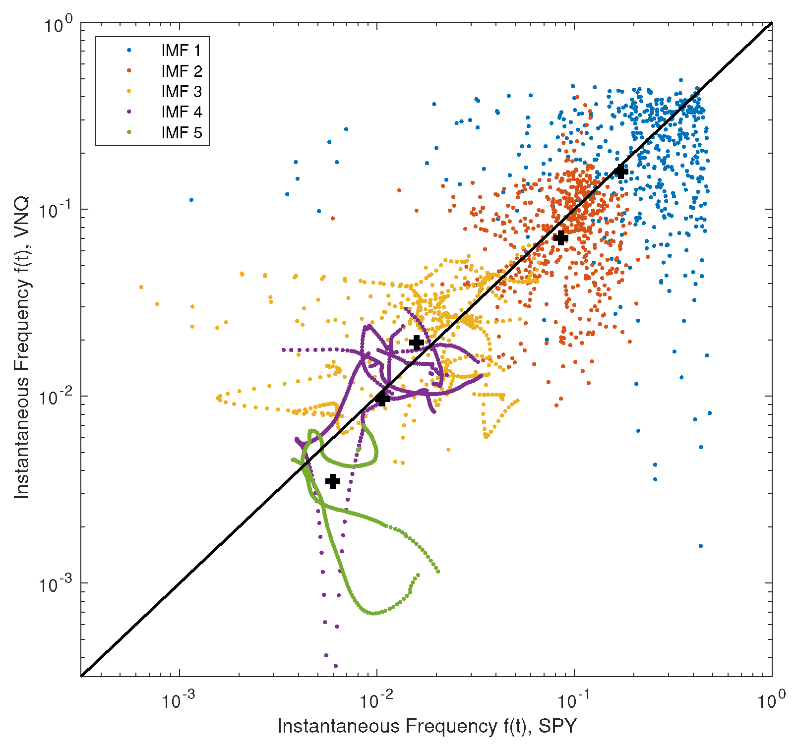
To further investigate the spectral characteristics of sector ETFs, we conduct a pair-wise comparison between each sector ETF and the S&P500 ETF (SPY). For each pair of ETFs, we plot the associated central frequencies derived from their price time series, denoted by ${\overline{f}}_j,j=1,\cdots ,n$. In Figure 16, Figure 17, Figure 18 and Figure 19, we show the log-log scatter plots of the instantaneous frequencies of sector ETFs and SPY. Each point on the plot is a pair of instantaneous frequencies of the two time series recorded at the same time, and the central frequencies are marked as black crosses. The solid straight line of unit slope shows the reference line for identical frequencies.

We observe that some sector ETFs, such as XLF and VNQ, appear to share similar frequency profiles and their central frequencies are very close. On the other hand, the central frequencies deviate from the identical line at low-frequency modes for all sector ETFs vs. SPY, with XLK being the most extreme example. This means that sector ETFs tend to exhibit slower dynamics in the longer term components, while the fast modes of both sector ETFs and SPY have similar mean frequencies. Similar frequency profiles suggest synchronization, which is a typical phenomenon in nonlinear dynamics with interaction (see e.g., Pikovsky et al. 2003). In order to quantify the frequency synchronization level between two time series $x_1$ and $x_2$, we define the associated frequency deviation as follows:

$$D(x_1,x_2):=\sum _{j=1}^n{log}^2\left(\frac{{\overline{f}}_j^{(1)}}{{\overline{f}}_j^{(2)}}\right)={\parallel log({\overline{f}}^{(1)})-log({\overline{f}}^{(2)})\parallel }^2.$$

(29)

A lower frequency deviation value represents a higher synchronization level. In particular, we have $D(x_1,x_2)=0$ if, and only if the central frequencies of all the IMF components are identical for $x_1$ and $x_2$, meaning the two time series are fully synchronized.

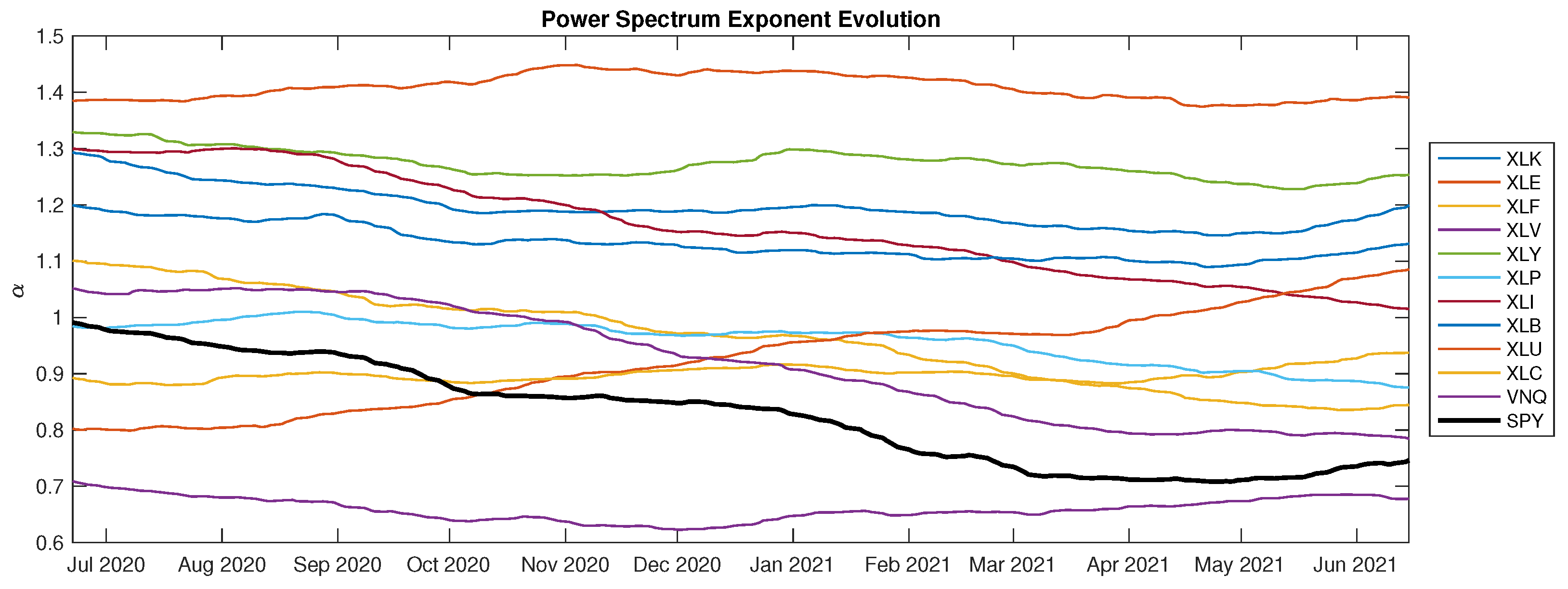
To see how the sector ETFs have evolved compared to the S&P 500, we plot their power spectrum exponent $\alpha$ estimated from a 2-year rolling window. As shown in Figure 20, the power spectrum exponents $\alpha$ of most sector ETFs are consistently higher than that of SPY. Over the one-year period, the power spectrum exponent of SPY is gradually decreasing from close to 1 to less than 0.8. Several sector ETFs, such as XLE and XLY, continue to have the highest power spectrum exponents through time. In contrast, the real estate ETF VNQ is seen to have the lowest power spectrum exponent over time.

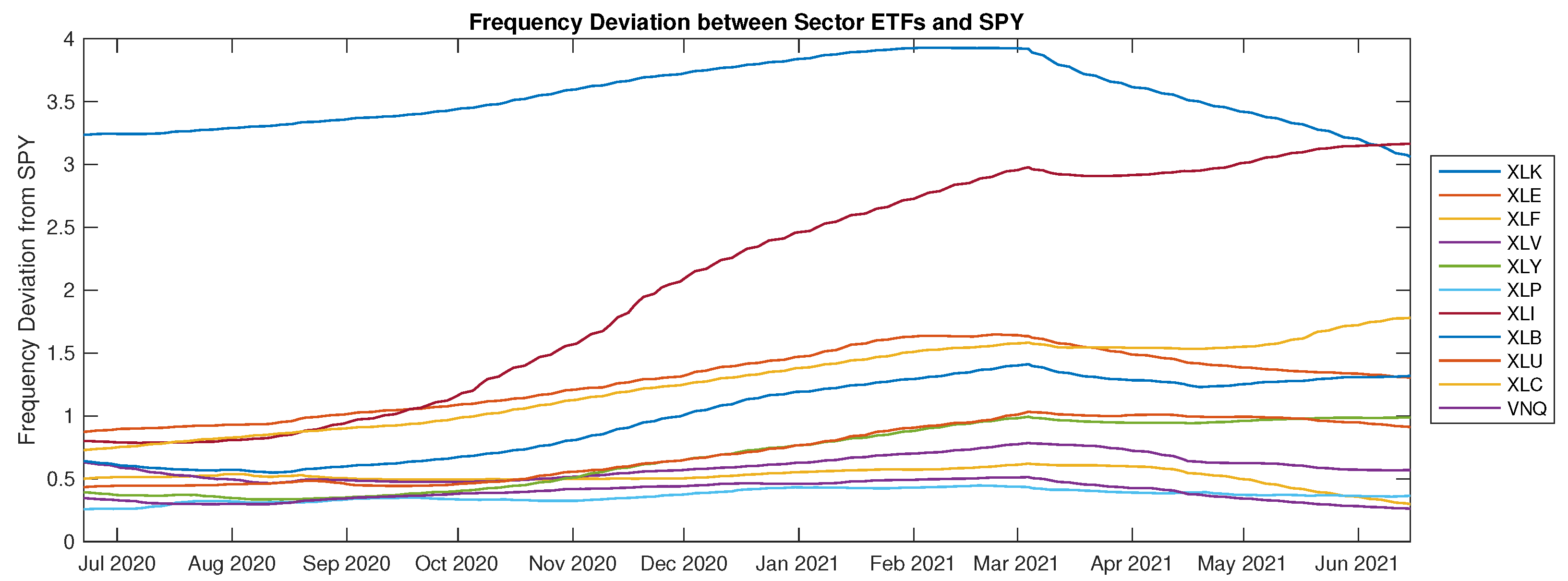
Furthermore, in Figure 21, we see that the sector ETF frequency deviation, when compared against SPY as defined in (29), has shown a general trend of increase from 2020 to 2021. The largest frequency deviation comes from the technology ETF XLK, while the industrial sector ETF XLI has experienced a drastic continual increase in frequency deviation. These observations are evidence of partial asynchronization over a relatively long period of time.

The power spectra and frequency profiles provide new perspectives on how to differentiate and compare the price dynamics of sector ETFs. Our findings on these ETFs are useful for a number of practical purposes, including sector rotation, asset allocation, and portfolio diversification, which are vital not only for individual and institutional investors. Our study also discovers some new price behaviors and properties of sector ETFs. The multiscale metrics used herein, such as asymmetric volatility and frequency deviation, provide better understanding of the risks associated with these ETFs, which is important for both investors and policy makers.

6. Conclusions

We developed a data-driven algorithm to discover and examine the multiscale characteristics of U.S. sector ETF price dynamics, including intrinsic mode functions of various frequencies. Different combinations of modes allow us to filter the financial time series or estimate its volatility based on different timescales. Across all sector ETFs, we compare their price behaviors as well as multiscale properties. In the same spirit, we apply Hilbert spectral analysis to compute the associated instantaneous energy-frequency spectrum for each sector ETF. In particular, the power spectrum exponents of most sector ETFs have been significantly higher than that of the S&P 500, and the phenomenon tends to persist.

The EMD approach also has its shortcomings. One common issue is the end-effect, whereby the decomposition becomes less accurate near both ends of the time series (see Chen and Feng 2003, among others). The noise-assisted CEEMD method here partially addresses the end effect, but there is no guarantee. In addition, the number of modes from EMD may depend on a number of factors, such as the time frame of the data. Therefore, if two time series result in different numbers of modes, then comparison becomes less direct. As a remedy, one can pre-specify a common number of modes for the decomposition of multiple time series.

For future research, one direction is to apply or extend CEEMD to examine the high-frequency price evolution of ETFs and other assets. The CEEMD method can also be used to generate a collection of new HHT features. These features can be integrated into machine learning models, leading to several practical applications, such as forecasting and classification (see e.g., Leung and Zhao 2021b).

References

- Aloui, Chaker, Syed Jawad Hussain Shahzad, and Rania Jammazi. 2018. Dynamic efficiency of european credit sectors: A rolling-window multifractal detrended fluctuation analysis. Physica A: Statistical Mechanics and Its Applications 506: 337–49. [Google Scholar] [CrossRef]
- Arugaslan, Onur, and Ajay Samant. 2014. Evaluating s&p 500 sector etfs using risk-adjusted performance measures. Journal of Finance, Accounting and Management 5: 48. [Google Scholar]
- Bedrosian, Edward. 1963. A product theorem for Hilbert transforms. Proceedings of the IEEE 51: 868–69. [Google Scholar] [CrossRef]
- Bekaert, Geert, and Guojun Wu. 2000. Asymmetric volatility and risk in equity markets. The Review of Financial Studies 13: 1–42. [Google Scholar] [CrossRef] [Green Version]
- Chen, Yangbo, and Maria Q. Feng. 2003. A technique to improve the empirical mode decomposition in the hilbert-huang transform. Earthquake Engineering and Engineering Vibration 2: 75–85. [Google Scholar] [CrossRef] [Green Version]
- Dragomiretskiy, Konstantin, and Dominique Zosso. 2013. Variational mode decomposition. IEEE Transactions on Signal Processing 62: 531–44. [Google Scholar] [CrossRef]
- Fouque, Jean-Pierre, George Papanicolaou, Ronnie Sircar, and Knut Solna. 2003. Multiscale stochastic volatility asymptotics. Multiscale Modeling & Simulation 2: 22–42. [Google Scholar]
- Hou, Thomas Y., and Zuoqiang Shi. 2011. Adaptive data analysis via sparse time-frequency representation. Advances in Adaptive Data Analysis 3: 1–28. [Google Scholar] [CrossRef]
- Hou, Thomas Y., and Zuoqiang Shi. 2013. Data-driven time-frequency analysis. Applied and Computational Harmonic Analysis 35: 284–308. [Google Scholar] [CrossRef]
- Hou, Thomas Y., Mike P. Yan, and Zhaohua Wu. 2009. A variant of the EMD method for multi-scale data. Advances in Adaptive Data Analysis 1: 483–516. [Google Scholar] [CrossRef] [Green Version]
- Huang, Boqiang, and Angela Kunoth. 2013. An optimization based empirical mode decomposition scheme. Journal of Computational and Applied Mathematics 240: 174–83. [Google Scholar] [CrossRef]
- Huang, Norden Eh. 2014. Hilbert-Huang Transform and Its Applications. Interdisciplinary Mathematical Sciences: vol. 16. Singapore: World Scientific. [Google Scholar]
- Huang, Norden Eh, Man-Li Wu, Wendong Qu, Steven R. Long, and Samuel SP Shen. 2003. Applications of Hilbert–Huang transform to non-stationary financial time series analysis. Applied Stochastic Models in Business and Industry 19: 245–68. [Google Scholar] [CrossRef]
- Huang, Norden Eh, Zheng Shen, and Steven R. Long. 1999. A new view of nonlinear water waves: The Hilbert spectrum. Annual Review of Fluid Mechanics 31: 417–57. [Google Scholar] [CrossRef] [Green Version]
- Huang, Norden Eh, Zheng Shen, Steven R. Long, Manli C. Wu, Hsing H. Shih, Quanan Zheng, Nai-Chyuan Yen, Chi Chao Tung, and Henry H. Liu. 1998. The empirical mode decomposition and the Hilbert spectrum for nonlinear and non-stationary time series analysis. Proceedings of the Royal Society of London. Series A: Mathematical, Physical and Engineering Sciences 454: 903–95. [Google Scholar] [CrossRef]
- In, Francis, and Sangbae Kim. 2012. An Introduction to Wavelet Theory in Finance. Singapore: World Scientific. [Google Scholar] [CrossRef]
- Koopmans, Lambert H. 1995. The Spectral Analysis of Time Series. Oxford: Academic Press. [Google Scholar]
- Leung, Tim, and Theodore Zhao. 2021a. Adaptive complementary ensemble emd and energy-frequency spectra of cryptocurrency prices. International Journal of Financial Engineering 8: 2141008. [Google Scholar] [CrossRef]
- Leung, Tim, and Theodore Zhao. 2021b. Financial time series analysis and forecasting with HHT feature generation and machine learning. Applied Stochastic Models in Business and Industry. [Google Scholar] [CrossRef]
- Li, Jing, Cai Liu, Zhaofa Zeng, and Lingna Chen. 2015. GPR signal denoising and target extraction with the CEEMD method. IEEE Geoscience and Remote Sensing Letters 12: 1615–19. [Google Scholar]
- Maghyereh, Aktham I., Basel Awartani, and Hussein Abdoh. 2019. The co-movement between oil and clean energy stocks: A wavelet-based analysis of horizon associations. Energy 169: 895–913. [Google Scholar] [CrossRef]
- Mensi, Walid, Aviral Kumar Tiwari, and Seong-Min Yoon. 2017. Global financial crisis and weak-form efficiency of islamic sectoral stock markets: An mf-dfa analysis. Physica A: Statistical Mechanics and Its Applications 471: 135–46. [Google Scholar] [CrossRef]
- Nava, Noemi, Tiziana Di Matteo, and Tomaso Aste. 2018a. Dynamic correlations at different time-scales with empirical mode decomposition. Physica A: Statistical Mechanics and Its Applications 502: 534–44. [Google Scholar] [CrossRef]
- Nava, Noemi, Tiziana Di Matteo, and Tomaso Aste. 2018b. Financial time series forecasting using empirical mode decomposition and support vector regression. Risks 6: 7. [Google Scholar] [CrossRef] [Green Version]
- Niu, Mingfei, Yufang Wang, Shaolong Sun, and Yongwu Li. 2016. A novel hybrid decomposition-and-ensemble model based on CEEMD and GWO for short-term PM2.5 concentration forecasting. Atmospheric Environment 134: 168–80. [Google Scholar] [CrossRef]
- Nuttall, A. H., and Edward Bedrosian. 1966. On the quadrature approximation to the Hilbert transform of modulated signals. Proceedings of the IEEE 54: 1458–59. [Google Scholar] [CrossRef]
- Pikovsky, Arkady, Jurgen Kurths, Michael Rosenblum, and Jürgen Kurths. 2003. Synchronization: A Universal Concept in Nonlinear Sciences. Cambridge: Cambridge University Press, vol. 12. [Google Scholar]
- Rilling, Gabriel, Patrick Flandrin, and Paulo Goncalves. 2003. On empirical mode decomposition and its algorithms. In IEEE-EURASIP Workshop on Nonlinear Signal and Image Processing. Grado: IEEE, vol. 3, pp. 8–11. [Google Scholar]
- Tang, Ling, Wei Dai, Lean Yu, and Shouyang Wang. 2015. A novel CEEMD-based EELM ensemble learning paradigm for crude oil price forecasting. International Journal of Information Technology & Decision Making 14: 141–69. [Google Scholar]
- Titchmarsh, Edward C. 1948. Introduction to the Theory of Fourier Integrals. Oxford: Clarendon Press. [Google Scholar]
- Tiwari, Aviral Kumar, Claudiu Tiberiu Albulescu, and Seong-Min Yoon. 2017. A multifractal detrended fluctuation analysis of financial market efficiency: Comparison using dow jones sector etf indices. Physica A: Statistical Mechanics and Its Applications 483: 182–92. [Google Scholar] [CrossRef]
- Wang, Jie, and Jun Wang. 2017. Forecasting stochastic neural network based on financial empirical mode decomposition. Neural Networks 90: 8–20. [Google Scholar] [CrossRef]
- Wu, Zhaohua, and Norden Eh Huang. 2004. A study of the characteristics of white noise using the empirical mode decomposition method. Proceedings of the Royal Society of London. Series A: Mathematical, Physical and Engineering Sciences 460: 1597–611. [Google Scholar] [CrossRef]
- Wu, Zhaohua, and Norden Eh Huang. 2009. Ensemble empirical mode decomposition: A noise-assisted data analysis method. Advances in Adaptive Data Analysis 1: 1–41. [Google Scholar] [CrossRef]
- Yahya, Muhammad, Atle Oglend, and Roy Endré Dahl. 2019. Temporal and spectral dependence between crude oil and agricultural commodities: A wavelet-based copula approach. Energy Economics 80: 277–96. [Google Scholar] [CrossRef]
- Yang, Liansheng, Yingming Zhu, and Yudong Wang. 2016. Multifractal characterization of energy stocks in china: A multifractal detrended fluctuation analysis. Physica A: Statistical Mechanics and Its Applications 451: 357–65. [Google Scholar] [CrossRef]
- Yeh, Jia-Rong, Jiann-Shing Shieh, and Norden Eh Huang. 2010. Complementary ensemble empirical mode decomposition: A novel noise enhanced data analysis method. Advances in Adaptive Data Analysis 2: 135–56. [Google Scholar] [CrossRef]
Figure 1.
Five IMFs and residual terms extracted from the time series of XLK using CEEMD over the period 20 June 2018–15 June 2021. The top row in each plot shows the original time series (in log prices). The subsequent rows show the IMFs of the corresponding time series, except for the bottom row which shows the residuals.
Figure 2.
Five IMFs and residual terms extracted from the time series of XLV using CEEMD over the period 20 June 2018–15 June 2021.
Figure 3.
Five IMFs and residual terms extracted from the time series of XLF using CEEMD over the period 20 June 2018–15 June 2021.
Figure 4.
Five IMFs and residual terms extracted from the time series of VNQ using CEEMD over the period 20 June 2018–15 June 2021.
Figure 5.
Five IMFs and residual terms extracted from the time series of XLE using CEEMD over the period 20 June 2018–15 June 2021.
Figure 6.
Five IMFs and residual terms extracted from the time series of XLY using CEEMD over the period 20 June 2018–15 June 2021.
Figure 7.
From top to bottom: time series of XLK, XLE, XLF, and XLV prices and their associated low-pass filters. The low-pass filters consist of low-frequency IMF components and are generated based on Equation (6) by using the last 2, 3, or 4 components.
Figure 8.
Time series of the 3-month rolling volatility of XLK over the period 19 September 2018–15 June 2021.
Figure 9.
Time series of the 3-month rolling volatility of XLE, and SPY over the period 19 September 2018–15 June 2021. For each ETF, we compute the annualized volatility using all IMF components, only the high-pass () filtered data, or only the low-pass () filtered data.
Figure 10.
From top to bottom: time series of the 3-month rolling conditional volatility using high-pass () filtered data of XLK, XLE, and SPY from 19 September 2018 to 15 June 2021. For each ETF, we plot the unconditional volatility, along with the conditional upside volatility and conditional downside volatility.
Figure 11.
Asymmetric volatility effect for large cap sector ETFs and SPY, estimated using prices from 20 June 2018 to 15 June 2021. Points closer to the lower right corner are more dominated by downside volatility, while the upper left region shows more upside volatility. Points closer to the dashed line show more volatility asymmetry in general.
Figure 12.
Instantaneous energy-frequency spectrum for SPY and sector ETFs {XLK, XLE, XLF} based on the time period from 20 June 2018 to 15 June 2021.
Figure 13.
Instantaneous energy-frequency spectrum for sector ETFs XLV and XLY.
Figure 14.
Instantaneous energy-frequency spectrum for four sector ETFs: XLP, XLI, XLB, and XLU.
Figure 15.
Instantaneous energy-frequency spectrum for sector ETFs XLC and VNQ.
Figure 16.
Instantaneous frequency: Sector ETFs {XLK, XLE, XLF, XLV} vs. SPY. The data are based on the time period from 20 June 2018 to 15 June 2021.
Figure 17.
Instantaneous frequency: Sector ETFs {XLY, XLP} vs. SPY. The data are based on the time period from 20 June 2018 to 15 June 2021.
Figure 18.
Instantaneous frequency: Sector ETFs {XLI, XLB, XLU, XLC} vs. SPY. The data are based on the time period from 20 June 2018 to 15 June 2021.
Figure 19.
Instantaneous frequency: VNQ vs. SPY. The data are based on the time period from 20 June 2018 to 15 June 2021.
Figure 20.
The evolution of the power spectrum exponents for all sector ETFs, compared against SPY. The results are computed based on a 2-year rolling window from 22 June 2020 to 15 June 2021.
Figure 21.
Frequency deviations between sector ETFs and SPY over time. Results are computed using Equation (29) based on a 2-year rolling window from 22 June 2020 to 15 June 2021.