
Equity Premium with Habits, Wealth Inequality and Background Risk


1
Economics, The Graduate Center, City University of New York, New York, NY 10016, USA
2
Department of Economics and Finance, Zicklin School of Business, Baruch College, City University of New York, New York, NY 10010, USA
3
Department of Economics & Finance, O’ Malley School of Business, Manhattan College, Riverdale, NY 10471, USA
*
Author to whom correspondence should be addressed.
J. Risk Financial Manag. 2021, 14(7), 321; https://0-doi-org.brum.beds.ac.uk/10.3390/jrfm14070321
Submission received: 13 June 2021
/
Revised: 2 July 2021
/
Accepted: 7 July 2021
/
Published: 12 July 2021
(This article belongs to the Special Issue Asset Allocation)
Abstract
:In an exchange economy with endowment inequality, we investigate how preferences with external habits affect the equity risk premium. We show that the dynamics of external additive habits with wealth inequality are complex when a background risk is present. It is ambiguous whether wealth inequality will increase or decrease the equity premium even when the income uncertainty is low. This result extends literature by suggesting that wealth inequality has a small role in explaining asset pricing puzzles.
1. Introduction
A consumer’s attitude towards risk has been a central topic in financial economics and particularly asset pricing. A notable long-standing discrepancy between asset pricing models and data is the equity premium puzzle (Mehra and Prescott 1985; Weil 1989), according to which the implied risk aversion is implausibly high. For a reasonable level of relative risk aversion, the conventional consumption-based capital asset pricing model (C-CAPM) calibrates an equity risk premium and a risk-free rate that do not match the historically observed levels.
Several revisions and elaborations of theory have been proposed trying to provide a possible explanation on why investors may demand such a high equity premium for holding risky assets. It has to be noted that no resolution proposed in the finance literature has fully resolved this anomaly, at least not single-handedly. We focus on the strands of literature involving habit formation and uninsurable income risk. Specifically, we examine the importance of habit formation for individuals’ portfolio allocations when a background risk is present.
Habit formation models modify preferences so that the agent can be sensitive to relatively poor consumption outcomes. In this type of models, utility depends on consumption relative to a reference level of consumption (Sundaresan 1989; Abel 1990; Constantinides 1990; Ferson and Constantinides 1991; Campbell and Cochrane 1999). Habit formation works in the following way. When the agents’ consumption is closer to the habit level, agents fear further negative shocks since their utility is concave. A given percentage change in consumption produces a much larger percentage change in habit-adjusted consumption than in consumption itself. In this way, small fluctuations in consumption growth can generate large variations in habit-adjusted consumption growth and hence explain sizable excess returns on risky assets, even for moderate values of the degree of risk aversion1.
In our paper, we relax the assumption that markets are complete and fully insured, with the introduction of a background risk, defined as a risk that cannot be insured or avoided. Under some regularity assumptions on preferences (Pratt and Zeckhauser 1987; Kimball 1993; Eeckhoudt et al. 1996; Gollier and Pratt 1996), background risk makes investors less willing to take other forms of risks, such as investment in risky financial assets. Researchers have identified sources of background risk that cannot be fully diversified away because of market incompleteness or illiquidity. Human capital (Bodie et al. 1992; Viceira 2001; Cocco et al. 2005), housing wealth (Cocco 2005; Flavin and Yamashita 2002; Yao and Zhang 2005) and private business wealth (Heaton and Lucas 2000a, 2000b) have been used to explain the reluctance of households to invest in risky financial markets. Fagereng et al. (2018) focuses on human capital as source of the background risk and shows that its importance regarding portfolio heterogeneity varies greatly, as it is large for the poor and negligible for the wealthy.
However, there has been criticism in finance literature on whether incomplete markets can help explain asset pricing puzzles. Krusell and Smith (1997) argue that when accounting for market incompleteness, “the explanation of puzzles can be partial at best, unless the heterogeneity generated by the models is quantitatively reasonable”. Gollier (2001b) also concludes that, in isolation, background risk cannot explain the equity premium puzzle. On the other hand, Constantinides and Duffie (1996) are able to reconcile both the equity premium and the risk-free rate puzzles in an incomplete market setting, using as key ingredient of their model labor income following a random walk with drift. Furthermore, Semenov (2017) finds that an additive idiosyncratic background risk can explain the high effective risk aversion and consequently accounts for about 60% of the average equity premium observed in the US economy.
In our paper we explore the effects of external additive (subtractive) habits on the equity risk premium (and the risk-free rate) when a background risk is present, and consumers are heterogeneous in terms of their wealth. The joint hypothesis of consumer heterogeneity and incomplete information adds to the possibility of enriching the asset pricing implications of the representative consumer model. We are motivated by the following: First, the connection between wealth distribution and asset prices has long been recognized in literature. Second, there is controversy on whether background risk could prove to be a useful element in explaining asset pricing puzzles. Third, it has been observed that external habits can indeed contribute to the resolution of several asset pricing anomalies.
We start by building our methodology according to Gollier’s (2001a) seminal study, as we account for wealth inequality that is established with a mean-preserving transfer of endowment2. The literature on wealth inequality and equity premium has been continuously expanding. Gollier (2001a) finds, among others, that the combination of wealth inequality with a small background risk biases marginally asset prices towards a larger equity premium. An inverse relationship between the equity premium and wealth inequality is observed in the studies of Gârleanu and Panageas (2015) and Toda and Walsh (2020). Additionally, Favilukis (2013) shows that increasing wage inequality along with lower borrowing constraints and decreasing participation costs can explain the increasing wealth inequality and stock market participation, as well as a declining equity risk premium.
Next, we allow for external habits in the additive (subtractive) form3. We find that stronger external habits can increase substantially the equity premium when there is large income uncertainty. On the other hand, our theoretical analysis suggests that external habits have a complex effect on the concavity of the absolute risk tolerance and on the concavity of the absolute risk imprudence of the investors, which, subsequently, affect the equity risk premium and the risk-free rate, respectively. It is ambiguous whether wealth inequality will increase or decrease the equity risk premium (risk-free rate) when external habits are present. We show that wealth inequality in a habit economy may increase or decrease the equity premium, when a low background risk is present. The ambiguity of our results extends the findings of Giannikos and Koimisis (2021) showing in a complete market setting with external habits, that wealth inequality may decrease (increase) the equity premium when the absolute risk tolerance of investors is convex (concave). That will depend on the magnitude of habit strength and risk aversion of agents in an unequal economy. In addition, we complement Gollier’s (2001a) work by showing that wealth inequality continues to have a small role in explain asset pricing puzzles, even after the introduction of external habits.
2. Model and Methodology
2.1. The Setup
We assume a simple Arrow-Debreu exchange economy with a single perishable good, composed of a large number of agents, , who live for two periods, indexed by and , respectively. In period there is uncertainty about the prevailing state of the world at .
To keep the model simple, we assume that all agents have identical preferences and the same subjective discount factor . Below denotes the derivative of function with respect to its argument. This notation has been used throughout the paper for many functions, including the utility and tolerance . The economy is characterized by the von Neuman-Morgenstern (vNM) utility function on consumption at each period, increasing (), twice continuously differentiable and strictly concave (). It is well known that the standard vNM (or expected) preferences exhibit a strong interdependence between risk and time preferences. The uncertainty is characterized by possible states of nature, indexed by and by the associated state probabilities . This implies that the marginal utility of the good in current and future period is decreasing. A frictionless complete market exists for insurance and credit contracts, taking place at . The equilibrium prices and are paid at for the delivery of unit of the good at and , respectively.
It is also necessary to determine how the agents should allocate their initial endowment of the good between immediate consumption and saving/investment for the future. At date 0, there is inequality in the endowment for each agent, where is agent ’s endowment of the single consumption good at that period. Agent is also endowed with a bundle of contingent claims (). The income per capita in state is random and equal to:
The preferences of consumers are characterized by external habits in the additive (subtractive) form, where intra-temporal utility is written over the difference between consumption and habit. External habit is defined as a function of per-capita contemporaneous consumption. Each agent is concerned with her current consumption relative to that of others. The investor’s habit is as follows:
where the per-capita consumption is defined as and is treated as pure externality because the sum of individual consumption equals the aggregate endowment process, which is exogenous.
The consumption-savings maximization problem after the introduction of habit formation becomes:
s.t.
The competitive equilibrium is satisfied by taking the following first order conditions:
where is the lagrangian multiplier associated to agent ’s budget constraint.
The market clearing conditions are:
2.2. Preferences
All agents exhibit hyperbolic absolute risk aversion (HARA) utility for wealth at the end of a single time period. This assumption allows us to compare optimal risk sharing rules in the presence of background risk with the linear risk sharing rules that exist in an economy with HARA utility and no background risks. The marginal utility for HARA with habits is given as:
for some constants b and , subject to the feasibility constraint:
2.3. Background Risk
In the real world, investors are exposed to the double hazard of stock market losses and job loss, especially in a recession period. Investment in equities not only fails to hedge the risk of job loss but accentuates its implications. Investors require a hefty equity premium in order to be induced to hold equities. Given that, a question that rises is whether the existence of this uninsurable risk can be a contributing factor for aggregate asset pricing anomalies, such as the equity premium and risk-free rate puzzles. As long as the preferences are risk vulnerable, then a background risk can contribute to that, although there is skepticism in terms of the magnitude of its effect (Gollier and Pratt 1996). Gollier (2001a) shows that risk vulnerability of preferences implies that in the presence of an independent background risk with a non-positive mean, the indirect utility is more concave than the original utility. Because the CRRA utility exhibits risk vulnerability, this suggests that the model with background risk has the potential to explain the observed equity premium with an economically realistic value of the agent’s original utility function curvature parameter. Risk vulnerability guarantees that any zero-mean background risk raises the aversion towards any other independent risk.
Our model is modified in the following way. We assume that agents in the economy faces a non-hedgeable background risk4, which creates an element of market incompleteness in the economy. This background risk could for example be associated with labor income or holdings of non-marketable assets and is idiosyncratic among the population of consumers. The agent’s wealth at time 1 is , where is the background risk.
The habit utility now becomes . In this case, the amount an investor can consume depends not only on the risky payoff, but also on the background risk. The background risk ỹ is independent of the market portfolio payoff z. Moreover, so that the non-hedgeable income is a pure risk, with a non-positive mean. This background risk is also a time 1 measurable random variable, denoted by , where is a random variable with non-positive mean and unit variance and is a constant measuring the size of the background risk. We also assume that is bounded from below.
The economy with agents having a utility function and facing the idiosyncratic risk is equivalent to an economy with agents having a utility function and no background risk. We denote the absolute risk tolerance of without habits (non-habit ART) as and the absolute risk tolerance of with habits as . The habit ART equals:
when evaluated at . Differentiating with respect to yields:
and
where
Gollier (2001a) proved that for low background risk the absolute risk tolerance of investors will be concave and therefore wealth inequality will raise the equity risk premium. In an economy with low background risk but with absence of habit formation, would be negative and non-negative, reducing our case to Gollier’s (2001a)5.
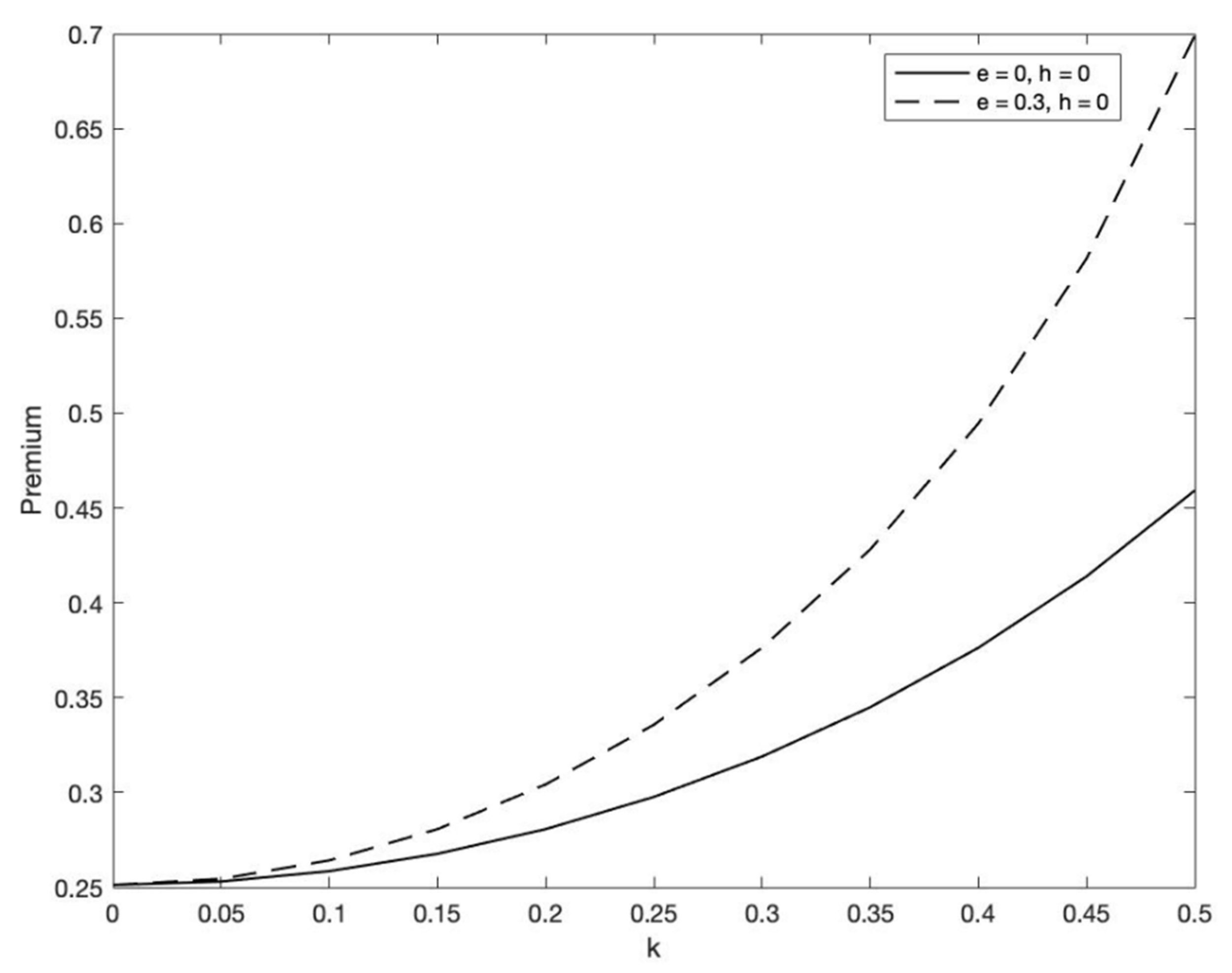
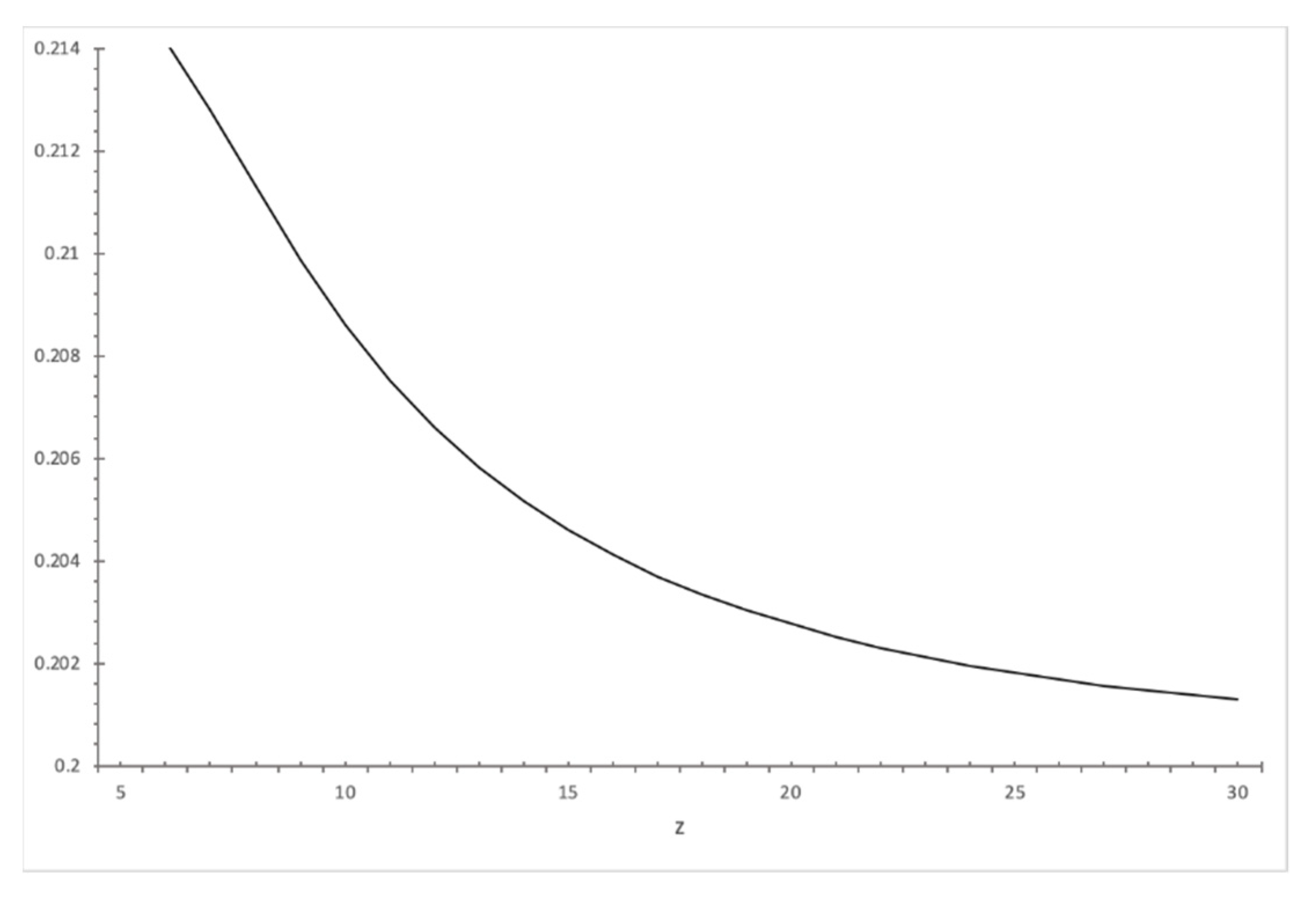
However, when external habits are present, the dynamics are more complex. This can be shown with a simple numerical example. Assume a CRRA utility function with coefficient of relative risk aversion . In Figure 1 and Figure 2 we have drawn the and respectively, when the background risk is distributed as . For a low background risk ( and no habits (), is uniformly decreasing (Figure 1), implying that the indirect utility function has a concave absolute risk tolerance.
But with the presence of habits, such as in the case of , can be decreasing or increasing (Figure 2), implying that the absolute risk tolerance might be concave or convex.
Proposition.
Suppose we have an economy with HARA preferences and habit formation, a level of risk aversion
, and a background risk that is small relative to wealth . Then the absolute risk tolerance of habit-forming agents might be concave or convex, implying that wealth inequality may increase or decrease the equity risk premium6.
Proof:
Assuming that and is distributed as , with and , then a second order Taylor approximation around would yield:
transforms as:
which can be rewritten as follows:
Due to the linearity of , the term is equal to 0. The term is expanded as:
where . Given that preferences are HARA, we have:
where . The term becomes:
The interaction of habits with risk aversion can reduce or increase . When habit formation is absent, term reduces into form (16) below, denoted as .
with .
Comparing and we find that if then > . This is always true for , regardless of the habit strength . Then , where is the reduced form of without habits (see Note 3). This in turn implies that , where is the absolute risk tolerance of an agent with habits and denotes the absolute risk tolerance of an agent without habits. Given that is concave, this should be sufficient to explain that can be concave ( or convex (. □
2.4. Asset Pricing
In an economy with background risk, the equilibrium price of an asset is , where is the asset’s payoff. Risky assets and bonds have payoff vectors and , respectively.
The relative price of a risky asset with respect to bonds is evaluated as:
The risk-free asset provides one unit of consumption good at with probability . The price of the bond will be:
where is the gross risk-free rate, is the current level of income per capita and is the income per capita at the maturity of the gross risk-free rate.
Subsequently, the risk-free rate is equal to:
3. Calibration and Results
We also examine numerically the effect on the equity risk premium in an economy with external habits, endowment inequality and background risk. In order to be able to compare our calibration findings with Gollier’s (2001a) we explore an economy with similar characteristics. In period the consumption per capita is certain and equal to . In period , two states of the world exist, a recession indexed by 1 and a growth state which is indexed by 2. In state 1 the per capita consumption becomes with a probability of 61.8%. In state 2 the per capita consumption becomes with a probability of 38.2%. We also note that our qualitative results do not depend on the probability of a recession, and they do not depend on the particular values of the growth rate of the per capita consumption in each state either. The mean and the variance of the growth rate of this economy are the same as those of the U.S. economy for the period 1889–1978 (See Table 1 data).
In terms of the wealth distribution of the economy, we run a simulation of two equally weighted classes, poor and rich. The poor are endowed with a share of of the GDP per capita in each state, and the rich are endowed with the rest . Parameter is the coefficient of variation of the wealth distribution. Parameter measures the degree of relative risk aversion evaluated at consumption level and is set at , which is reasonable and consistent with the finance literature. Lastly, we introduce an uninsurable labor income risk , distributed as , i.e., a background risk will yield a 50-50 chance to win or lose . Parameter is the standard deviation of the growth of labor income.
The introduction of external habits has a complex effect on the concavity of the absolute risk tolerance. We find that with low background risk ( wealth inequality may increase or decrease the equity premium in an economy with external habits. Table 2 provides evidence for the ambiguity of results.
The first column of Table 2 refers to a non-habit economy () and confirms Gollier’s (2001a) results. The next three columns refer to a habit economy with weak (), moderate () and strong habits (.5), respectively. In all cases, the level of income uncertainty is low and kept fixed at . We observe that, for weak habit strength, wealth inequality () will increase the equity risk premium in an incomplete market setting. However, for stronger habits ( equal to or ), wealth inequality will decrease the equity risk premium. This result extends Gollier’s (2001a) findings on the relationship between inequality, income uncertainty and the risk premium. Wealth inequality can decrease the equity risk premium even with a low level of background risk when investors exhibit exogenously habit-forming preferences. However, as we observe, the values for the premium continue to be low, given a low level of background risk.
Next, we examine the effect of habits on the equity risk premium as the level of income uncertainty rises. Figure 3, Figure 4, Figure 5 and Figure 6 show the equity risk premium as a function of the size of the uninsurable income risk. In the finance literature it has been shown that external habits will raise the equity risk premium in a conventional C-CAPM complete market model with CRRA preferences. In these models, wealth inequality has no effect on asset pricing. Our simulations suggest that in an incomplete market model, where wealth inequality matters, external habits will also increase the equity risk premium.
Figure 3 compares non-habits with habits in an egalitarian economy with background risk, while Figure 4 compares a non-habit with a habit case in an unequal economy (). We observe that external habits increase the equity risk premium in both egalitarian and unequal economies. The increase of the premium is substantially higher as the background risk increases. With absence of background risk, the increase in premium can be characterized as marginal. It seems that background risk amplifies the effect of habits.
Another observation that we make is that, when the level of income uncertainty is high, wealth inequality will decrease the equity risk premium even after the introduction of external habits. In the non-habit economy with , wealth inequality produces a premium below 0.45% (Figure 4), while in the egalitarian case, the premium is above 0.45% (Figure 3). With habits the results for the equity premium diverge substantially. Specifically, for habit strength , the risk premium is slightly above 0.6% in the unequal economy (Figure 4), while in the egalitarian economy is as high as 0.7% (Figure 3).
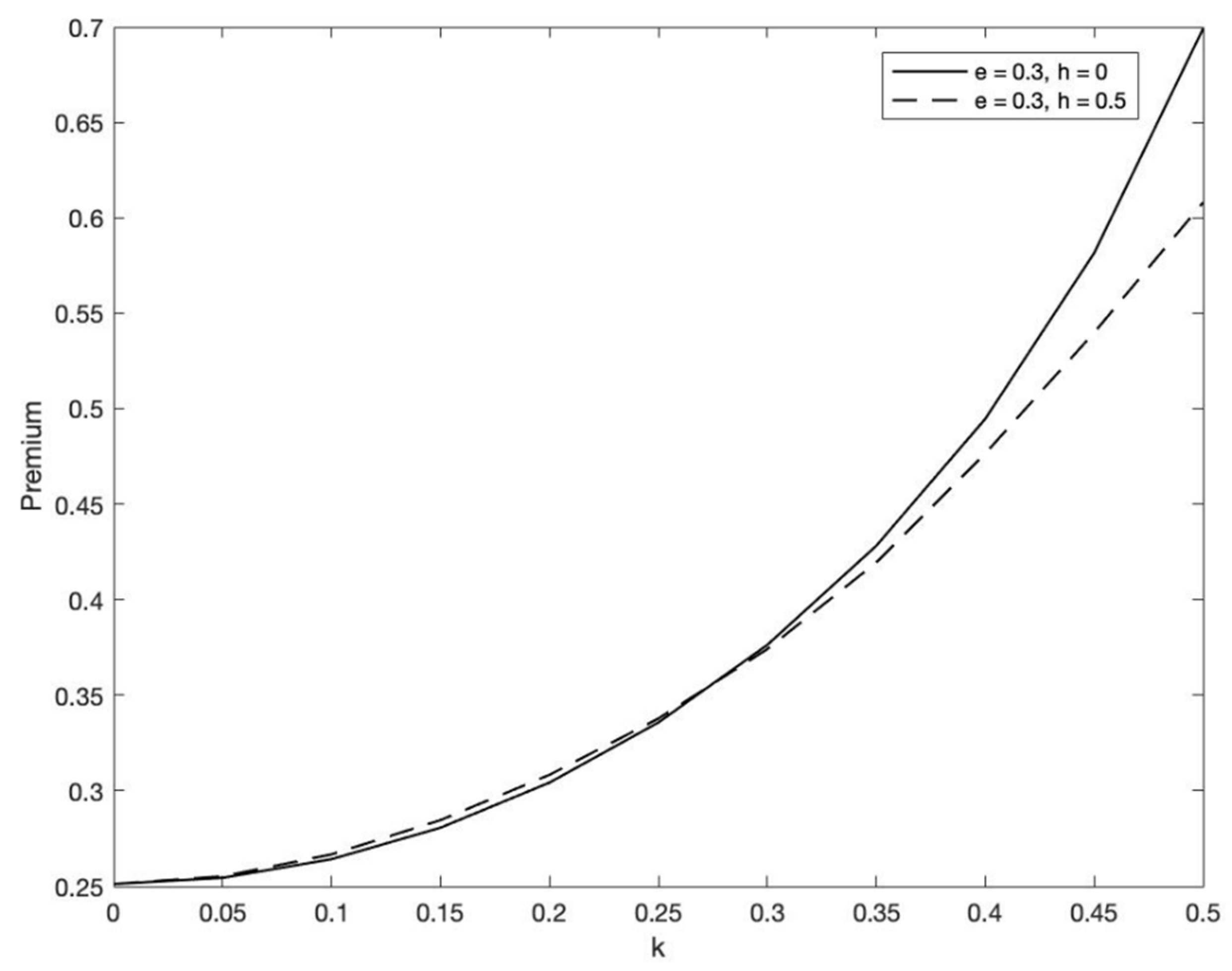
Figure 5 and Figure 6 extend further our analysis. Figure 5 replicates Gollier’s (2001a) findings and compares an egalitarian with an unequal economy () where agents exhibit non-habit preferences (), while Figure 6 compares an egalitarian with an unequal economy () and refers to the habit scenario ().
We observe that for a larger income uncertainty () and absence of habits (Figure 5), wealth inequality will decrease the equity risk premium. However, in the scenario of the habit economy (Figure 6), wealth inequality will decrease the equity risk premium even when a low background risk is present (.
It seems that the effects that habits have in our model economy are magnified when wealth inequality and a high level of income uncertainty are present. The highest equity premium is generated in an egalitarian economy with habits and large background risk. It becomes evident that even after the introduction of external habits, wealth inequality continues to have a small effect in adjusting the equity premium to its empirically observed levels. We leave potential empirical tests of the above results for future research.
4. Conclusions
The objective of this study is to examine the relationship between asset prices, wealth inequality, external habit formation and market incompleteness in the form of background risk. Wealth inequality is established with a mean preserving transfer of endowment. When consumers have HARA preferences without habits and face no uninsurable risk, the distribution of wealth has no effect on the equity premium and on the risk-free rate. We inquire about whether taking into account the unequal distribution of wealth in an economy with background risk may contribute to the equity premium puzzle, when the preferences of the agents are habit forming.
Stronger external habits can substantially increase the equity risk premium. The highest equity premium is generated in an egalitarian economy with external habits and large background risk. Furthermore, we show that in a habit economy it is ambiguous whether wealth inequality will increase or decrease the equity risk premium when a low background risk is present. Specifically, we extend Gollier’s (2001a) findings and show that wealth inequality may decrease the equity risk premium even when an economy has a low level of income uncertainty, as long as external habits are present. However, wealth inequality continues to have a small effect on asset pricing, even after the introduction of external habits.
An explanation for the marginal effect of wealth inequality on asset prices can be attributed to the curvature of the conventional HARA utility function and its variations. Specifications of the C-CAPM where the stochastic discount factor is based on higher order Taylor expansions of arbitrary smooth utility functions, such as the one described by Harvey and Siddique (2000), might be able to exhibit essentially arbitrary amounts of curvature. Although follow-up work such as Post et al. (2008) and Poti and Wang (2010) suggested that, under appropriate restrictions, higher moment C-CAPM type of models might be more limited than what was initially expected, these models do not account for the presence of background risk and wealth inequality. This is clearly a rational and possible application of our work. The evaluation of the effect of background risk and wealth inequality in this case is left to future research.
Author Contributions
All authors have equally contributed for the preparation of this paper (Conceptualization, Methodology, Data, Software, Validation, Formal analysis, Writing—original draft, Writing—review & editing, Project administration). All authors have read and agreed to the published version of the manuscript.
Funding
This research received no external funding.
Acknowledgments
We wish to thank the Editor and two anonymous referees for their comments and helpful suggestions that helped us improving the quality of our paper. We are especially grateful to a referee for suggesting a rationale and application of our work. Christos I. Giannikos acknowledges summer research support from the Bert W. Wasserman Department of Economics and Finance, Zicklin School of Business, Baruch College, CUNY. Georgios Koimisis acknowledges summer research support from the O’Malley School of Business, Manhattan College. The usual caveat applies.
Conflicts of Interest
The authors declare no conflict of interest.
Appendix A. Risk Free Rate
To analyze the impact of wealth inequality and external habits on the risk-free rate, a discussion on the concept of prudence is required. The global effect of wealth inequality is decomposed into a consumption smoothing effect and a precautionary savings effect, with the latter being the relevant for our analysis. The absolute risk prudence measures the intensity of precautionary savings (Kimball 1990) and equals .
Gollier (2001a) proved that, when the risk-free rate is smaller (larger) than the rate of pure preference for the present in the egalitarian economy, wealth inequality decreases the risk-free rate if the inverse of absolute prudence is concave, and the absolute risk tolerance is concave (convex). The analysis for the absolute risk tolerance is in Section 2 of this paper.
Our economy is characterized by an element of market incompleteness in the form of a background risk and from preferences formed by the utility function . We denote the absolute imprudence of without habits as and the absolute imprudence of with habits as . The of equals:
when evaluated at . Differentiating with respect to yields:
and
where
Gollier (2001a) showed that for low background risk the absolute imprudence of investors will be concave and therefore wealth inequality will decrease the risk-free rate, as long as the risk-free rate is less than . In an economy with low background risk but with absence of habit formation, would be negative and non-negative, reducing our case to Gollier’s (2001a).
However, as in the case of absolute risk tolerance, when external habits are present the dynamics are more complex. This can be shown with the following numerical example. Assume a CRRA utility function (as the one in Section 2.3) with coefficient of relative risk aversion .
In Figure A1 and Figure A2 we have drawn the , and respectively, when the background risk is distributed as . For a low background risk ( and no habits (), is uniformly decreasing (Figure A1), implying that the indirect utility function has a concave absolute imprudence.
However, when habits are present (Figure A2), such as in the case of , the absolute imprudence might be concave or convex.
As in the case of the absolute risk tolerance, we work similarly the relationships (11)–(16) for the absolute risk imprudence , except for replacing with . The results imply that , where is the absolute risk imprudence of an agent with habits and denotes the absolute risk imprudence of an agent without habits. Given that is concave, this should be sufficient to explain that can be concave ( or convex (. Then if in the egalitarian economy, wealth inequality might decrease or increase the risk-free rate.
| 1 | |
| 2 | This mechanism allows the departure from an egalitarian wealth distribution. |
| 3 | Giannikos and Koimisis (2021) explore a similar model specification, but in a market with full consumption insurance and a type of utility function that allows for flexible risk tolerance. |
| 4 | |
| 5 | |
| 6 | This proposition can be extended for the risk-free rate (See Appendix A for analysis). |
References
- Abel, Andrew B. 1990. Asset Prices Under Habit Formation and Catching Up with the Joneses. American Economic Review 80: 38–42. [Google Scholar]
- Bodie, Zvi, Robert C. Merton, and William F. Samuelson. 1992. Labor Supply Flexibility and Portfolio Choice in a life Cycle Model. Journal of Economic Dynamics and Control 16: 427–49. [Google Scholar] [CrossRef] [Green Version]
- Campbell, John Y., and John H. Cochrane. 1999. By Force of Habit: A Consumption-Based Explanation of Aggregate Stock Market Behavior. Journal of Political Economy 107: 205–51. [Google Scholar] [CrossRef]
- Cocco, João F. 2005. Portfolio Choice in the Presence of Housing. The Review of Financial Studies 18: 535–67. [Google Scholar] [CrossRef]
- Cocco, João F., Fransisco Gomes, and Pascal J. Manehout. 2005. Consumption and Portfolio Choice over the Life-Cycle. Review of Financial Studies 18: 491–533. [Google Scholar] [CrossRef]
- Constantinides, George M. 1990. Habit Formation: A Resolution of the Equity Premium Puzzle. Journal of Political Economy 98: 519–43. [Google Scholar] [CrossRef]
- Constantinides, George M., and Darrell Duffie. 1996. Asset pricing with heterogeneous consumers. Journal of Political Economy 104: 219–40. [Google Scholar] [CrossRef]
- Eeckhoudt, Louis, Christian Gollier, and Harris Schlesinger. 1996. Changes in Background Risk and Risk Taking Behavior. Econometrica 64: 683–89. [Google Scholar] [CrossRef] [Green Version]
- Fagereng, Andreas, Luigi Guiso, and Luigi Pistaferri. 2018. Portfolio Choices, Firm Shocks, and Uninsurable Wage Risk. Review of Economic Studies 85: 437–74. [Google Scholar]
- Favilukis, Jack. 2013. Wealth Inequality, Stock Market Participation, and the Equity Premium. Journal of Financial Economics 107: 740–59. [Google Scholar] [CrossRef] [Green Version]
- Ferson, Wayne E., and George M. Constantinides. 1991. Habit Persistence and Durability in aggregate consumption. Journal of Financial Economics 29: 199–240. [Google Scholar] [CrossRef]
- Flavin, Marjorie, and Takashi Yamashita. 2002. Owner-Occupied Housing and the Composition of the Household Portfolio. American Economic Review 92: 345–62. [Google Scholar] [CrossRef]
- Gârleanu, Nicolae, and Stavros Panageas. 2015. Young, Old, Conservative, and Bold: The Implications of Heterogeneity and Finite Lives for Asset Pricing. Journal of Political Economy 123: 670–85. [Google Scholar] [CrossRef]
- Giannikos, Christos I., and Georgios Koimisis. 2021. Habits, Wealth and Equity Risk Premium. Finance Research Letters 38: 101518. [Google Scholar] [CrossRef]
- Gollier, Christian. 2001a. Wealth Inequality and Asset Pricing. Review of Economic Studies 68: 181–203. [Google Scholar] [CrossRef]
- Gollier, Christian. 2001b. The Economics of Risk and Time. Cambridge: MIT Press. [Google Scholar]
- Gollier, Christian. 2021. Habit Persistence reduces Risk Aversion. The Geneva Papers on Risk and Insurance—Issues and Practice 46: 214–23. [Google Scholar] [CrossRef]
- Gollier, Christian, and John W. Pratt. 1996. Risk vulnerability and the tempering effect of background risk. Econometrica 64: 1109–23. [Google Scholar] [CrossRef]
- Harvey, Campbell R., and Akhtar Siddique. 2000. Conditional skewness in asset pricing tests. Journal of Finance 55: 1263–95. [Google Scholar] [CrossRef]
- Heaton, John, and Deborah Lucas. 2000a. Portfolio Choice in the Presence of Background Risk. Economic Journal 110: 1–26. [Google Scholar] [CrossRef]
- Heaton, John, and Deborah Lucas. 2000b. Asset Pricing and Portfolio Choice: The Importance of Entrepreneurial Risk. Journal of Finance 55: 1163–98. [Google Scholar] [CrossRef]
- Kimball, Miles S. 1990. Precautionary Saving in the Small and in the Large. Econometrica 58: 53–73. [Google Scholar] [CrossRef] [Green Version]
- Kimball, Miles S. 1993. Standard Risk Aversion. Econometrica 61: 589–611. [Google Scholar] [CrossRef]
- Krusell, Per, and Anthony A. Smith. 1997. Income and Wealth Heterogeneity, Portfolio Choice, and Equilibrium Asset Returns. Macroeconomic Dynamics 1: 387–422. [Google Scholar] [CrossRef] [Green Version]
- Mehra, Rajnish, and Edward C. Prescott. 1985. The Equity Premium: A Puzzle. Journal of Monetary Economics 15: 145–61. [Google Scholar] [CrossRef]
- Post, Thierry, Pim van Vliet, and Haim Levy. 2008. Risk aversion and skewness preference. Journal of Banking and Finance 32: 1178–87. [Google Scholar] [CrossRef]
- Poti, Valerio, and Dengli Wang. 2010. The coskewness puzzle. Journal of Banking and Finance 34: 1827–38. [Google Scholar] [CrossRef]
- Pratt, John W., and Richard J. Zeckhauser. 1987. Proper Risk Aversion. Econometrica 55: 143–54. [Google Scholar] [CrossRef]
- Semenov, Andrei. 2017. Background risk in consumption and the equity risk premium. Review of Quantitative Finance and Accounting 48: 407–39. [Google Scholar] [CrossRef]
- Sundaresan, Suresh M. 1989. Intertemporally dependent preferences and the volatility of consumption and wealth. The Review of Financial Studies 2: 73–89. [Google Scholar] [CrossRef] [Green Version]
- Toda, Alexis A., and Kieran J. Walsh. 2020. The Equity Premium and the One Percent. The Review of Financial Studies 33: 3583–623. [Google Scholar] [CrossRef]
- Viceira, Luis M. 2001. Optimal Portfolio Choice for Long-Horizon Investors with Nontradable Labor Income. Journal of Finance 56: 433–70. [Google Scholar] [CrossRef]
- Weil, Philippe. 1989. The Equity Premium Puzzle and the Risk Free Rate Puzzle. Journal of Monetary Economics 24: 401–21. [Google Scholar] [CrossRef]
- Yao, Rui, and Harold H. Zhang. 2005. Optimal Consumption and Portfolio Choices with Risky Housing and Borrowing Constraints. Review of Financial Studies 18: 197–239. [Google Scholar] [CrossRef]
Figure 1.
when and .

Figure 2.
when and .

Figure 3.
The equity premium (in %) as a function of the background risk. The solid (dashed) line represents the non-habit (habit) egalitarian economy.
Figure 3.
The equity premium (in %) as a function of the background risk. The solid (dashed) line represents the non-habit (habit) egalitarian economy.

Figure 4.
The equity premium (in %) as a function of the background risk. The solid (dashed) line represents the non-habit (habit) unequal economy.
Figure 4.
The equity premium (in %) as a function of the background risk. The solid (dashed) line represents the non-habit (habit) unequal economy.

Figure 5.
The equity premium (in %) as a function of the background risk. The solid (dashed) line represents the non-habit egalitarian (unequal) economy.
Figure 5.
The equity premium (in %) as a function of the background risk. The solid (dashed) line represents the non-habit egalitarian (unequal) economy.

Figure 6.
The equity premium (in %) as a function of the background risk. The solid (dashed) line represents the habit egalitarian (unequal) economy.
Figure 6.
The equity premium (in %) as a function of the background risk. The solid (dashed) line represents the habit egalitarian (unequal) economy.

Figure A1.
when and .

Figure A2.
when and .


Table 1.
Summary Statistics, United States Annual Data, 1889–1978.
| Estimates | |
|---|---|
| 1.82 (3.61) | |
| 0.77 (5.92) | |
| 6.98 (16.54) | |
| 6.21 (16.76) |
Note: Sample mean and sample standard deviation (in parentheses) figures for real consumption growth , the real risk-free interest rate , real return on equity and the equity risk premium . All values are in percentages. Source: Mehra and Prescott (1985).
Table 2.
Equity Risk Premium (in %).
| 0.0 | 0.1 | 0.3 | 0.5 | |
|---|---|---|---|---|
| 0.0 | 0.3038 | 0.3153 | 0.3491 | 0.4687 |
| 0.3 | 0.3059 | 0.3174 | 0.3500 | 0.4632 |
| 0.5 | 0.3089 | 0.3198 | 0.3495 | 0.4414 |
Note: Calibration results for the equity risk premium , in an economy with external habits and low background risk (.
Publisher’s Note: MDPI stays neutral with regard to jurisdictional claims in published maps and institutional affiliations. |
© 2021 by the authors. Licensee MDPI, Basel, Switzerland. This article is an open access article distributed under the terms and conditions of the Creative Commons Attribution (CC BY) license (https://creativecommons.org/licenses/by/4.0/).
Share and Cite
MDPI and ACS Style
Giannikos, C.I.; Koimisis, G. Equity Premium with Habits, Wealth Inequality and Background Risk. J. Risk Financial Manag. 2021, 14, 321. https://0-doi-org.brum.beds.ac.uk/10.3390/jrfm14070321
AMA Style
Giannikos CI, Koimisis G. Equity Premium with Habits, Wealth Inequality and Background Risk. Journal of Risk and Financial Management. 2021; 14(7):321. https://0-doi-org.brum.beds.ac.uk/10.3390/jrfm14070321
Chicago/Turabian StyleGiannikos, Christos I., and Georgios Koimisis. 2021. "Equity Premium with Habits, Wealth Inequality and Background Risk" Journal of Risk and Financial Management 14, no. 7: 321. https://0-doi-org.brum.beds.ac.uk/10.3390/jrfm14070321