
Bankruptcy Prediction Using Machine Learning Techniques

1
College of Business Administration, Lamar University, Beaumont, TX 77705, USA
2
Department of Mathematics & Natural Science, College of Arts & Sciences, Gulf University for Science & Technology, Mishref 32093, Kuwait
3
Warocqué School of Business and Economics, University of Mons, 7000 Mons, Belgium
*
Author to whom correspondence should be addressed.
J. Risk Financial Manag. 2022, 15(1), 35; https://0-doi-org.brum.beds.ac.uk/10.3390/jrfm15010035
Submission received: 9 July 2021
/
Revised: 10 November 2021
/
Accepted: 12 November 2021
/
Published: 13 January 2022
(This article belongs to the Special Issue Asset Allocation)
Abstract
:In this study, we apply several advanced machine learning techniques including extreme gradient boosting (XGBoost), support vector machine (SVM), and a deep neural network to predict bankruptcy using easily obtainable financial data of 3728 Belgian Small and Medium Enterprises (SME’s) during the period 2002–2012. Using the above-mentioned machine learning techniques, we predict bankruptcies with a global accuracy of 82–83% using only three easily obtainable financial ratios: the return on assets, the current ratio, and the solvency ratio. While the prediction accuracy is similar to several previous models in the literature, our model is very simple to implement and represents an accurate and user-friendly tool to discriminate between bankrupt and non-bankrupt firms.
1. Introduction
Bankruptcy detection is a major topic in finance. Indeed, for obvious reasons, many actors such as shareholders, managers or banks are interested in the likelihood of bankruptcy of firms. Consequently, many studies have been carried out on the topic of bankruptcy prediction. In the late 1960s, Beaver (1966) introduced a univariate analysis, providing the first statistical justification for the ability of financial ratios to account for default. Then, Altman (1968) developed the Z-score model by using five financial ratios to predict the bankruptcy of U.S. firms. In his paper, Altman employed multiple discriminant analysis (MDA) techniques to determine the probability of bankruptcy on a sample of firms. Altman’s Z-Score model has been a popular technique and widely used by auditors, accountants, courts, banks, and other creditors. The MDA technique assumes that variables follow a normal distribution, and this methodology was later adopted by many other researchers (Deakin 1972; Edmister 1972; Altman et al. 1977; Laitinen 1991; Grice and Ingram 2001). The hypothesis of multinormality of variables is then questioned in favor of the hypothesis according to which the explanatory variables have different distributions. Consequently, the logit (Ohlson 1980) and probit (Zmijewski 1984) models were then frequently used in the prediction of the failure. The second stage of the story began in the 1990s with artificial intelligence algorithms, specifically in the machine learning branch such as neural networks (Lennox 1999) or the genetic algorithm (Shin and Lee 2002). They produced convincing results in terms of forecasting without requiring any statistical restriction. Indeed, Barboza et al. (2017) tested five machine learning models and compared their bankruptcy prediction power against traditional statistics techniques (discriminant analysis and logistic regression) using North American firms’ data from 1985 to 2013. Their study found substantial improvement in bankruptcy prediction accuracy using machine learning techniques compared to traditional methods. This conclusion is also reached by (Adnan and Dar 2006) through their extensive literature review. Ongoing, in the 21st century, new types of learning machines such as extreme gradient boosting (XGBoost), support vector machine, random forest or deep neural network were developed and often provided better accuracy than statistical techniques. Shi and Li (2019) literature review reports that logit and neural network models are the most frequently used and studied models in the area of bankruptcy prediction. Mai et al. (2018) compared traditional learning machine models with convolutional neural networks on a large database of US public companies and report that simpler models are more effective, while Hosaka’s study (Hosaka 2019), based on a smaller sample of delisted Japanese companies, reports that the use of convolutional neural networks allows to reach better predictions. So far, no consensus regarding the use of convolutional neural networks exists.
In addition to the choice of the model, bankruptcy prediction accuracy depends on the financial ratios that are chosen to run the model. To this end, statisticians have developed methods such as principal components analysis (Zavgren 1985; Wang 2004; Tang and Chi 2005; Pompe and Bilderbeek 2005) or LASSO1 technique (Meir et al. 2008; Tian et al. 2015) for selecting subsets of variables from an initial list of explanatory variables to identify the most relevant predictor variables (Fan and Li 2001). These lists may include 50 ratios (du Jardin 2015) that are built using detailed information from the balance sheet and the income statement. Out of these lists, 5 to 10 ratios are generally retained to run the model. Du Jardin’s study (du Jardin 2006) reports several variable selection methods. Even though most studies use annual data one year prior to bankruptcy, Baldwin and Glezen (1992) resorted to quarterly data to feed their model and Reznakova and Karas (2014) calculate averaged ratios involving several years before bankruptcy. Some studies include nonfinancial variables (in addition to financial ratios) into bankruptcy prediction models. These variables may refer to market valuation (Campbell et al. 2008; Tian et al. 2015), corporate governance (Ciampi 2015), relational (Tobback et al. 2017) or textual data (Mai et al. 2018). Other specificities may exist. Pompe and Bilderbeek (2005) investigated the influence of the model accuracy in a period of economic decline. Bankruptcy prediction models can be related to SME’s (Brédart and Cultrera 2016) or to listed firms (Sfakianakis 2012). Nevertheless, the availability of this detailed information for some firms may be questioned.
Similar to many other western countries, Belgium has accounted for many bankruptcies in the recent past. Brédart’s (2014) study utilized Belgian bankruptcies data to predict bankruptcies using the neural networks method and reached good prediction accuracy-above 80%. In this paper, we replicate Brédart’s study using a simple neural network with one layer, and four cutting-edge machine learning techniques: a deep feed-forward network with six hidden layers, Random Forests, Support Vector Machine with radial basis function kernel and Extreme Gradient Boosting (XGBoost) to compare their performances. Even though Brédart used only three variables in his model, the prediction accuracy was fairly good. In our study, we used the same financial ratios that were considered by Brédart as they have a good bankruptcy prediction rate. Our objective in this study is to utilize sophisticated machine learning techniques to see if these techniques have better predictability using the Brédart’s data from Belgium compared to his model involving the neural networks method.
Our results report prediction accuracy rates of more than 80 percent, using only three easily obtainable financial ratios: the return on assets, the current ratio, and the solvency ratio. Even though, Barboza et al.’s (2017) study had significantly higher prediction accuracy using machine learning techniques compared to the traditional methods, our study did not show any improvement in prediction from the machine learning techniques compared to the shallow neural network method with a single hidden layer. All the four methods gave the same kind of results of about 81% prediction accuracy. The graphical plots of the data show a significant overlap between the different features of the bankrupt and solvent firms’ data. This leads to a limitation of advanced models to carry out better predictions. Nevertheless, the ease of collecting the information feeding our models makes them very attractive for decision makers such as bankers. Our study contributes to the academic literature about bankruptcy prediction because it shows that simple models using easily obtainable and common information can be reliable and help to make adequate decisions.
2. Data and Methodology
2.1. Data
In this study, we used the same Belgian firm’s dataset previously used by Brédart (Brédart 2014). This dataset consists of a sample of 3728 Belgian firms that were declared bankrupt between 2002 and 2012 to predict bankruptcy utilizing the new bankruptcy prediction techniques. We used the same three financial ratios that were considered by this author as they were simple, easily available and provided good classification rates.
2.2. Methodology
To predict bankruptcy, we utilized several of the most advanced machine learning techniques, including, a deep neural network, support vector machine (SVM) and extreme gradient boosted tree method (XGBoost). These techniques are described hereafter.
2.2.1. Deep Feedforward Neural Networks
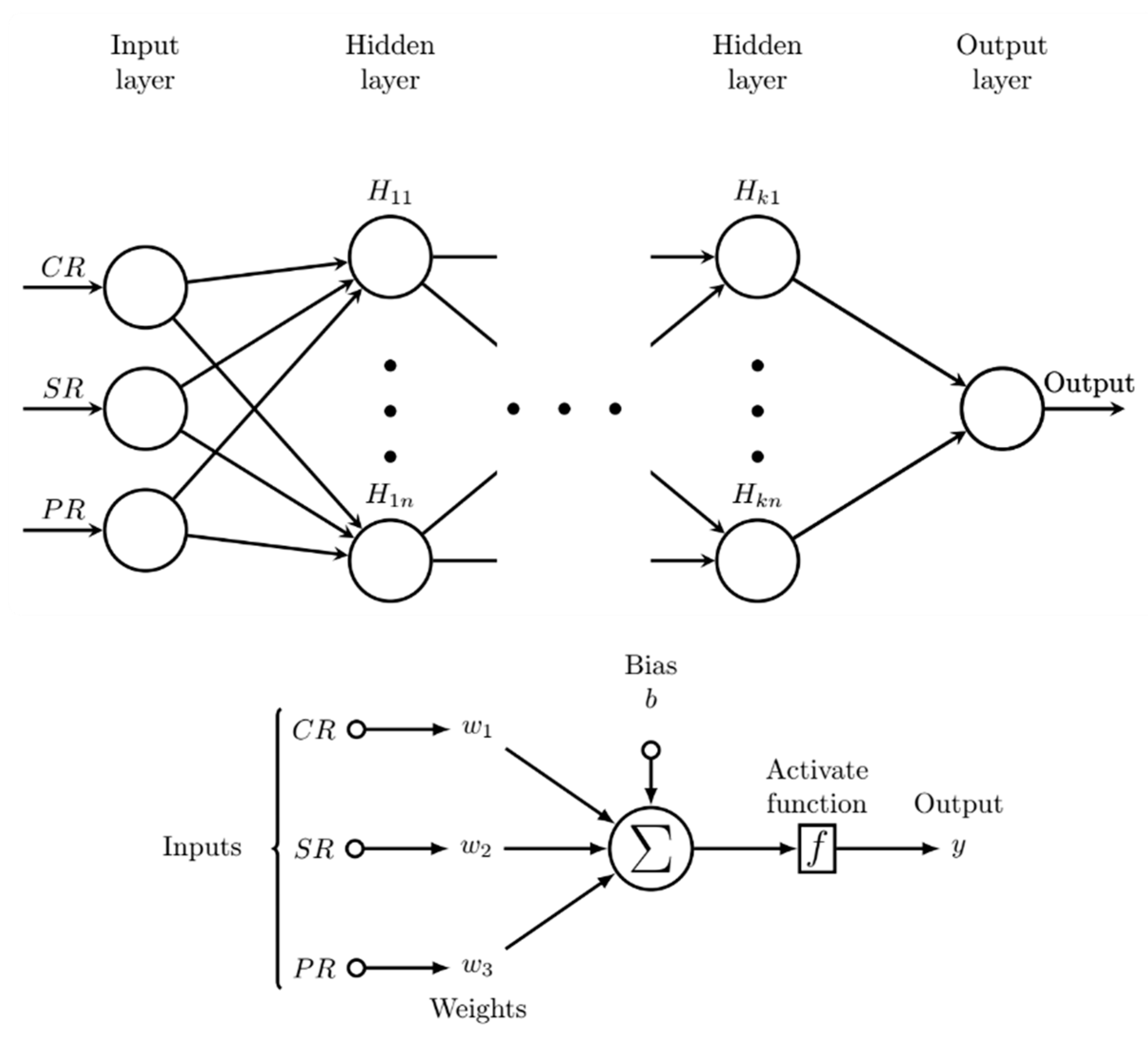
Deep feedforward artificial neural networks are advanced types of supervised machine learning methods which learn patterns in the input data through compositions of mathematical functions in order to map input data to corresponding outputs (Goodfellow et al. 2016). Deep feedforward networks are capable of performing both regression and classification tasks. As shown in Figure 1, a typical feedforward network consists of three types of layers: an input layer, which receives the data, an output layer, which represents the network output, and a number of hidden layers, which perform the task of mapping the input features to the network output. Each hidden layer consists of a set of non-interacting neurons, which processes the data in a parallel manner. The width of the network is determined by the number of neurons in the hidden layers, whereas the depth of the networks is a measure of the number of its hidden layers. A shallow neural network has up to several hidden layers, whereas usually a deep network has a larger number of hidden layers. Figure 1 shows a schematic diagram of a fully connected feed-forward network. The upper figure shows the general structure of the network, whereas the lower figure shows the schematic diagram of the artificial neuron.
A feedforward network is said to be fully connected if each neuron in a specific layer receives the outputs of all the neurons in the previous layers. As illustrated in Figure 1 (lower panel), the neurons perform a two-step mathematical operation: First each performs a scalar product between its input vector and its local weight vector, and the result is shifted by the addition of a scalar bias. In the second step, the result is transformed through the activation function of the neural.
The training stage of the network starts with the data being individually propagated forward through the network to generate the corresponding error signal
due to the discrepancy between the network’s predicted output f(xi) and the ground truth yi. Next, a backward propagation step is initiated where the “gradient decent” optimization method is applied to adjust the weights in order to reduce the network output error. In “online learning”, the two-step learning process is applied to each datum individually, whereas in “batch learning”, the error due to batch of data (m input data) is propagated through the network before their collective error is computed as
and the weights adjusted (Goodfellow et al. 2016).
The training data is usually divided into three batches, named appropriately as “training set”, “development set”, and “testing set”. The training set accounts for the largest of the three sets (60–70%) and is used to optimize the network accuracy by repeatedly using it until the desired accuracy is reached. The development portion of the data is then used to test the accuracy of the network with previously unseen data. This step is crucial to diagnose over-fitting and related issues. Any significant discrepancy between the network’s accuracy for the training and development will lead to repeating the training process, possibly adjusting the network hyperparameters (batch size, learning rate, etc.) or structure (number of layers, etc.) or introducing a regularization scheme. After the network reaches the desired level with the development set, the testing set is used to determine the ultimate accuracy of the network. There are several popular packages that offer implementations of deep neural networks, most prominent of which are Python-based Google’s Tensflow and Facebook’s PyTorch. These packages offer multiple tools for implementation and regularization of neural networks, such as drop-out and Lp norm methods. In this study we used Tensorflow implementation of deep feedforward network to predict bankruptcy/solvency ratios.
2.2.2. Support Vector Machine (SVMs)
Support vector machines (SVMs) are powerful supervised machine learning methods that are used mainly for classification. They are a class of optimal margin classifiers that find a boundary hypersurface (or plane) with maximal margin between data clusters belonging to different classes (Boser et al. 1992; Cortes and Vapnik 1995). SVMs have high classification efficiency for high-dimensional data, even in cases where different classes overlap significantly. Mathematically, the method finds a d-dimensional hyperplane satisfying the equation:
for the d-dimensional data point xi corresponding to output yi, where wj is the corresponding is jth component of the weight vector and ζ is a soft margin slack variable used to adjust the boundary between classes in such a way as to minimize the classification error while allowing misclassification of overlapping data points. If the data is linearly separable, the method generalizes perfectly to previously unseen data (Abe 2005). If there is no linear separability, then it is mapped into a higher-dimensional scalar product space through a set of functional transformations where the dot products in the above inequality are replaced by products of functions of the data. The above inequality takes the new form:
for , where are functions that cast the data in to high-dimensional feature space that eliminates or reduces the degree of overlap between the different classes in an attempt to improve the generalization accuracy of the model.
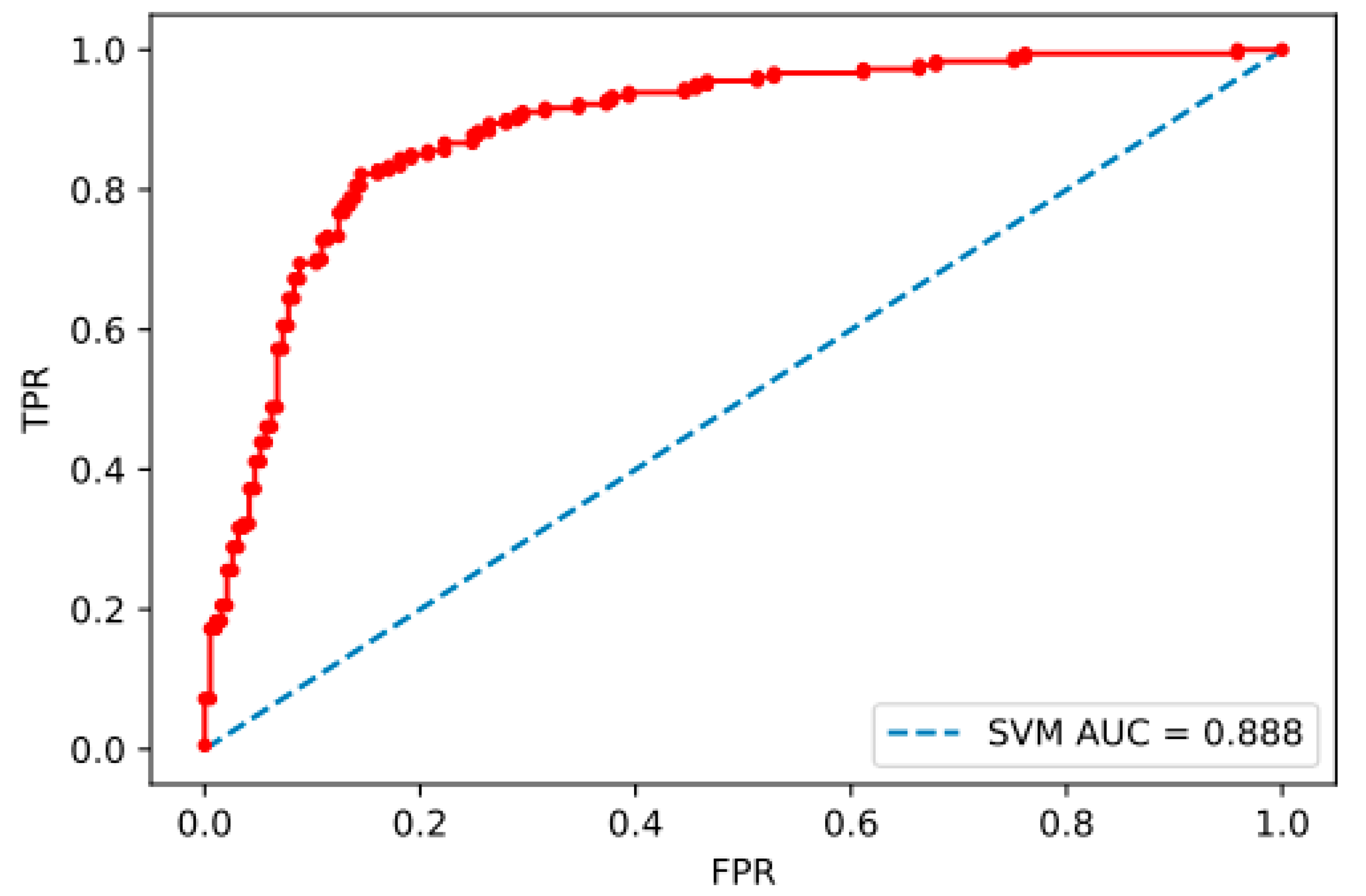
In practice, to find the optimal decision boundary between the data classes, algorithms implementing the SVM model utilize a two-step iterative optimization process. In the first step, the data is cast into a high-dimensional space to find a decision hyper-plane. In the second step, the distance between the resulting hyperplane and closest data points is tweaked in order to maximize the margin between the decision boundary and the nearest data points. The power of the of the SVM classifier lies in that it always finds a decision boundary, especially when there is significant overlap between the different data classes. After it finds such optimal boundary, the SVM model is ready to classify new data points according to which side of the decision boundary their coordinates lie. The SVM algorithm is implemented in various programming languages, including Python. The Python implementation of the SVM is included in the open-source machine learning package Scikit-Learn. The ROC curve of SVM model is shown in Figure 2.
2.2.3. Extreme Gradient Boosting
Boosting is a powerful, ensemble-based learning method that combines a set of easily learnable, weak classifiers into a much powerful classifier (Schapire 1990, 1999; Kearns and Valiant 1989). Extreme gradient boosting (XGBoost) is a variant of gradient boosting methods with superior performance that uses a more regularized model formalization to control overfitting (Chen and Guestrin 2016). Alongside deep learning, XGBoost is one of the most successful methods for large scale data classification and is the method of choice for many winning entries in Kaggle machine learning competitions. XGBoost is implemented in many programming languages, including Python as part of the Scikit-Learn package.
3. Results
Table 1 shows the correlations between variables that are used in the models to predict bankruptcy of Belgian firms. All the correlation coefficients are relatively small. The accuracy of the model for predicting the categories of new inputs as bankrupt or otherwise for the different classification algorithms is limited to around 81–82% range. The limitation in the accuracy is due to a significant overlap between the two classes as shown in Figure 3.
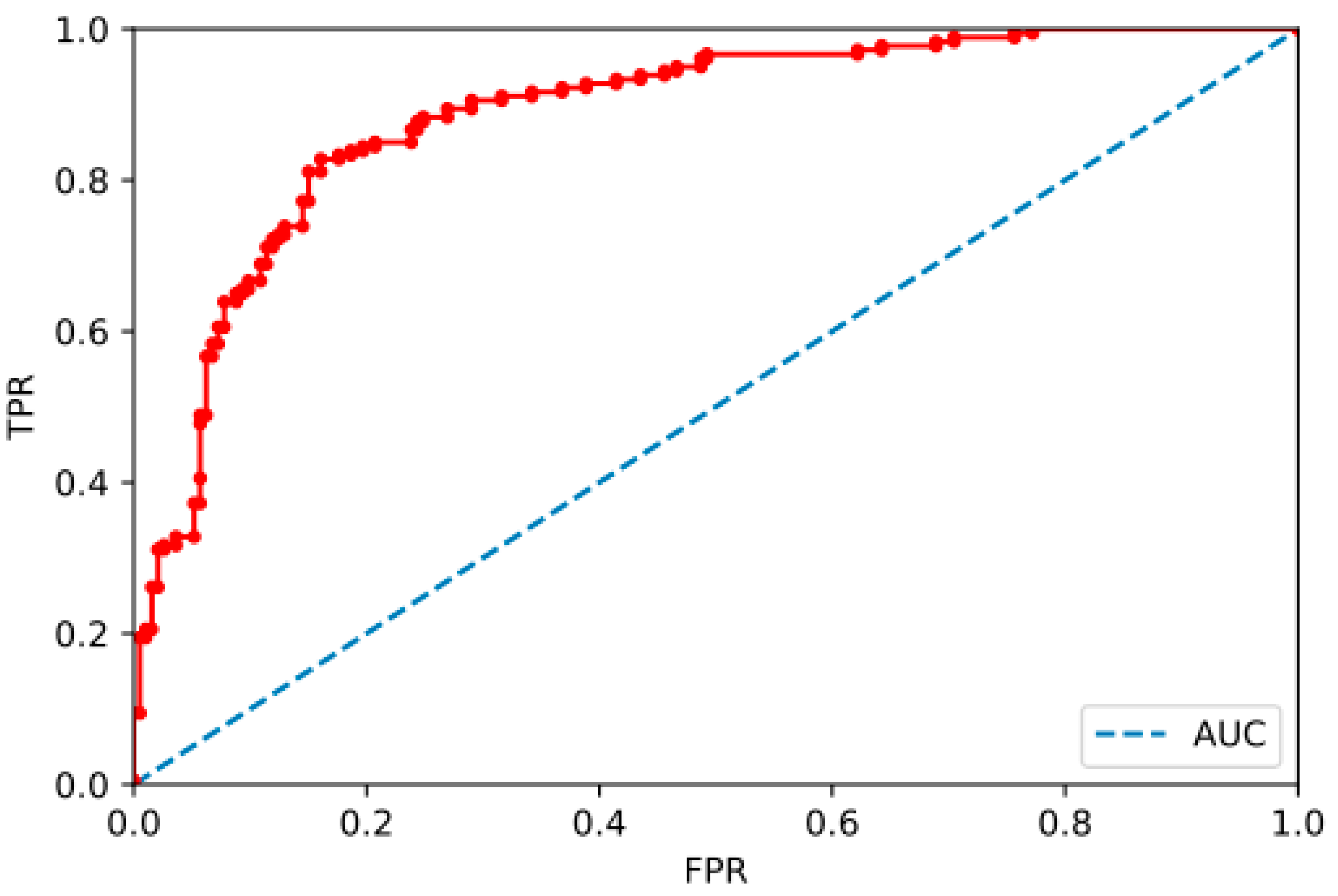
The Receiver Operating Characteristics (ROC) curve is plotted with true positive rate (TPR) against the false positive rate (FPR) using the feedforward neural networks model as shown in Figure 4. A higher y-axis in this plot indicates a higher number of true positives relative to false negatives. It represents goodness of the model in predicting the positive class when the actual outcome is positive. A better prediction performance can be expected if the curve is closer to the top-left corner of the plot. The area below the ROC curve is called the Area Under the Curve (AUC), which is the probability that a randomly chosen bankruptcy is higher than a randomly chosen nonbankrupt instance. As shown in Figure 4, this area is close to 0.85 for the feedforward neural networks model and that is considered as a skilful model.
The ROC curve of SVM model is shown in Figure 2, and the area under this curve is also close to 0.85.
Accuracy Comparisons of Different Models
Table 2 shows the accuracy of models used in this study. Different models provide roughly the same level of global accuracy of about 85% for correctly predicting whether a specific firm is bankrupt. While the global accuracy is only slightly better than (2 percent more) that was obtained by the shallow network used by Brédart (2014), our current models show a 17% improvement in correctly classifying healthy corporations. One of the limitations of these prediction techniques is that the financial data of the two classes are inseparable as shown in Figure 3. The algorithms would have resulted in a higher prediction accuracy if the data were to be more separable.
4. Conclusions
Bankruptcy prediction models may use many different data and techniques. The latest studies regarding bankruptcy prediction used different kinds of variables (Tobback et al. 2017; Mai et al. 2018) and cutting-edge techniques (Mai et al. 2018; Hosaka 2019). In this study, by applying an optimized neural network with six hidden layers, a support vector machine and XGBoost classification algorithms on the financial data of 3728 Belgian enterprises, we achieve a global bankruptcy prediction accuracy of 82–83%. Compared to Brédart’s 2014 analysis of the same dataset with a shallow neural network, we achieve a slight 2% improvement in the bankruptcy cases and a 17% improvement in solvency cases. We recognize the limitation in the prediction accuracy as arising from the significant overlap in the feature space between financial variables belonging to bankrupt and solvent companies. However, our study does not report significant differences in results in terms of prediction accuracy, regardless of the technique used. Moreover, a significant prediction accuracy rate is achieved by using only three financial ratios that are easily obtainable for most firms. In addition to its contribution to the academic literature, this study is of high interest for bankers who want to assess the probability of bankruptcy (and therefore of non-reimbursement) of firms requesting loans without having to compute many financial ratios and collect non-financial data.
Author Contributions
Methodology, S.S. and M.M.; data curation, X.B.; writing original draft, M.M., X.B. and S.S.; review and editing, S.S. and X.B. All authors have read and agreed to the published version of the manuscript.
Funding
This research received no external funding.
Institutional Review Board Statement
Not applicable.
Informed Consent Statement
Not applicable.
Conflicts of Interest
The authors declare no conflict of interest.
| 1 | Least Absolute Shrinkage and Selection Operator. |
References
- Abe, Shigeo. 2005. Support Vector Machines for Pattern Classification. London: Springer. [Google Scholar]
- Adnan, Aziz, and Humayon Dar. 2006. Predicting corporate bankruptcy: Where we stand? Corporate Governance 6: 18–33. [Google Scholar] [CrossRef] [Green Version]
- Altman, Edward. 1968. Financial ratios, discriminant analysis and the prediction of corporate bankruptcy. Journal of Finance 23: 589–609. [Google Scholar] [CrossRef]
- Altman, Edward, Haldeman Robert, and Paul Narayanan. 1977. ZETA analysis A new model to identify bankruptcy risk of corporations. Journal of Banking & Finance 1: 24–54. [Google Scholar]
- Baldwin, Jane, and William Glezen. 1992. Bankruptcy Prediction Using Quarterly Financial Statement Data. Journal of Accounting, Auditing and Finance 7: 269–85. [Google Scholar] [CrossRef]
- Barboza, Flavio, Herbert Kimura, and Edward Altman. 2017. Machine learning models and bankruptcy prediction. Experts System with Applications 83: 405–17. [Google Scholar] [CrossRef]
- Beaver, William. 1966. Financial Ratios as Predictors of Failure. Journal of Accounting Research, Empirical Research in Accounting 4: 71–111. [Google Scholar]
- Boser, Bernhard, Isabelle Guyon, and Vladimir Vapnik. 1992. A training algorithm for optimal margin classifiers. In COLT ‘92: Proceedings of the Fifth Annual Workshop on Computational Learning Theory, Pittsburgh, PA, USA, 27–29 July 1992. New York: ACM, pp. 144–52. [Google Scholar]
- Brédart, Xavier. 2014. Bankruptcy Prediction model using Neural networks. Accounting and Finance Research 3: 124–28. [Google Scholar] [CrossRef]
- Brédart, Xavier, and Loredana Cultrera. 2016. Bankruptcy prediction: The case of Belgian SMEs. Review of Accounting and Finance 15: 101–19. [Google Scholar]
- Campbell, John, Jens Hilscher, and Jan Szilagyi. 2008. In search of distress risk. The Journal of Finance 63: 2899–939. [Google Scholar] [CrossRef] [Green Version]
- Chen, Tianqi, and Carlos Guestrin. 2016. XGBoost: A Scalable Tree Boosting System. In KDD ’16 Proceedings of the 22nd ACM SIGKDD International Conference on Knowledge Discovery and Data Mining, San Francisco, CA, USA, 13–17 August 2016. New York: ACM, pp. 785–94. [Google Scholar]
- Ciampi, Francesco. 2015. Corporate governance characteristics and default prediction modeling for small enterprises. An empirical analysis of Italian firms. Journal of Business Research 68: 1012–25. [Google Scholar]
- Cortes, Corinna, and Vladimir Vapnik. 1995. Support-Vector Networks. Machine Learning 20: 273–97. [Google Scholar] [CrossRef]
- Deakin, Edward. 1972. A Discriminant Analysis of Predictors of Business Failure. Journal of Accounting Research 10: 167–79. [Google Scholar] [CrossRef]
- du Jardin, Philippe. 2006. Bankruptcy prediction models: How to choose the most relevant variables? Bankers, Markets & Investors 98: 39–46. [Google Scholar]
- du Jardin, Philippe. 2015. Bankruptcy prediction using terminal failure processes. European Journal of Operational Research 242: 286–303. [Google Scholar] [CrossRef]
- Edmister, Robert. 1972. An Empirical Test of Financial Ratio Analysis for Small Business Failure Prediction. Journal of Financial and Quantitative Analysis 7: 1477–93. [Google Scholar] [CrossRef]
- Fan, Jianqing, and Runze Li. 2001. Variable Selection via Nonconcave Penalized Likelihood and Its Oracle Properties. Journal of American Statistical Association 96: 1348–60. [Google Scholar] [CrossRef]
- Goodfellow, Ian, Yoshua Bengio, and Aaron Courville. 2016. Deep Learning. Boston: MIT Press. [Google Scholar]
- Grice, John Stephen, and Robert Ingram. 2001. Tests of the Generalizability of Altman’s Bankruptcy Prediction Model. Journal of Business Research 54: 53–61. [Google Scholar] [CrossRef]
- Hosaka, Tadaaki. 2019. Bankruptcy prediction using imaged financial ratios and convolutional neural neworks. Expert Systems with Applications 117: 287–99. [Google Scholar] [CrossRef]
- Kearns, Michael, and Leslie Valiant. 1989. Crytographic [sic] limitations on learning Boolean formulae and finite automata. Symposium on Theory of Computing 21: 433–44. [Google Scholar] [CrossRef]
- Lennox, Clive. 1999. Identifying failing companies: A revaluation of the logit, probit and da approaches. Journal of Economics and Business 51: 347–64. [Google Scholar] [CrossRef]
- Laitinen, Erkki. 1991. Financial Ratios and Different Failure Processes. Journal of Business Finance & Accounting 18: 649–73. [Google Scholar]
- Mai, Feng, Shaonan Tian, Chihoon Lee, and Ling Ma. 2018. Deep learning models for bankruptcy prediction using textual disclosures. European Journal of Operational Research 274: 743–58. [Google Scholar] [CrossRef]
- Meir, Lukas, Sara Van de Geer, and Peter Bühlmann. 2008. The group lasso for logistic regression. Journal of Royal Statistical Society 70: 53–71. [Google Scholar] [CrossRef] [Green Version]
- Ohlson, James. 1980. Financial Ratios and the Probabilistic Prediction of Bankruptcy. Journal of Accounting Research 18: 109–31. [Google Scholar] [CrossRef] [Green Version]
- Pompe, Paul, and Jan Bilderbeek. 2005. Bankruptcy prediction: The influence of the year prior to failure selected for model building and the effects in a period of economic decline. Intelligent Systems in Accounting, Finance and Management 13: 95–112. [Google Scholar] [CrossRef]
- Reznakova, Maria, and Michal Karas. 2014. Bankruptcy Prediction Models: Can the Prediction Power of the Models be Improved by Using Dynamic Indicators? Procedia Economics and Finance 12: 565–74. [Google Scholar] [CrossRef]
- Schapire, Robert. 1990. The Strength of Weak Learnability. Machine Learning 5: 197–227. [Google Scholar] [CrossRef] [Green Version]
- Schapire, Robert. 1999. A Brief Introduction to Boosting. International Joint Conference on Artificial Intelligence 99: 1401–6. [Google Scholar]
- Sfakianakis, Evangelos. 2012. Bankruptcy prediction model for listed companies in Greece. Investment Management and Financial Innovations 18: 166–80. [Google Scholar] [CrossRef]
- Shi, Yin, and Xiaoni Li. 2019. An overview of bankruptcy prediction models for corporate firms: A systematic literature review. Intangible Capital 15: 114–27. [Google Scholar] [CrossRef] [Green Version]
- Shin, Kyung-Shik, and Yong-Joo Lee. 2002. A genetic algorithm application in bankruptcy prediction modeling. Expert Systems with Applications 23: 321–28. [Google Scholar] [CrossRef]
- Tang, Tseng-Chung, and Li-Chiu Chi. 2005. Neural networks analysis in business failure prediction of Chinese importers: A between-countries approach. Expert Systems with Applications 29: 244–55. [Google Scholar] [CrossRef]
- Tian, Shaonan, Yan Yu, and Hui Guo. 2015. Variable selection and corporate bankruptcy forecasts. Journal of Banking & Finance 52: 89–100. [Google Scholar]
- Tobback, Ellen, Tony Bellotti, Julie Moeyersoms, Marija Stankova, and David Martens. 2017. Bankruptcy prediction for SMEs using relational data. Decision Support Systems 102: 69–81. [Google Scholar] [CrossRef] [Green Version]
- Wang, Zheng. 2004. Financial ratio selection for default-rating modeling: A model-free approach and its empirical performance. Journal of Applied Finance 14: 20–35. [Google Scholar]
- Zavgren, Christine. 1985. Assessing the vulnerability to failure of American industrial firms: A logistic analysis. Journal of Business Finance and Accounting 12: 19–45. [Google Scholar] [CrossRef]
- Zmijewski, Mark. 1984. Methodological Issues Related to the Estimation of Financial Distress Prediction Models. Journal of Accounting Research 22: 59–86. [Google Scholar] [CrossRef]
Figure 1.
Upper figure: fully connected feed-forward artificial neural network (CR = Current ratio; SR = Solvency ratio; PR = Profitability ratio); lower figure: schematic of the computational unit (artificial neuron) of the network.
Figure 1.
Upper figure: fully connected feed-forward artificial neural network (CR = Current ratio; SR = Solvency ratio; PR = Profitability ratio); lower figure: schematic of the computational unit (artificial neuron) of the network.

Figure 2.
ROC curve of support vector machine model.

Figure 3.
An illustration of the overlap between bankrupt cases in the profit first solvency space.

Figure 4.
ROC curve of feedforward neural network model.


Table 1.
Correlations.
| Current Ratio | Return of Oper. Assets b4 Amort. | Age(y) | Solvency Ratio | Logta | |
|---|---|---|---|---|---|
| Current ratio | 1.000000 | 0.124021 | 0.098749 | 0.342709 | 0.102001 |
| Return of oper. assets b4 amort. | 0.124021 | 1.000000 | −0.013334 | 0.329617 | 0.059690 |
| Age(yrs) | 0.098749 | −0.013334 | 1.000000 | 0.232606 | 0.288841 |
| Solvency ratio | 0.342709 | 0.329617 | 0.232606 | 1.000000 | 0.210868 |
| Logta | 0.102001 | 0.059690 | 0.288841 | 0.210868 | 1.000000 |
Table 2.
Class and model accuracies.
| Method | Class/Total | Precision | Recall | f1-Score |
|---|---|---|---|---|
| Neural Net | 0 | 85 | 79 | 82 |
| 1 | 79 | 82 | 82 | |
| Total | 82 | 81 | 82 | |
| SVM | 0 | 85 | 81 | 83 |
| 1 | 80 | 84 | 82 | |
| Total | 83 | 83 | 83 | |
| XGBoost | 0 | 84 | 81 | 83 |
| 1 | 81 | 82 | 83 | |
| Total | 83 | 82 | 83 |
Publisher’s Note: MDPI stays neutral with regard to jurisdictional claims in published maps and institutional affiliations. |
© 2022 by the authors. Licensee MDPI, Basel, Switzerland. This article is an open access article distributed under the terms and conditions of the Creative Commons Attribution (CC BY) license (https://creativecommons.org/licenses/by/4.0/).
Share and Cite
MDPI and ACS Style
Shetty, S.; Musa, M.; Brédart, X. Bankruptcy Prediction Using Machine Learning Techniques. J. Risk Financial Manag. 2022, 15, 35. https://0-doi-org.brum.beds.ac.uk/10.3390/jrfm15010035
AMA Style
Shetty S, Musa M, Brédart X. Bankruptcy Prediction Using Machine Learning Techniques. Journal of Risk and Financial Management. 2022; 15(1):35. https://0-doi-org.brum.beds.ac.uk/10.3390/jrfm15010035
Chicago/Turabian StyleShetty, Shekar, Mohamed Musa, and Xavier Brédart. 2022. "Bankruptcy Prediction Using Machine Learning Techniques" Journal of Risk and Financial Management 15, no. 1: 35. https://0-doi-org.brum.beds.ac.uk/10.3390/jrfm15010035