Kelly Criterion for Optimal Credit Allocation

Abstract

The purpose of this study is to address the critical issue of optimal credit allocation. Predicting a borrower’s probability of default is a key requirement of any credit allocation system but turning it into labeled classes leads to problems in performance measurement. In this paper the connection between the probability of default and optimal credit allocation is established through a conceptual construct called the Kelly criterion. Conflicting performance measures in dichotomous classification are replaced with coherent criteria for judging the performance of credit allocation decisions. Extensive testing on peer-to-peer lending data shows that the Kelly strategy enables consistent outperformance and efficiency in processing information relative to alternative credit allocation approaches.

1. Introduction

In the field of lending, a large body of the literature deals with credit scoring methods, especially the development of dichotomous classification models that distinguish potential defaulters (“non-payers” that are refused a loan) from non-defaulters (“payers” that are given a loan) (Altman 1968; Lessmann et al. 2015; Teply and Polena 2020). Approaches that depart from dichotomous classification focus on modeling loss given default (LGD), driven by regulatory requirement concerns (Eleftherios 2019; Izzi et al. 2012; Schutte et al. 2020; Srivastava and Dashottar 2020), and on forecasting credit losses (Byanjankar and Viljanen 2019; Hwang et al. 2020; Jobst et al. 2020; Kaposty et al. 2020; Papoušková and Hajek 2019). Essentially, these approaches are concerned with credit risk, paying little attention to the goal of developing a sensible approach that connects PDs to satisfactory risk-adjusted returns.

From a practical point of view, designing a system that allocates credit amongst multiple borrowers to ensure optimal return on the investment capital, while keeping investment risk within acceptable bounds, is the ultimate goal of any lending institution (Mathur and Marcelin 2014). From a research perspective, this task represents a significant shift in credit risk modeling—from a focus solely on dichotomous classification to credit allocation. Conventional solutions provided by the literature on credit allocation are essentially based on the idea of grouping probabilities of default (PDs) into clusters that are mapped to a ratings scale (Krink et al. 2007; Lyra et al. 2010; Stein 2005; Tvrdik and Křivý 2015). There is, however, no sound basis to judge which clustering technique performs best. Going from PDs to credit allocation is a rather confusing process.

It is the purpose of the current paper to address this gap in the literature by developing a cohesive conceptual framework establishing a sound connection between PDs and credit allocation that maximizes the investment return to the lending institution. This provides two benefits. First, the change in focus from dichotomous classification to optimal credit allocation implies we are no longer concerned with the issue of choosing an optimal cut-off threshold of PDs for default classification (Dastile et al. 2020). Second, it avoids performance benchmarking issues often associated with dichotomous classification due to the subjective nature of the performance measures themselves (Abdou and Pointon 2011; Dastile et al. 2020). Various classification benchmarking criteria that tend to disagree on what they are trying to measure can now be replaced by coherent performance criteria that: (i) are derived from mathematical structures that are logical and consistent in capturing performance across different allocation models; and (ii) as a group form a consistent whole that captures multiple aspects of credit allocation performance.

Besides theoretical novelty, integrating classification and allocation into a single model is expected to bring benefits to the practice of credit risk assessment in financial institutions. First, the process of quantifying default and making allocation decisions could be integrated into a unified framework that explains how credit could be assessed. Without such a framework, there would be disconnection between quantification of default, which so far has been the major focus of credit risk modeling, and allocation of credit, which has been in the realm of practices based on domain-specific experiences that would make generalization and transferability of knowledge difficult. Second, this disconnection between theory and practice will make communication about risk difficult as there is no common framework to represent the various approaches to credit allocation in practice. To the best of our knowledge, this paper is the first attempt to construct a framework that not only looks at credit risk modeling from a new perspective but also makes the practice of credit risk assessment more efficient and transparent.

The credit allocation framework proposed in this paper is based on the Kelly criterion and applied to the Lending Club’s peer-to-peer loans dataset from 2007–2018. The empirical results confirm the soundness of the conceptual framework, consistently outperforming alternative credit allocation systems. This is even though several aspects of the modeling process were not optimized, such as the Kelly threshold. The perspective offered in this paper, seeing credit risk modeling as an allocation challenge rather than a classification problem, is essentially an attempt to overcome the gap between theory and practice. It is likely to lead to better understanding of how the task could be implemented effectively and efficiently in practice.

This paper is organized as follows. Section 2 describes in detail the conceptual framework proposed. Section 3 presents the data, whilst Section 4 presents the empirical results. Section 5 concludes the paper.

2. Conceptual Framework

2.1. Kelly Criterion

The Kelly criterion (Kelly 1956) is a formula for allocating bets or investments over the results of a chance situation, represented as a noisy binary private channel in which an investor may still place bets at the original odds with the winning probability $p$ and the losing probability $q=1-p$. The optimal strategy is found to be the one that maximizes the growth rate of capital betting a fraction $f=p-q$ of the capital over time if the odds are favorable to the investor (p > q).

Suppose that at time $n-1$ a lender has capital $C_{n-1}$ and decides to make a loan equal to a fraction $f$ of the capital (the loan amount), with default probability $q$. It follows that the loan amount is $f{C}_{n-1}$, regardless of whether the borrower defaults or not. To see why this is the case, let us assume there is no default. In this case the lender will receive, besides the principal, a return equal to a fraction $r_{n-1}$ of the loan amount, with the capital at time $n$ having the following recursive form:

$$C_n=C_{n-1}+r_{n-1}f{C}_{n-1}=\left(1+r_{n-1}f\right)C_{n-1}.$$

(1)

If the borrower defaults, the lender will lose a fraction $l_{n-1}$ of the loan amount, with the capital at time $n$ being:

$$C_n=C_{n-1}-l_{n-1}f{C}_{n-1}=\left(1+l_{n-1}f\right)C_{n-1}.$$

(2)

Now suppose that the lender started with a level of initial capital $C_0$ and, without loss of generality, made $S$ consecutive loans without a single default. Using the construct in (1), we have:

$$\begin{gathered} C_1=\left(1+r_{0}f\right)C_0 \\ {C}_2=\left(1+r_{1}f\right)C_1=\left(1+r_{1}f\right)\left(1+r_{0}f\right)C_0 \\ \dots \\ {C}_S=\left(1+r_{S-1}f\right)\dots \left(1+r_{0}f\right)C_0. \end{gathered}$$

(3)

Similarly, and without loss of generality, capital $C_F$ after the lender makes $F$ consecutive default loans is:

$$C_F=\left(1+l_{F-1}f\right)\dots \left(1+l_{0}f\right)C_{0.}$$

(4)

Now suppose that after $n$ loans, there are $S$ non-default loans and $F$ default loans with $n=S+F$. Since we are dealing with compounding change in capital, the order of default and non-default loans will not affect the result in (3) and (4). Hence, after $n$ loans, we have:

$$C_n=C_0\left(1+r_0\right)\dots \left(1+r_{S-1}\right)\left(1+l_0\right)\dots \left(1+l_{F-1}\right).$$

(5)

Assuming $r_0=r_1=\dots =r_{S-1}=r$ and $l_0=l_1=\dots =l_{F-1}=l$, Equation (5) becomes the Kelly criterion:

$$C_n=C_0{\left(1+rf\right)}^S.$$

(6)

The Kelly criterion requires several assumptions:

(i)

there is a continuing existence of the source of the probability signals during the allocation period;

(ii)

the information about the probability of default remains private at the time allocation decisions are made;

(iii)

capital can be divided into infinite amounts and reallocated; and

(iv)

the lender focuses on the long-term and keeps allocating capital, even when there are successive credit losses.

The optimal value of f is obtained by maximizing the growth rate of capital over time:

$$\begin{gathered} G\left(f\right)=\underset{n\to \infty }{\lim }\frac{1}{n}({\log }_2\left(\frac{C_n}{C_0}\right))=\underset{n\to \infty }{\lim }\frac{1}{n}({\log }_2\left({\left(1+rf\right)}^S{\left(1-lf\right)}^F\right)) \\ \begin{array}{c}=p{\log }_2\left(1+rf\right)+q{\log }_2\left(1-lf\right),\end{array} \end{gathered}$$

(7)

where p is the probability of gaining and q = 1 − p is the probability of sustaining credit losses.1

The first derivative of G is:

$$G^{\prime }\left(f\right)=\frac{1}{{\log }_2}\left(\frac{pr}{1+rf}-\frac{ql}{1-lf}\right),$$

(8)

with $G^{\prime }\left(f\right)$ = 0 when $f^{*}=\frac{p}{l}-\frac{q}{r}$.

The second derivative of G is

$$G^{″}\left(f\right)=-\frac{1}{{\log }_2}\left(\frac{p{r}^2}{{\left(1+rf\right)}^2}+\frac{q{l}^2}{{\left(1-lf\right)}^2}\right),$$

(9)

with $G^{″}\left(f\right)<0$ for all $f\ne \frac{1}{l}$.

It follows that G is maximized at $f^{*}=\frac{p}{l}-\frac{q}{r}$ with the odds favorable to the lender when $pr>ql$.

In Kelly’s (1956) model $l=r=1,$ with the fraction of capital that maximizes the growth rate of capital in the long-term equal to p − q. This is a full Kelly strategy, where the optimal growth rate is

$$G\left(f^{*}\right)=1+p{\log }_2\left(p\right)+q{\log }_2\left(q\right)=1-H\left(p,q\right),$$

(10)

which is the information transmission rate, defined by $H\left(p,q\right),$ which is the information entropy of the signals.

In practice, lenders can adopt a fractional Kelly strategy by allocating l(p − q) fraction of capital with 0 < l < 1 to suit a certain risk appetite, capital constraint and the allocating system’s specific conditions. Rotando and Thorp (1992) list several properties for $G\left(f\right)$ to ensure that the strategy leads to optimal capital allocation. MacLean et al. (2011) carried out an extensive empirical analysis of the Kelly strategy in the short, medium and long term, concluding that over a relatively medium to long betting horizon, defined as consisting of at least 40 decision points, full Kelly and close to full Kelly strategies are superior. However, without careful financial engineering practices, in the short-term this strategy can be risky in situations where there is a sequence of losses.

While good implementation is needed to ensure that the Kelly strategy works optimally over various time horizons, it is a sound conceptual construct for designing a credit allocation system. An ongoing credit allocation system, such as a peer-to-peer lending platform or a traditional bank credit channel, can be viewed as a source of signals of credit risk, expressed as PDs, that can be used by lenders to make appropriate capital allocation decisions. It is also worth noting that the four key assumptions required for the Kelly strategy to work can be met through good design of the credit allocation system. In other words, the assumptions are a design challenge rather than a conceptual challenge.

The only remaining key issue within the context of the proposed credit allocation system is how to define investing capital. Given that the system provides lenders with not only signals of credit risk but also the requested borrowing amount, investing is defined in this paper as the requested amount, instead of the amount a lender has available. In other words, a lender chooses to allocate the following amount of credit:

$$C=fA,$$

(11)

where $A$ is the requested borrowing amount and $f$ is the fraction allocated as per the Kelly criterion. To make this possible, the following assumption regarding the design of the system is added:

(v)

the credit allocation system allows fractional credit allocation by multiple lenders, with each providing a fraction of the full lending amount.2

2.2. Performance Measurement

With the initial assumptions in place, the next question is how performance is measured when there is no confusion matrix to begin with. Since the objective of the credit modeling process is to provide optimal capital allocation, a sensible performance benchmark is the system’s overall return on credit allocated to accepted borrowers. A construct of this benchmark, called system credit allocation performance (SCAP), is proposed here:

$$SCA{P}_S^M=\frac{{{\displaystyle \sum }}_{i=1}^S{R}_i^P-{{\displaystyle \sum }}_{i=1}^S{F}_i^A}{{{\displaystyle \sum }}_{i=1}^S{F}_i^A},$$

(12)

where $M$ refers to the model used to compute PDs, $S$ is the number of borrowers approved, $F_i^A$ is the funded amount for borrower i and $R_i^P$ is the total amount of money received from borrower i whose final credit status is considered by the system to be either default or non-default, whilst paying back at least a proportion of the original funded amount.

In the proposed model, dichotomous outcomes are used for selecting borrowers that are qualified for credit allocation, and its role stops here to avoid complicating the modeling process unnecessarily. SCAP essentially enables an objective comparison of how well the credit allocation model performs in terms of return on capital invested. At the same time, SCAP avoids issues associated with classification measurement. The higher the value of SCAP, the better the performance of the system.

By considering the amount acquired by each borrower, performance comparison can be made more objective. To achieve this, the return must be weighted by the corresponding credit amount allocated, capturing the average return on credit allocated per borrower (i.e., the credit-weighted average return):

$$SCA{P}_S^M/S.$$

(13)

Whist SCAP is a measure of the overall performance of the system, it reveals little information about the dynamics of return over the population of accepted borrowers, which is also necessary information for potential lenders. Another measure, area under the return curve (ARC), is proposed here to address this shortcoming:

$$AR{C}_S^M={{\displaystyle \int }}_1^S{f}^r\left(x\right),$$

(14)

where $M$ refers to the model used to estimate PDs, $S$ is the number of borrowers for which performance is computed and $f^r$ is an interpolating function constructed over $S$ from the set of return rates of individual borrowers in S. Essentially, ARC is formed by plotting the model’s return performance over $S$. ARC thus complements SCAP in measuring overall performance of the system by looking at the dynamics of credit allocation decisions for the population of accepted borrowers. The higher the value of ARC, the better the performance of the model in terms of allocating capital across multiple borrowers. The SCAP and ARC metrics themselves are appropriate measures of economic impact since they focus on evaluating return on allocated credit and thus carry more information regarding allocation performance than absolute return (dollar) measures would.

So far two measures of allocation effectiveness have been proposed, SCAP and ARC, that quantify how well credit has been allocated to borrowers in terms of return on the amount invested. However, neither measure reveals anything about the efficiency of the model in terms of utilizing information in the PDs to generate returns. To address this challenge, the concept of information entropy developed by Shannon (1948) is utilized.

Entropy is a measure of the amount of information created by an ergodic source and transmitted over a noisy communication channel. Noise here reflects the uncertainty in how signals arrive at the destination. For finite discrete signals they are represented by a set of probabilities $p_1,p_2,\dots ,p_n$, with the entropy of the system (H) defined as

$$H\left(p_1,p_2,\dots ,p_n\right)=-{{\displaystyle \sum }}_{i=1}^n{p}_i{\log }_2{p}_i$$

(15)

Shannon considered this uncertainty to be the amount of information contained in the signals, thus conceptually establishing a link between uncertainty and information.

The concept of entropy is combined with SCAP and ARC to compute efficiency in turning information into returns. More specifically, a model that processes information more efficiently will generate higher performance per unit of information. From a credit allocation perspective this line of reasoning makes sense—given the same amount of information, and assuming lenders act on this information alone, models with higher performance should generate higher return per unit of information.

Several computational constructs of this criterion are presented next, each requiring a different measure of entropy. The first efficiency measure is based on area under the entropy curve (AEC), defined as follows:

$$AE{C}_S^M={{\displaystyle \int }}_1^S{f}^h\left(x\right),$$

(16)

where $f^h$ is an interpolating function constructed over $S$ from the set of Shannon’s information entropy (h) derived from the model’s PDs. Essentially, the area under the curve is formed by plotting the model’s entropies over $S$. While this construct may leave out details that could be important in judging the model’s quality, it represents in simple terms how uncertain a model is in its prediction that can be understood clearly and comparatively. The closer this measure to zero, the less uncertain (more confident) the model in its predictive performance. AEC presents an aggregate measure of how much information is generated by a model given a specific dataset. It thus provides an overall picture of information availability by connecting individual data points together through a set of computational constructs. AEC can be combined with ARC to form the area under the entropy curve efficiency (AECE) measure:

$$AEC{E}_S^M=\frac{AR{C}_S^M}{AE{C}_S^M},$$

(17)

which measures how much performance is generated for each unit of information.

The second efficiency measure requires another entropy construct called average entropy value (AEV), which when complemented with AEC, describes the information entropy at the level of individual borrowers. Instead of aggregating the information over multiple borrowers, it compresses the whole information space into a single value as follows:

$$AE{V}_S^M=\frac{{{\displaystyle \sum }}_1^S{h}_i}{S},$$

(18)

where $h_i$ is Shannon’s information entropy measure for the data point i derived from the model’s PDs. AEV can then be combined with SCAP to construct the system entropy value efficiency (SEVE) measure:

$$SEV{E}_S^M=\frac{SCA{P}_S^M}{AE{V}_S^M},$$

(19)

which describes how much SCAP can be extracted from one unit of information represented by AEV.

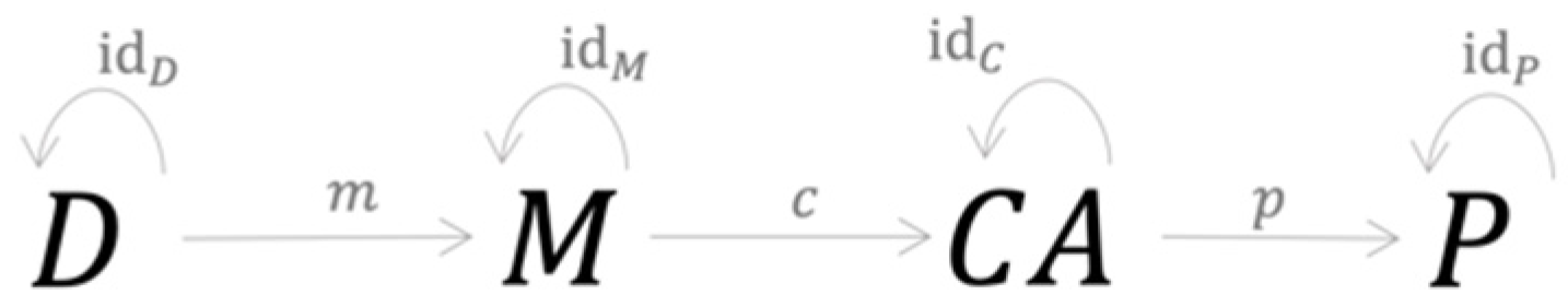
With the allocation and efficiency measures now defined, the conceptual approach to credit risk modeling, with a focus on optimal credit application, is proposed next. Its structure is presented by a category as shown in Figure 1.

At first sight, this category appears similar to the one representing current approaches to modeling credit risk,3 where object D represents a data structure that forms the basis of which specific data are collected, processed, analyzed and used in both the testing and training process, and object M represents model choice with the morphism m between D and M defined by a computational process that optimally maps the specific training dataset to a unique model. Nevertheless, substantial differences are apparent. First, the object C, representing the confusion matrix, is replaced by a new object CA, representing the predicted PDs and corresponding credit allocation amount. The morphism c now represents the Kelly betting strategy, and p represents the process of turning instances of CA into various measurements of performance, as proposed above, which constitute the elements of the object P. Based on this category framework, a computational implementation is developed, which is the subject of the next section.

2.3. Computational Implementation

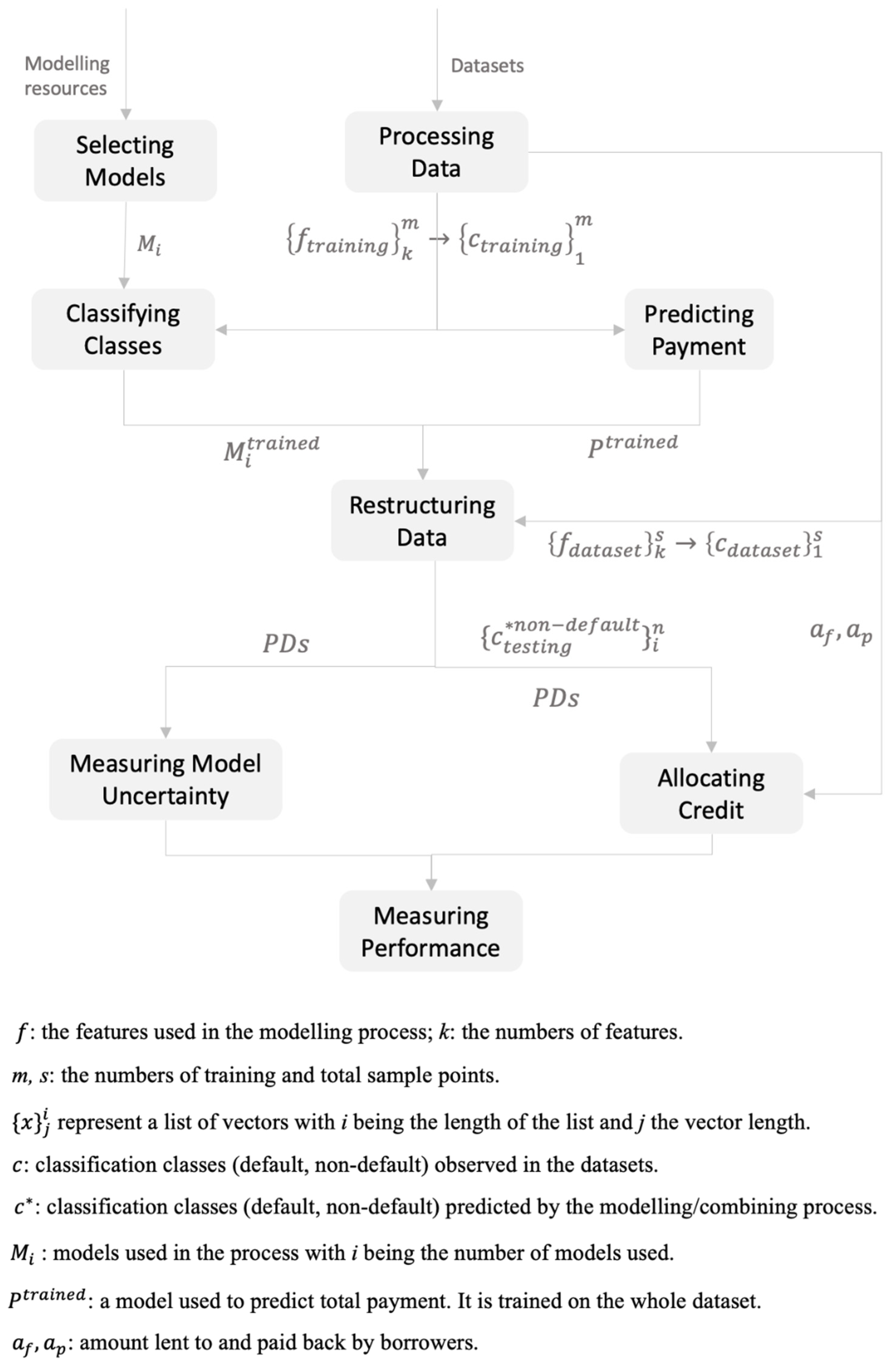
Four credit allocation systems are employed. The first credit allocation system is the adaptive Kelly strategy (‘Kelly Strategy’). Theoretically, the Kelly criterion states that the optimal strategy is to allocate a fraction of available capital to each borrower. This fraction should be equal to the difference between non-default probability (p) and default probability (q). Implicitly, this suggests that somehow in any proposed transaction, the amount of available capital is equal to the proposed borrowing amount. From a practical perspective, two considerations require attention: (i) lenders usually have more capital than what is needed in a proposed transaction; and (ii) PDs will likely carry different weights at different values. For example, a borrower with a PD of 0.8 will appear different from a borrower with a PD of 0.6, even though both may be classified as sound borrowers (“payers”). To make appropriate adjustments, a threshold is constructed based on the PDs estimated during the training process. The Kelly fraction (f) is set equal to the probability difference when the PD is less than a preassigned threshold value (5%), and equal to 1 when the PD is above this threshold. The funded amount therefore equals a fraction of the loan amount observed in the data. Total payment is estimated by a predictor trained on the full sample space before it is split into smaller subsets. This adaptive strategy performs an operation in the spirit of the bucketing process4 used to group PDs into clusters (Krink et al. 2007; Lyra et al. 2010; Tvrdik and Křivý 2015). The adaptive Kelly strategy, however, is simpler in its construction and has a sound theoretical basis.5 The second credit allocation system is the actual credit allocation observed directly from the data (‘System Actual Payment’). Here, all borrowers in the testing sample are accepted and fully funded, with the actual total loan payment observed directly from the data. The third credit allocation system (‘System’) is identical to the second one, except that the total payment amount is predicted from the borrowing amount with the same predictors employed as in the first allocation process to ensure consistency in the prediction process.6 The fourth and final credit allocation system (‘Base’) is where all borrowers appearing in the data are accepted and fully funded, regardless of whether they are classified as default or non-default by the model. This scenario is like the second allocation system (‘System Actual Payment’), except that the payment amount (rather than being observed from the actual data) is predicted as in the other approaches. A summary of all four credit allocation processes is provided in

Table 1. Summary of the credit allocation systems.

	Base	Kelly Strategy	System
Data Process	Two samples were randomly extracted from the original dataset. One of the samples was used to train the models, the other for testing. This process was repeated 100 times.	The same datasets were used to train and test the model.	The testing datasets were used only. No classifier is trained in this approach.
Model Selection	Nine standard classifiers available in the Mathematica software package: gradient boosted trees, logistic regression, Markov, nearest neighbors, random forest, support vector machine, neural network, decision tree and naive Bayes.	Identical classifiers were used.	No classifiers were used, with the results calculated directly from the actual data of funded amount and total payment.
Accepted Borrowers/Allocation Strategy	All borrowers in the test sample received full funding.	In the testing sample, only borrowers with difference between non-default probability and default probability of at least 5% are accepted. An adaptive Kelly strategy was used for determining the fraction of credit allocated to these borrowers.	All borrowers in the test sample received full funding. Actual credit allocation decisions are as reflected in the test data.
Performance Criteria	SCAP, ARC, AECE, AEVE and SEVE	SCAP, ARC, AECE and SEVE.	SCAP and ARC.
Significant Tests	Yes, to compare SCAP and ARC to systems with Kelly strategy. H1: The Kelly strategy is no better than other strategies. H2: The Kelly strategy is better than other strategies.	Yes, to compare SCAP and ARC to systems without Kelly strategy.	Yes, to compare SCAP and ARC to systems with Kelly strategy.
Payment Prediction	Yes, a predictive model was used to estimate loan payment.	Yes, a predictive model was used to estimate loan payment.	Yes, a predictive model was used to estimate loan payment for one approach (system). The other approach (system actual payment) used actual payment data to gauge how well the predictor worked.

(see Appendix A for flow chart).

For robustness, we conducted 100 simulations, where in each simulation two subsamples—one to train the model, the other for testing—were picked at random from the database. This process ensures that each subsample will have a different data structure regarding feature availability, especially categorical features. The performance results reported in the tables are thus the average of 100 simulations. The subsamples contain 20 percent of the original data, consisting of 268,676 data points, with the default to non-default ratio remaining around 4, identical to that observed in the full sample. Essentially, a scaled down sample of the original dataset is employed, with the structure of bad loans and good loans remaining the same. Nevertheless, this reduced sample is larger than any dataset employed in any previous studies on credit risk modeling (e.g., see Dastile et al. (2020)).

Nine classifiers were selected as the base models for default and payment prediction: logistic regression, nearest neighbors, random forest, gradient boosted trees, decision tree, support vector machine, Markov, naive Bayes and neural network. Details of these base models are provided in Tran et al. (2021).

Finally, the winning ratio (r) and the losing ratio (l) for the Kelly criterion were assumed to be constant over time and set equal to 1. In an actual credit risk allocation system, both r and l are less than 1 since the interest rate charged is typically much less than 100%, while borrowers usually pay some loan instalment prior to default. While deriving a correct value for the winning ratio is straightforward using existing lending rates, getting an accurate measure of l requires a model to estimate LGD. However, this requirement is well beyond the scope of this paper. First, setting the winning and losing ratios equal to 1 essentially assumes a long-term approach to allocating capital with a margin of safety. It is reasonable to assume that lenders prefer to make bets at least until their capital doubles, while preparing for total loss when default occurs. Second, current approaches to measuring LGD are essentially based on statistical methods that lack a sound conceptual framework (Calabrese and Zenga 2010; Chen et al. 2018; Zhang and Zhou 2018). Since the focus of this paper is on implementing a coherent computational model, statistical approaches that have no valid reasoning processes underlying them are avoided. Third, features needed for modeling LGD are not available in the peer-to-peer loan database considered in this paper. Fourth, the assumption of constant winning and losing ratio is realistic in terms of what is likely to happen in practice: lenders form expectations of the returns on their assets (loans) based on past experiences. These expectations are often captured in the notion of an approximate but sensible average value over time, rather than a stream of precise values that are sensitive to changing assumptions about the future. The notion of $r$ and $l$ capture such expectations given that Equations (1)–(5) have been developed from one loan to another within the context of $n$ loan decisions and then let $n$ increase to capture the notion of default and non-default probability through the frequency approach. Whilst relaxing the above assumption will give the modeler more control over the allocation process, it has no significant impact on the merits of the credit allocation strategy proposed in this paper.

3. Data

The modeling process was performed on the Lending Club’s personal loans dataset obtained from Kaggle (Lending Club 2020). Compared to the Lending Club dataset used in Teply and Polena (2020), the Kaggle dataset has more than 1.3 million sample points, is much larger in scope and has significantly more features, including total repayment by borrowers. Since the objective is credit allocation rather than credit classification, the larger dataset is preferred. Details of the features of the dataset used in both the classification and prediction models are provided in

Table 2. Summary of the Lending Club dataset used in both the classification and prediction models.

Sample Period	2007–2018
Original Sample Size	1,343,380
Filtered Samples	1,074,704
Filtering Criteria	Reduction size, current loans, loans in grace period, and sample with one of the training features having no or abnormal value.
Final Sample Size	268,676
Default Sample	53,638
Non-Default Sample	215,038
Classes	“Default” and “Non-default”
Number of Original Features	115
Number of Final Features	24
acc_now_delinq	Number of accounts on which the borrower is now delinquent.
annual_inc	Self-reported annual income provided by the borrower during registration.
chargeoff _within12mths	Number of charge-offs within 12 months.
delinq_2yrs	The number of 30+ days past-due incidences of delinquency in the borrower’s credit file for the past 2 years.
delinq_amnt	Past-due amount owed for the accounts on which the borrower is now delinquent.
Dti	A ratio calculated using the borrower’s total monthly debt payments on the total debt obligations, excluding mortgage and the requested LC loan, divided by the borrower’s self-reported monthly income.
home_ownership	Home ownership status provided by the borrower during registration or obtained from the credit report.
inq_last_6mths	The number of inquiries in past 6 months (excluding auto and mortgage inquiries).
loan_amnt	Listed amount of the loan applied for by the borrowers.
funded_amnt	Actual amount received by the borrowers.
open_acc	Number of open credit lines in the borrower’s credit file.
pub_rec	Number of derogatory public records.
pub_rec_bankruptcies	Number of public record bankruptcies.
purpose	Category provided by the borrower for the loan request.
revol_util	Revolving line utilization rate, or the amount of credit the borrower is using relative to all available revolving credit.
term	Number of payments on the loan. Values are in months and can be either 36 or 60.
tax_liens	Number of tax liens.
total_acc	Total number of credit lines currently in the borrower’s credit file.
verication_status	Indicates if income was verified (1) by LC or not verified (0).
loan_status	Final status of loan has labelled outcome. “Non-default” for fully paid loans and “Default” for charged-off loans.
emp_length	Number of years in employment represented by continues variable going from 0 to 10.
earliest_cr_line	Number of years since the first credit line has been opened.
fico_range_low	The low FICO value.
fico_rangee_high	The high FICO value.

.

4. Empirical Results

Table 3. Capital allocation performance.

Measures/Models	Logistic Regression	Nearest Neighbors	Random Forest	Gradient Boosted Trees	Decision Tree	Support Vector Machine	Markov	Naive Bayes	Neural Network
SCAP—System Actual Payment	2.90%	2.90%	2.90%	2.90%	2.90%	2.90%	2.90%	2.90%	2.90%
SCAP—System	3.10%	3.10%	3.10%	3.10%	3.10%	3.10%	3.10%	3.10%	3.10%
SCAP—Base	3.60%	3.20%	3.40%	3.40%	3.80%	3.20%	3.30%	4.20%	3.60%
SCAP—Kelly Strategy	14.30%	11.30%	16.10%	14.30%	6.70%	5.50%	13.50%	13.70%	14.30%
ARC—System Actual Payment	91.643	91.643	91.643	91.643	91.643	91.643	91.643	91.643	91.643
ARC—System	119.488	119.488	119.488	119.488	119.488	119.488	119.488	119.488	119.488
ARC—Base	128.802	120.142	123.003	123.27	113.923	120.484	120.391	124.565	127.714
ARC—Kelly Strategy	3763.89	650.865	1787	4821.15	209.044	207.813	1427.38	3216.45	3642.58
AEC—Base	1715.76	1775.4	2302.67	1734.33	430.265	853.052	1705.24	991.763	1606.6
AEC—Kelly Strategy	1715.76	1775.4	2295.6	1734.33	411.466	853.052	1705.24	991.763	1606.6
AEV—Base	0.658	0.661	0.875	0.659	0.197	0.318	0.648	0.449	0.623
AEV—Kelly Strategy	0.658	0.661	0.874	0.659	0.19	0.318	0.648	0.449	0.623

Notes: Reported are the mean SCAP, ARC, AEC and AEV values computed over 100 simulations. SCAP = system credit allocation performance, ARC = area under the return curve, AEC = area under the entropy curve and AEV = average entropy value. The credit allocation approaches are described in Table 1.

reports the mean values of the capital allocation effectiveness (SCAP and ARC) computed over 100 simulations. The results show that the credit allocation system based on the Kelly strategy strongly outperforms the other approaches on both performance criteria across all base models. For both the support vector machine and decision tree classifiers, the Kelly strategy shows an 80% increase in SCAP when compared to the alternative credit allocation systems. All other classifiers show a minimum 3-fold increase in SCAP for the Kelly strategy. The random forest model delivers the best performance, with a more than 4-fold increase in SCAP for the Kelly strategy. Recall that SCAP considers not only investment return but also the amount of credit allocated to borrowers. Similar increases in performance are observed for the ARC measure across all classifiers—the support vector machine and decision tree classifiers show an 80% increase in performance for the Kelly strategy, with all other classifiers delivering at least a 5-fold increase in ARC. Univariate tests of mean difference in performance of the Kelly strategy vs. alternative credit allocation systems reported in

Table 4. Univariate tests of mean difference in performance of the Kelly strategy vs. alternative strategies.

Measures/Models	Logistic Regression	Nearest Neighbors	Random Forest	Gradient Boosted Trees	Decision Tree	Support Vector Machine	Markov	Naive Bayes	Neural Network
SCAP—System Actual Payment	<0.01	<0.01	<0.01	<0.01	<0.01	<0.01	<0.01	<0.01	<0.01
SCAP—System	<0.01	<0.01	<0.01	<0.01	<0.01	<0.01	<0.01	<0.01	<0.01
SCAP—Base Models	<0.01	<0.01	<0.01	<0.01	<0.01	<0.01	<0.01	<0.01	<0.01
ARC—System Actual Payment	<0.01	<0.01	<0.01	<0.01	<0.01	<0.01	<0.01	<0.01	<0.01
ARC—System	<0.01	<0.01	<0.01	<0.01	<0.01	<0.01	<0.01	<0.01	<0.01
ARC—Base Models	<0.01	<0.01	<0.01	<0.01	<0.01	<0.01	<0.01	<0.01	<0.01

Notes: SCAP = system credit allocation performance, ARC = area under the return curve. H1: The Kelly strategy is no better than other strategies. H2: The Kelly strategy is better than other strategies. Reported are the p-values. The algorithm automatically selects the most optimal test (Mann–Whitney or t-test) that fits the simulation data. The credit allocation approaches are described in Table 1.

confirm these results.

There are two observations that warrant explanation. First, both AEC and AEV values are nearly identical for all classifiers employed, irrespective of whether the Kelly strategy is used or not. This can be explained by the fact that both scenarios use the same set of accepted borrowers and thus the same PDs to compute entropy.7 Second, for the Kelly strategy, the performance across the classification models varies substantially. For example, at one end of the performance spectrum is random forest, with a SCAP of 16.1%, ARC of 1787, AEC of 2295 and AEV of 0.874. At the other end is support vector machine, with a SCAP of 5.5%, ARC of 207.813, AEC of 853.02 and AEV of 0.318. This wide difference in performance can be explained by the fact that each classification model uses a different set of Kelly fractions, as reflected by the differences in AEC and AEV values. For all other allocation strategies, the full amount requested is granted, regardless of the value of AEC or AEV, thus resulting in similar SCAP and ARC values.

Table 5. Efficiency in processing information.

Measures/Models	Logistic Regression	Nearest Neighbors	Random Forest	Gradient Boosted Trees	Decision Tree	Support Vector Machine	Markov	Naive Bayes	Neural Network
SEVE—No Kelly Strategy	0.055	0.048	0.039	0.052	0.196	0.103	0.051	0.095	0.058
SEVE—Kelly Strategy	0.219	0.171	0.184	0.216	0.353	0.174	0.209	0.304	0.228
AECE—No Kelly Strategy	0.075	0.068	0.053	0.072	0.267	0.145	0.071	0.128	0.080
AECE- Kelly Strategy	2.165	0.369	0.776	2.769	0.510	0.248	0.833	3.163	2.222
Significance Test (p-value)—SEVE	<0.001	<0.001	<0.001	<0.001	<0.001	<0.001	<0.001	<0.001	<0.001
Significance Test (p-value)—AECE	<0.001	<0.001	<0.001	<0.001	<0.001	<0.001	<0.001	<0.001	<0.001

Notes: Reported are the mean SECE and AECE values computed over 100 simulations. SEVE = system entropy value efficiency, AECE = area under the entropy curve efficiency. H1: The Kelly strategy is no better than other strategies. H2: The Kelly strategy is better than other strategies. The algorithm automatically selects the most optimal test (Mann–Whitney or T-test) that fits the simulation data. The credit allocation approaches are described in Table 1.

reports the mean values of the efficiency in processing metrics (AECE and SEVE) computed over 100 simulations. The results show that the Kelly strategy utilizes information embedded in the entropy value more efficiently than the alternative credit allocation systems, thus providing better performance per unit of information. The statistical significance tests (p < 0.01) reject the null that the credit allocation system based on the Kelly strategy processes information with similar efficiency as the alternative credit allocation systems. While each model has a different level of efficiency in processing credit risk information, the performance gains of the Kelly strategy are consistent across classifiers and data environments. In sum, the results suggest that the Kelly strategy is robust to the choice of classifier, providing a more efficient credit allocation system.

5. Conclusions

This paper outlines the merits of designing a credit risk model with a focus on optimal credit allocation rather than just dichotomous default classification. Predicting a borrower’s PD is a key requirement of any credit risk model but turning it into labeled classes immediately leads to issues in performance measurement. The decoupling of modeling PDs from modeling credit allocation, as is often seen in the credit risk literature makes it difficult to understand how credit should be allocated optimally given a borrower’s default probability.

The credit allocation strategy proposed in this paper addressed this issue by providing two constructs. First, the connection between PDs and optimal credit allocation was established through a conceptual construct called the Kelly criterion. Second, conflicting performance criteria in dichotomous classification were replaced with coherent criteria for judging the performance of credit allocation system. The whole process was guided by a new perspective on modeling credit risk based on sound structures derived from category theory. Extensive testing on various data environments provided results that confirm the soundness of the conceptual constructs proposed. For all classifiers employed, the Kelly strategy consistently outperformed alternative credit allocation systems with unparalleled efficiency in processing information.

Even though several aspects of the modeling process were not optimized, such as the Kelly threshold, the allocation strategy proposed performed remarkably well. This opens possibilities for further improvement in performance. In particular, the findings point to two key considerations for the design of an effective allocation system in practice. First, the equivalence concept proposed by category theory and detailed in an earlier paper (Tran et al. 2021), provides a concrete basis for reasoning that combining several models would be a better way to construct optimal Kelly fractions. Confirmation of this proposition would require a level of analysis beyond the scope of the current paper. Second, the Kelly strategy requires a credit allocation system capable of distributing fractions of a loan among different lenders in concurrent state. In other words, the technology infrastructure required for such a system must be able to handle large scale concurrent computation tasks related to fractional credit allocation and back-end operations, such as accounting and transaction tracking. Conceptual structures in optimal credit allocation could be a key consideration in the design of such an infrastructure. Viewing credit risk modeling as an allocation challenge will eventually lead to better understanding of how the task could be implemented effectively and efficiently in practice. Likewise, discussions regarding a framework for ongoing diagnosis of clients’ credit health, a topic that plays an important role in credit risk modeling but so far been avoided, are also worthwhile. Another interesting direction worthy of exploring further is identification of the source of the outperformance of the Kelly criterion—is it due to large allocation being given to high-risk borrowers who may not be offered a loan in practice? To find an answer would require additional data on borrowers who were initially rejected loans, being classified as “non-payers” during the application process. We will leave these suggestions for others to pursue.

References

- Abdou, Hussain, and John Pointon. 2011. Credit scoring, statistical techniques and evaluation criteria: A review of the literature. Intelligent Systems in Accounting, Finance and Management 18: 59–88. [Google Scholar] [CrossRef] [Green Version]
- Altman, Edward I. 1968. Financial ratios, discriminant analysis and the prediction of corporate bankruptcy. Journal of Finance 23: 589–609. [Google Scholar] [CrossRef]
- Byanjankar, Ajay, and Markus Viljanen. 2019. Predicting expected profit in ongoing peer-to-peer loans with survival analysis-based profit scoring. In Intelligent Decision Technologies. Berlin and Heidelberg: Springer, pp. 15–26. [Google Scholar] [CrossRef]
- Calabrese, Raffaella, and Michele Zenga. 2010. Bank loan recovery rates: Measuring and nonparametric density estimation. Journal of Banking & Finance 34: 903–11. [Google Scholar] [CrossRef]
- Chen, Jian, Yao Shen, and Riaz Ali. 2018. Credit Card Fraud Detection Using Sparse Autoencoder and Generative Adversarial Network. Paper presented at 2018 IEEE 9th Annual Information Technology, Electronics and Mobile Communication Conference (IEMCON), Vancouver, BC, Canada, November 1–3; pp. 1054–59. [Google Scholar] [CrossRef]
- Dastile, Xolani, Turgay Celik, and Moshe Potsane. 2020. Statistical and machine learning models in credit scoring: A systematic literature survey. Applied Soft Computing 91: 106263. [Google Scholar] [CrossRef]
- Eleftherios, Vlachostergios. 2019. Basel risk weight functions and forward-looking expected credit losses. Journal of Credit Risk 14: 29–42. [Google Scholar] [CrossRef]
- Hwang, Ruey-Ching, Chih-Kang Chu, and Kaizhi Yu. 2020. Predicting the loss given default distribution with the zero-inflated censored beta-mixture regression that allows probability masses and bimodality. Journal of Financial Services Research 59: 143–72. [Google Scholar] [CrossRef]
- Izzi, Luisa, Gianluca Oricchio, and Laura Vitale. 2012. Basel III Credit Rating Systems: An Applied Guide to Quantitative and Qualitative Models. London: Palgrave MacMillan, ISBN 978-0-230-36118-8. [Google Scholar]
- Jobst, Rainer, Ralf Kellner, and Daniel Rösch. 2020. Bayesian loss given default estimation for European sovereign bonds. International Journal of Forecasting 36: 1073–91. [Google Scholar] [CrossRef]
- Kaposty, Florian, Johannes Kriebel, and Matthias Löderbusch. 2020. Predicting loss given default in leasing: A closer look at models and variable selection. International Journal of Forecasting 36: 248–66. [Google Scholar] [CrossRef]
- Kelly, John L. 1956. A new interpretation of information rate. Bell Labs Technical Journal 35: 917–26. [Google Scholar] [CrossRef]
- Krink, Thiemo, Sandra Paterlini, and Andrea Resti. 2007. Using differential evolution to improve the accuracy of bank rating systems. Computational Statistics & Data Analysis 52: 68–87. [Google Scholar]
- Lending Club. 2020. Peer-to-Peer Loans Data. Available online: https://www.kaggle.com/wordsforthewise/lending-club (accessed on 24 November 2020).
- Lessmann, Stefan, Bart Baesens, Hsin-Vonn Seow, and Lyn C. Thomas. 2015. Benchmarking state-of-the-art classification algorithms for credit scoring: An update of research. European Journal of Operational Research 247: 124–36. [Google Scholar] [CrossRef] [Green Version]
- Lyra, Marianna, Johannes Paha, Sandra Paterlini, and Peter Winker. 2010. Optimization heuristics for determining internal rating grading scales. Computational Statistics & Data Analysis 54: 2693–706. [Google Scholar]
- MacLean, Leonard C., Edward O. Thorp, and William T. Ziemba. 2011. Long-term capital growth: The good and bad properties of the Kelly and fractional Kelly capital growth criteria. Quantitative Finance 10: 681–87. [Google Scholar] [CrossRef]
- Mathur, Ike, and Isaac Marcelin. 2014. Unlocking credit. Contemporary Studies in Economic and Financial Analysis 96: 221–52. [Google Scholar]
- Papoušková, Monika, and Petr Hajek. 2019. Modeling loss given default in peer-to-peer lending using random forests. In Intelligent Decision Technologies. Berlin and Heidelberg: Springer, pp. 133–41. [Google Scholar]
- Rotando, Louis M., and Edward O. Thorp. 1992. The Kelly criterion and the stock market. American Mathematical Monthly 99: 922–31. [Google Scholar] [CrossRef]
- Schutte, Willem D., Tanja Verster, Derek Doody, Helgard Raubenheimer, and Peet J. Coetzee. 2020. A proposed benchmark model using a modularised approach to calculate IFRS 9 expected credit loss. Cogent Economics & Finance 8: 1735681. [Google Scholar]
- Shannon, Claude E. 1948. A mathematical theory of communication. The Bell System Technical Journal 27: 379–423. [Google Scholar] [CrossRef] [Green Version]
- Srivastava, Vikas, and Surya Dashottar. 2020. Default probability assessment for project finance bank loans and Basel regulations: Searching for a new paradigm. Journal of Structured Finance 25: 41–53. [Google Scholar] [CrossRef]
- Stein, Roger M. 2005. The relationship between default prediction and lending profits: Integrating ROC analysis and loan pricing, bank runs. Journal of Banking and Finance 29: 1213–36. [Google Scholar] [CrossRef]
- Teply, Petr, and Michal Polena. 2020. Best classification algorithms in peer-to-peer lending. North American Journal of Economics and Finance 51: 100904. [Google Scholar] [CrossRef]
- Tran, Cao S., Dan Nicolau, Richi Nayak, and Peter Verhoeven. 2021. Modeling credit risk: A category theory perspective. Journal of Risk and Financial Management 14: 298. [Google Scholar] [CrossRef]
- Tvrdik, Josef, and Ivan Křivý. 2015. Hybrid differential evolution algorithm for optimal clustering. Applied Soft Computing 35: 502–12. [Google Scholar] [CrossRef]
- Zhang, Xingzhi, and Zhuriong Zhou. 2018. Credit scoring model based on kernel density estimation and support vector machine for group feature selection. Paper presented at 2018 International Conference on Advances in Computing, Communications and Informatics (ICACCI), Bangalore, India, September 19–22; pp. 1829–36. [Google Scholar] [CrossRef]
Figure 1.
Categorical construct of credit risk modeling based on optimal capital allocation.