
The Time-Varying Relation between Stock Returns and Monetary Variables


Division of Accounting and Finance, University of Stirling, Stirling FK9 4LA, UK
J. Risk Financial Manag. 2022, 15(1), 9; https://0-doi-org.brum.beds.ac.uk/10.3390/jrfm15010009
Submission received: 14 October 2021
/
Revised: 25 November 2021
/
Accepted: 3 December 2021
/
Published: 31 December 2021
(This article belongs to the Special Issue Economic Forecasting)
Abstract
:The nature of the relation between stock returns and the three monetary variables of interest rates (bond yields), inflation and money supply growth, while oft studied, is one that remains unclear. We argue that the nature of the relation changes over time, and this variation is largely driven by shocks, with a change in risk associated with each variable shifting the pattern of behaviour. We show a change in the correlation between each of the three variables with stock returns. Notably, a predominantly negative correlation with bond yields and inflation becomes positive, while the opposite is true for money supply growth. The shift begins with the bursting of the dotcom bubble but is exacerbated by the financial crisis. Results of predictive regressions for stock returns also indicate a switch in behaviour. Predominantly negative predictive power switches temporarily to positive around economic shocks. This suggests that higher yields, inflation and money growth typically depress returns but support the market during periods of stress. However, after the financial crisis, higher inflation and money growth exhibit persistent positive predictive power and suggest a change in the risk perception of higher values.
Keywords:
stock returns; interest rates; inflation; money supply; time-variation; correlation; predictabilityJEL:
C22; G121. Introduction
The nature of the relation between stock returns and three monetary variables, interest rates, inflation and money supply growth, has changed over the past 20 years (see, for example, Campbell and Ammer 1993; Rankin and Shah Idil 2014; Fan and Mitchell 2017; McMillan 2017). This paper, therefore, aims to examine these changing relations. We document, first, how the nature of the relations has changed, for example, shifts within the sign of the correlations, and second, we seek to explain the reasons for such change. We further consider the potential for changing parameter values in a predictive regression for stock returns.
Movements in stock returns are determined by changes in discounted cashflows (e.g., Campbell and Shiller 1988). Hence, the link between these three variables with stocks is in how they affect both cashflow and the discount rate. Notably, changes in each variable have implications for subsequent economic performance and the risk premium attached to stocks and thus should exhibit predictive power. Hence, part of our question concerns the risk-related implications of each variable and whether this has changed. Knowledge of these changing relations is crucial for both asset pricing and the conduct of portfolio management, implying time-varying behaviour between stocks and key economic variables.
The relation between stock returns and bond yields is one that is well researched, with a change in their correlation identified. Notably, several papers report a change in the sign of the stock and bond correlation and condition this change on a range of macroeconomic and financial variables (e.g., Andersson et al. 2008; Baele et al. 2010; Viceira 2012; Aslanidis and Christiansen 2012, 2014; Aslanidis et al. 2019). The evidence typically identifies a change around the time of the dotcom crash (2000) and links this behaviour to a flight-to-safety phenomenon, which is combined with a period of low interest rates. Li (2002) develops a theoretical model that links the sign of the correlation to the source of shocks, while the above noted studies use empirical frameworks to identify variables that may explain the correlation.
In terms of the relation between stock returns and inflation, likewise, there is an ongoing debate about its nature and one that extends back over a longer period. Fisher (1930) argues in favour of a positive relation to maintain the real value of stock returns, while Bodie (1976) applies a similar, inflation hedge argument. Fama (1981), in contrast, argues in favour of a negative relation arising through the proxy hypothesis with stock returns driven down as higher inflation leads to poorer expected economic conditions. Indeed, notwithstanding that evidence for both a positive and negative relation is presented, there exists greater support for a negative one (e.g., Fama and Schwert 1977; Barnes 1999), while an extensive review is provided by Madadpour and Asgari (2019).1
Regarding money supply, again, the literature provides a mixed picture, with the relation dependent on the expected future impact of a change in money supply on economic conditions and interest rates.2 Of note, Sellin (2001) provides a review of the literature linking monetary growth and stock returns and details the potential for positive and negative influences. A positive relation can arise whereby looser current monetary policy will give rise to expectations of a future tightening that will lead to higher interest rates and, through the discount rate, higher future stock returns (lower prices). Equally, higher interest rates will depress economic activity and put further downward pressure on current stock prices. The negative predictive relation can be explained through a decreased in the risk premium, which leads to a higher current price and lower expected return. An increase in money supply leads to lower interest rates and improved economic expectations, higher expected earnings and lower macroeconomic risk. Thus, whether money supply growth has a positive or negative effect on stock returns largely rests on its effect on expectations and the implications for future economic activity and risk. In recent work, McMillan (2017) indicates that money supply growth has a negative predictive relation for stock returns, and this is driven by higher money supply growth leading to lower risk and improving economic conditions.
As indicated above, while research into the stock and bond relation has continued apace, the relation regarding inflation and money supply growth, while a recurring theme, has been more ignored in recent times, and notably so for money supply. This may have occurred as, on the one hand, central banks have dropped money supply targets with interest rates adjusted to meet inflation targets that now dominate monetary policy considerations, and, on the other hand, bond market considerations more directly interact with stocks in portfolio building. However, the past 20 years have witnessed significant economic turmoil, from the highs and lows of the dotcom bubble to the financial crisis of 2007–2009 and the COVID-19 pandemic throughout 2020 and beyond. This suggests that a re-examination of the relations between stock returns and these three monetary variables is needed. Thus, we consider the nature of the relation between stocks and these variables, examining whether the magnitude and sign of any relation has changed: notably, whether the correlation between stocks and bonds returned to its pre-2000 state or the pattern that emerged since this date remains, and equally, whether the negative relation with inflation and money supply growth continues to hold.
Moreover, understanding the nature and drivers of these relations is important for both investors and policymakers. Since the bursting of the dotcom bubble, interest rates have reached unprecedented lows, which has been exacerbated first by the financial crisis and then the COVID-19 pandemic. The result of this is 10-year Treasury bond yields below 2.5% for most of the past 10 years (and 3-month bills below 0.5%). Further to this, while the quantitative easing (QE) that followed the financial crisis saw annual increases in M2 growth of around 10%, following COVID-19 induced QE, annual M2 growth increased by over 20%. Such changes are likely to an impact the nature of relations between the variables and affect investors.
Our results indicate that both the correlation and predictive relation of interest rates, inflation and money supply growth with stock returns change over the sample period. The correlation involving interest rates and inflation is predominately negative from the start of the sample before becoming primarily positive after 2000, while the reverse case is reported for money supply growth. The three monetary variables have a largely negative predictive relation, where increases in each depress stock return. Around crisis periods, however, the predictive relation temporarily switches to positive, with higher values supporting the market. Moreover, after the financial crisis period, this switch becomes more persistent for inflation and money supply growth. This indicates a change in the risk perception of higher inflation and money supply growth, with increases suggesting improving future economic conditions.
2. Background
In understanding why stock returns move, and thus how the three monetary variables link, we consider the standard theoretical present value model based on Campbell and Shiller (1988) and expanded on by Lamont (1998) and Bali et al. (2008). Log stock returns (rt) are given by:
with Pt and Dt representing prices and dividends. Using an approximation around a first-order Taylor expansion, Equation (1) becomes:3
where k is a linearisation parameter and ρ a constant discount factor.4 Given Equation (2), Lamont shows that the time t expectation of time t + 1 returns can be written as:
This equation notes that expected returns are negatively related to the current price and are higher with higher expected future dividends (cashflow) and future returns (risk premium). Each of the interest rate, inflation and money supply growth variables can affect stock returns through their impact on expected future economic conditions and thus cashflow and risk. Moreover, the relation in Equation (3) also demonstrates the potential for confounding effects. For example, higher interest rates and inflation can signal poorer economic conditions with lower cashflow and lower stock returns but equally a higher risk premium and returns.
In considering the relation between stocks and bonds, the literature is predominantly couched in the correlation and for which research has identified both positive and negative periods. In identifying the sign of correlations, care needs to be taken regarding whether we examine the correlation between stock and bond returns (based on a price index) or stock returns with bond yields. The nature of these two correlations is often the opposite. For example, a rise in the bond yield will lead to a fall in the bond price and so a negative bond return. Equally, a typical assumption is that higher interest rates lead to lower stock prices as future cashflows are discounted at a higher rate. Thus, the correlation between the two returns is positive, while the stock return and bond yield correlation is negative. Within the literature, Barsky (1989), Shiller and Beltratti (1992) and Campbell and Ammer (1993) all highlight a positive correlation between stock and bond returns, while a negative correlation linked to flight-to-safety is noted by, for example, Gulko (2002), Connolly et al. (2005, 2007) and Andersson et al. (2008).5 As an example of the changing correlation, Gregoriou et al. (2009) note that stock prices fell with interest rates during the financial crisis, reversing the usual expectation. They argue that the lower interest rates signalled weaker economic conditions.
In seeking to explain the change in correlation, the literature identifies several variables that proxy for risk factors that may drive such dynamics. As noted, discussion typically focuses on the flight-to-safety phenomena as main cause of change to the correlation. Thus, a series of papers consider a range of macroeconomic and financial variables that explain the change in the stock and bond correlation through their links to wider economic risk.
Li (2002), in developing a theoretical model to link stock and bond returns, argues that while interest rate shocks will lead to a positive correlation, dividend and inflation shocks negatively affect the correlation. Baele et al. (2010) consider inflation and interest rates for the stock and bond correlation and include an output measure. Likewise, for the stock and bond correlation, Aslanidis and Christiansen (2012, 2014) use interest rates and inflation. They also include the dividend/price ratio (and other valuation-related variables). Viceira (2012) also considers interest rate and inflation variables together with the asset returns and macroeconomic variables (they include consumption growth instead of output growth). Aslanidis et al. (2019) include interest rates, a measure of output growth and measures of financial conditions and policy uncertainty.
In considering the stock return and inflation and stock return and money supply growth relations and the factors that affect them, inevitably the same proxies for economic risk are important. The literature regarding inflation began with the work of Fisher (1930) who argues for a positive relation between stock returns and inflation. In contrast, Fama (1981) suggests a negative correlation between stock returns and inflation as higher inflation signals lower economic growth. The subsequent literature has tended to favour a negative relation, while the extent to which stocks returns might respond negatively to higher inflation is likely to depend on the state of the economic, and interest rate, cycle. Stulz (1986) argues that higher inflation is associated with a lower real interest rate and, equally, stock return. In contrast, Fisher (1930) suggests that to maintain the real return on stocks, the return should move in unison with inflation. Bodie (1976) likewise supports an inflation hedge argument, where investors are compensated for higher inflation through higher stock returns. In considering these opposing views, Söderlind (1998) argues that the correlation depends on whether the central bank is targeting output growth or inflation. This link with monetary policy is also commented upon by Geske and Roll (1983) and Kaul (1987). Notwithstanding this, some work argues that a positive relation can exist, although this typically emerges only when examined over a longer horizon (e.g., Boudoukh and Richardson 1993; Schotman and Schweitzer 2000). Further work considers the distribution of returns using a quantile approach (Alagidede and Panagiotidis 2012) and reports a positive relation at higher quantiles.
The sign of the stock returns and monetary growth relation is similarly unclear.6 Here, again we can consider the potentially confounding effects of the cashflow and the discount rate avenues. A positive relation with money supply growth can arise where higher growth improves economic conditions and boosts expected cashflows, or where higher growth increases expected future inflation, leading to worsening economic conditions and a higher risk premium and discount rate. Thus, we have confounding effects where a higher money supply could affect corporate earnings (e.g., lower interest rates leading to higher consumption and investment) or the riskiness of those earnings (e.g., affecting the risk premium by which future cashflows are discounted).
Moreover, a change in money supply is linked to both interest rates and inflation, and so we can see how the three variables interact with stocks. At a basic level, the dividend discount model suggests that an increase in money supply leads to a decrease in interest rates (Friedman 1961). This can lower the discount rate and lead to an increase in the current stock price. Lower interest rates that decrease the risk-free component of the discount rate, may also decrease the risk premium component, as lower interest rates could signal lower macroeconomic risk, an increase in expected future economic activity and correspondingly corporate earnings. This will result in a negative relation with future stock returns.
Equally, building on the argument of Fama (1981) for inflation, higher money supply will signal higher expected inflation and a decline in stock returns. From a risk premium perspective, Sellin (2001) argues that an expectation of a tightening of future monetary policy will lead to higher current interest rates (and risk premium) and higher stock returns (lower prices). Higher interest rates may also depress economic activity and lead to further downward pressure on current stock prices. Recent evidence suggests that monetary policy primarily operates through the risk channel (see, for example, Hanson and Stein 2015; Gertler and Karadi 2015).
Cornell (1983) focuses on the risk premium effect of an increase in the money supply and supports a positive relation with stock returns. Cornell argues that holding money as opposed to alternate assets is directly proportional to risk and risk aversion. An unexpected increase in money supply indicates higher money demand, which suggests an increase in risk. As such, investors demand a higher risk premium for holding stocks, causing prices to fall, and making them less attractive. In contrast, Bernanke and Kuttner (2005) argue that money supply changes and the risk premium vary inversely. A tightening of money supply increases the risk premium required to compensate investors for holding risky assets as it indicates a slowing of economic activity. Here, investors bear more risk and demand a higher risk premium to hold stocks. This risk premium lowers the price of the stock.
Overall, the evidence on the nature of the relations is mixed. For each of bond yields, inflation and money supply growth, there is evidence of a positive and negative relation with stock returns. A higher money supply leads to lower interest rates, higher stock prices and lower stock returns. However, higher money supply can also lead to higher inflation and interest rates, a lower stock price and higher returns. The most recent evidence for stock returns points towards a positive relation with bond yields and a negative one with inflation and money supply growth. This paper therefore seeks to reconsider the above views and examine the nature of both the correlation and predictive relations over the most recent period including the COVID-19 pandemic, notably asking whether a change in the nature of macroeconomic risk affects these relations.
3. Data and Correlations
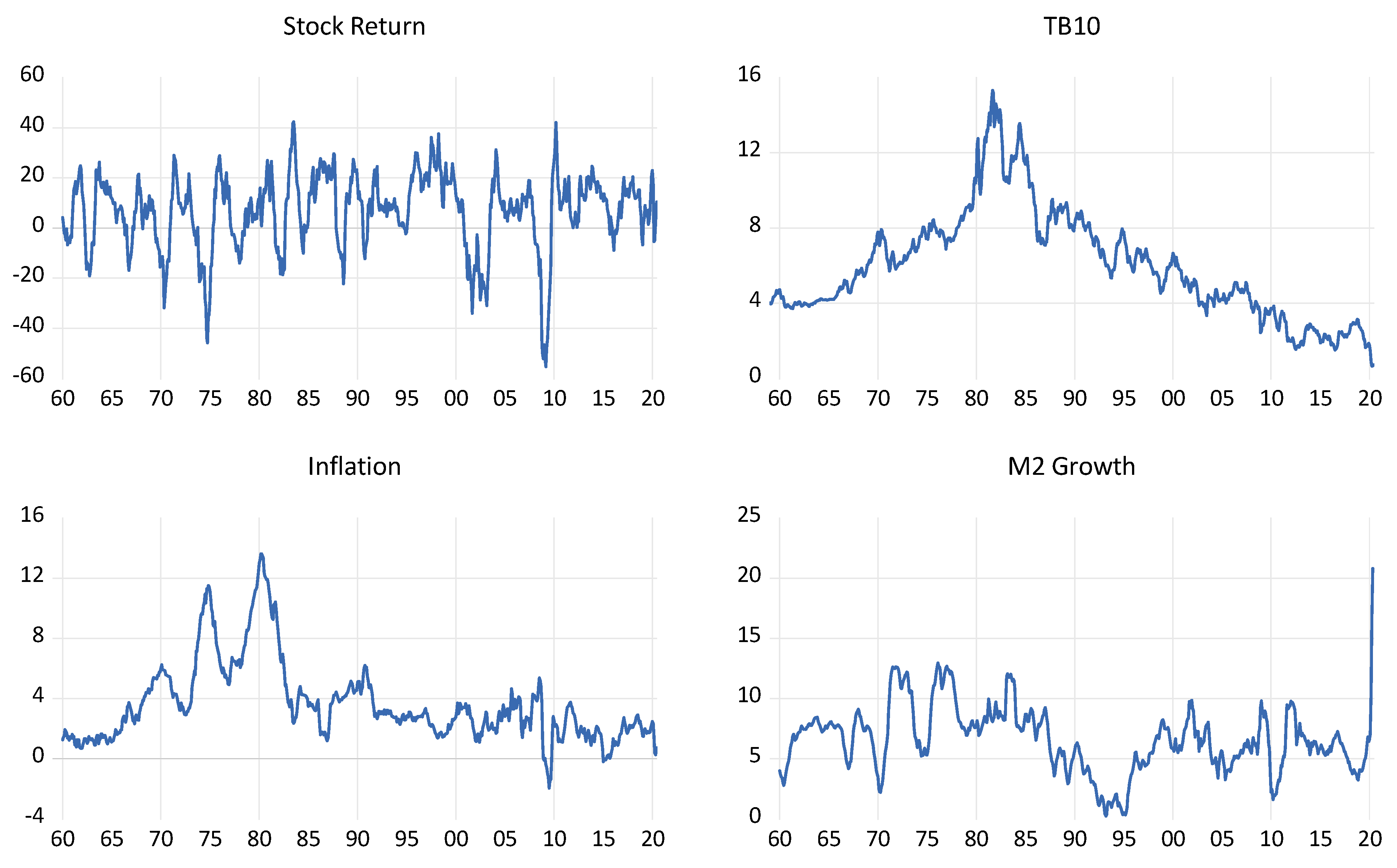
We obtained monthly data for the S&P500 index, 10-Year Treasury bonds (TB10), the consumer price index (CPI) and M2 money supply over the period from 1959M1 to 2020M6. The stock price data are from the website of Shiller, while the remaining data are taken from the Federal Reserve FRED database. Figure 1 presents the annualised return/growth rates for the stock index, CPI (inflation) and M2 series and the level of the TB10, while Table 1 presents both monthly and annualised summary statistics. Table 1 also presents the monthly and annual correlations, although our primary focus is on the stock return correlations.
While the data are well known, from Figure 1, we can observe significant market drops in the early 1970s, including those associated with the oil price shock of 1974, two notable bear markets in the 1980s including the October 1987 crash, the dotcom crash of the early 2000s and the financial-crisis-related crash of 2008–2009. As the data are annualised, the COVID-19-related crash is not evident here; however, in the monthly data, we can observe a 20% fall in March of 2020. In the other series, we can see the secular decline in interest rates since the highs of the early 1980s and reaching unprecedented lows following, first, the financial crisis and then the COVID-19 pandemic. In the inflation series, we see the highs that were spurred on by the oil price shocks of the 1970s. The 1980s were marked by policy designed to control inflation before a period of general price stability in the 1990s and 2000s, which appeared to end just prior to the financial crisis, with inflation in the post-crisis period subdued. The most notable aspect regarding M2 money supply growth is the huge increase associated with the COVID-19 pandemic, dwarfing previous increases.
Regarding Table 1, the summary statistics present no unusual characteristics, so we focus on the correlations reported in the lower panel of the table. We report correlations for the monthly (upper right triangle) and annualised (lower left triangle) data. Our primary interest concerns the correlations with stock returns. We can see that the value of both the monthly and annualised stock return correlations are all close to zero. This result covers the full sample period and so may arise because the correlation is near zero or because this masks greater variation in the correlation, which traverses zero. Moreover, these are (very) mildly negative for the monthly frequency and positive for the annual. The only exception is the annual correlation with inflation, which exhibits a slightly larger negative value. Regarding the correlations across the other variables, the TB10 and inflation correlation exhibits the largest positive values at both the monthly and annual frequencies, while the annual TB10 and inflation correlations with M2 growth are mildly positive.
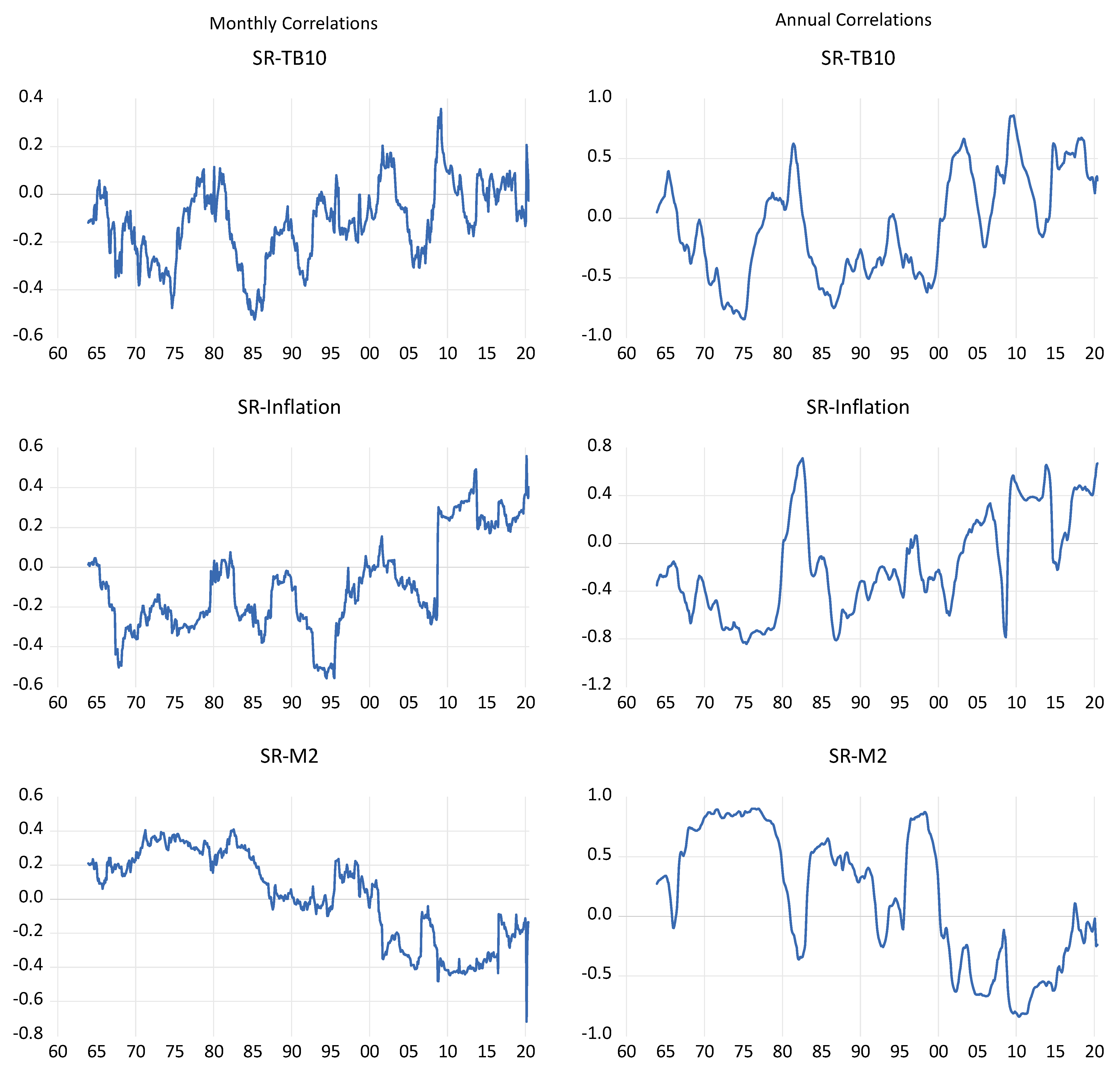
To consider whether the correlation coefficients for the whole sample are representative of the contemporary relation between stock returns and the three monetary variables, Figure 2 plots the 5-year rolling correlations between stock returns and TB10, inflation and M2 growth over both the monthly and annualised frequencies. Across both frequencies the results are similar, and thus we discuss them concurrently. The correlation between stock returns and TB10 is mostly negative from the start of the sample until the early 2000s, although the correlation is briefly positive in the early 1980s. This period is associated with the monetary tightening and the desire to establish inflation credibility under the Federal Reserve chair Volker. After 2000, the correlation becomes positive for several years, and while it turns negative by the middle of the 2000s, it becomes predominantly positive thereafter. This period is associated with the dotcom crash, which was succeeded by the financial crisis and then the COVID-19 pandemic. As seen in Figure 1, this period is additionally associated with historically low interest rates. This is consistent with a flight-to-safety argument, where investors move out of stocks (and thus, a lower stock return) and into bonds (and thus, a lower bond yield).
The pattern of time-varying correlation between stock returns and inflation follows a similar pattern to that described for stock returns and TB10. The correlation is negative from the beginning of the sample until the early 2000s, except for a brief period in the early 1980s. Following the dotcom crash the correlation becomes positive. For the monthly frequency, the correlation becomes negative again during the mid- to late-2000s, while this is only observed briefly for the annual frequency around late 2007 and 2008. However, more noticeably, after the financial crisis period, the correlation becomes strongly positive across both data frequencies. The correlation between stock returns and M2 growth exhibits the opposite pattern. The correlation is positive from the beginning of the sample until the period associated with the dotcom crash (except for a period around the early 1980s). From the early 2000s, the correlation turns negative and remains so (with a brief exception in 2017 for the annual data).
Thus, the stock return correlation with M2 growth mirrors those of TB10 and inflation. As an illustration, the correlation of the annual stock return and TB10 (inflation) itself has a correlation with the stock return and M2 growth correlation of −0.71 (−0.73). However, it is noticeable that stock return and M2 correlation does start to increase from 2015 onwards (although for the monthly frequency there is a negative spike in March 2020 following the onset of the COVID-19 pandemic). Again, purely illustrative, the correlation between the annual stock return and TB10 (inflation) correlation with the stock return and M2 growth correlation over the period from 2010 to the end of the sample is 0.27 (0.12). The time-varying correlations show that there is a clear shift in the contemporaneous relation between stock returns with TB10, inflation and M2 growth. Prior to the financial crisis and, to a lesser extent, the dotcom crash, the correlation with the former two series is negative, while it is positive with the latter. However, after this period, each of the correlations change sign becoming positive with the former two and negative with the latter. Moreover, while the correlations involving TB10 and inflation mirror those of M2 growth, they appear to move in sync from the mid-2010s onwards.
Explaining the Correlations
The previous section illustrates a change in the relation between stock returns and the three monetary variables of TB10, inflation and money supply growth. In this section, we seek to explain this variation and consider two approaches. Notably, we model the change in the correlation as well as the sign of the correlation.
Given the previous literature, we consider the following variables in order to explain movements in the time-varying correlation coefficients. We use the change in the real interest rate (the change in the difference between TB10 and inflation), a measure of output growth,7 inflation,8 the change in the dividend/price ratio, economic uncertainty9 and a measure of financial conditions.10 Table 2 thus presents the estimates of the above variables on the change in the rolling 5-year correlation. We use the change in the correlation to avoid any complications from potential non-stationary behaviour in the time-varying correlation. Thus, our equation is:
where Δρt refers to the change in the correlation between stock returns and one of the monetary variables assets, zi,t−1 are the explanatory variables lagged one period to provide predictive content and ut is a random error term; other terms are coefficients to be estimated.
Δρt = ω0 + Σi δi zi,t−1 + ut
For the stock return and TB10 correlation, the change in the real interest rate and the change in the dividend/price ratio exhibit a positive and significant effect on the correlation change, while output growth and the NFCI have a significant and negative effect. For the correlation between stock returns and inflation, we see a similar pattern with both the change in real interest rates and the dividend/price ratio having a significant positive effect and output growth having a significant negative effect, although NFCI is not significant. For the stock return and money supply correlation, the change in the real interest rate now has a negative and significant relation, as does macroeconomic uncertainty, with no other significant variables.
These results support the primary view that an increase in real interest rates is consistent with a higher correlation between stock returns and TB10, stock returns and inflation and a lower correlation between stock returns and money supply growth. Higher real interest rates are associated with strong current economic conditions, as firms and households are bidding for funds, but is likely to indicate increased expected economic risk as higher real interest rates signal a future slowdown. This is further supported by the negative relation with output growth, with lower growth indicating an increase in risk. For the other variables, an increase in the dividend/price ratio increases the correlation between stocks and TB10 and stock and inflation, which again is consistent with an increase in expected economic risk leading to lower current stock prices. For both NFCI and uncertainty there is only a single significant coefficient.
While the above regression models the change in the correlation, we can also use probit analysis for the sign of the correlation. As observed in Figure 2, the correlations with stock returns exhibit both positive and negative signs through the sample period. Therefore, we can define an indicator variable that is equal to one if the correlation between stock returns and the monetary variable is positive and zero if the correlation is negative. Thus, we estimate:
where Ir,t is the indicator variable, zi,t the same predictor variables as noted above, νt an error term and where the remaining terms are estimated coefficients. The results for this analysis are presented in the lower half of Table 2. These results reveal some similarities and differences with those for the change in correlation. One notable difference is that while the change in the real interest rate is important for the change in correlation (which is a dynamic measure), it is insignificant for the sign of the correlation (which is a static measure). For the remaining results, we do see a consistent pattern of behaviour. For the stock return with TB10 and inflation correlations, we see a negative coefficient with output growth and inflation and a positive coefficient with the change in the dividend/price ratio and macroeconomic uncertainty. For the stock return and money supply growth correlation, the opposite is found with a positive coefficient on output growth and inflation and negative coefficient on the change in the dividend/price ratio and macroeconomic uncertainty. This pattern of results is consistent with Figure 2, where the stock return correlation with TB10 and inflation exhibit a similar pattern, while that of stock returns and money supply growth mirrors.
Ir,t = μ + Σi ϕi zi,t−1 + νt
These results generally support the view that an increase in risk is associated with a positive correlation between stock returns and TB10 and inflation and a negative correlation with money supply growth. Specifically, lower output growth and higher macroeconomic uncertainty are directly related to higher risk. A higher dividend/price ratio indicates a lower stock price and higher required rate of return, which are indicative of higher risk. A lower level of inflation is also indicative of potentially higher risk as it is associated with a lower level of activity. However, it should also be acknowledged that higher inflation is also associated with increased risk.11 Nonetheless, alternative explanations could be considered. For example, Schädler and Grabinski (2015) argue that instability in the relations arise from increased levels of speculative financial activity. Notably, they argue that while stock prices should move in line with fundamentals, this is not the case. Indeed, this can be seen in Figure 1, where a monthly change of approximately 20% is not unusual. Schädler and Grabinski (2015) note that such a substantial change can impact the wider economy, creating macroeconomic fluctuations and thus altering the relation between the financial and macroeconomic variable.12
4. Predictive Regressions
To further examine the changing nature of the relation between stock returns and the three monetary variables, we consider predictive regressions, as such:
where rt is stock returns at time t, xi,t−1 are the three monetary variables (the change in TB10, inflation and M2 money supply growth) and εt is a random error term.
rt = α0 + Σi βi xi,t−1 + εt
The results of estimating this predictive equation are presented in Table 3 for both the monthly and annualised frequencies. We estimate the regression for the three monetary variables both individually and jointly. For the monthly individual regressions, the coefficient on the change in TB10 and inflation are negative and statistically significant, while the coefficient on M2 growth is positive but insignificant. For the joint regression, while the coefficient signs remain the same, only the change in TB10 is statistically significant. Of course, as observed in Table 1, there is notable correlation between TB10 and inflation, which may result in multicollinearity and explain the lack of significance for inflation (although note that in the regression we use the change in TB10 to ensure stationarity). For the regressions based on the annualised data, the coefficient on the change in the TB10 is again negative and statistically significant for both the individual and joint regression, while the same is now true for the coefficient on M2 growth. In contrast, the coefficient on inflation is now statistically insignificant throughout.
As highlighted in the above discussion regarding the correlations between stock returns and the three monetary variables, there is the potential for breaks with the predictive regression. We use the approach of Bai and Perron (1998, 2003a, 2003b), which sequentially tests the regression coefficients for breaks. Table 4 reports the result for the annualised data only, this is partly as more breaks are reported in the annual regression as well as for conciseness.
Table 4 presents the breakpoint regression results for each individual regression. For the change in TB10, we can see that it provides significant negative predictive power for stock returns from the start of the sample period until late 1999. After this point, the predictive coefficient is statistically insignificant. With inflation, we see that predictability varies throughout the sample, both in terms of the coefficient sign and statistical significance. From the beginning of the sample until 1972, the coefficient on inflation is negative but statistically insignificant. This switches to positive and significant between 1972–1981. After this date, the coefficient is negative and significant between 1999–2009, which is sandwiched between two periods of a positive and not significant coefficient. For M2 growth, the coefficient is negative and significant from the start of the sample and prior to a break in 2008, whereafter it is positive and statistically significant.
In examining the results in Table 4, we can also consider whether there is any commonality in the break dates across the three monetary variables. For each of the change in TB10, inflation and M2 growth, a break is identified in 2008/2009 and which would be associated with the financial crisis. For the change in TB10 and inflation, common breaks are identified in 1981 and 1999. The former date would be associated with the monetary tightening as the Federal Reserve sought to establish control over inflation, while the latter occurs just prior to the dotcom crash.
Table 4 also presents a joint regression with break, with broadly similar findings to the above. Four break dates are identified: a break in the early 1970s, which is observed only in the individual inflation equation, while the remaining breaks in the 1980s, 1999 and 2008 are consistent with the individual results.13 The coefficient on the change in TB10 is predominately negative through the sample period but is only significant prior to 2000. Inflation exhibits a negative predictive coefficient which is significant from the start of the sample until the mid-1980s and again from the end of 1999 to 2008. For money supply growth, the coefficient is negative from the beginning of the sample until 2008, and significantly so between the mid-1970s to mid-1980s and from 1999 to 2008. However, after the break in 2008, the coefficient becomes positively significant.
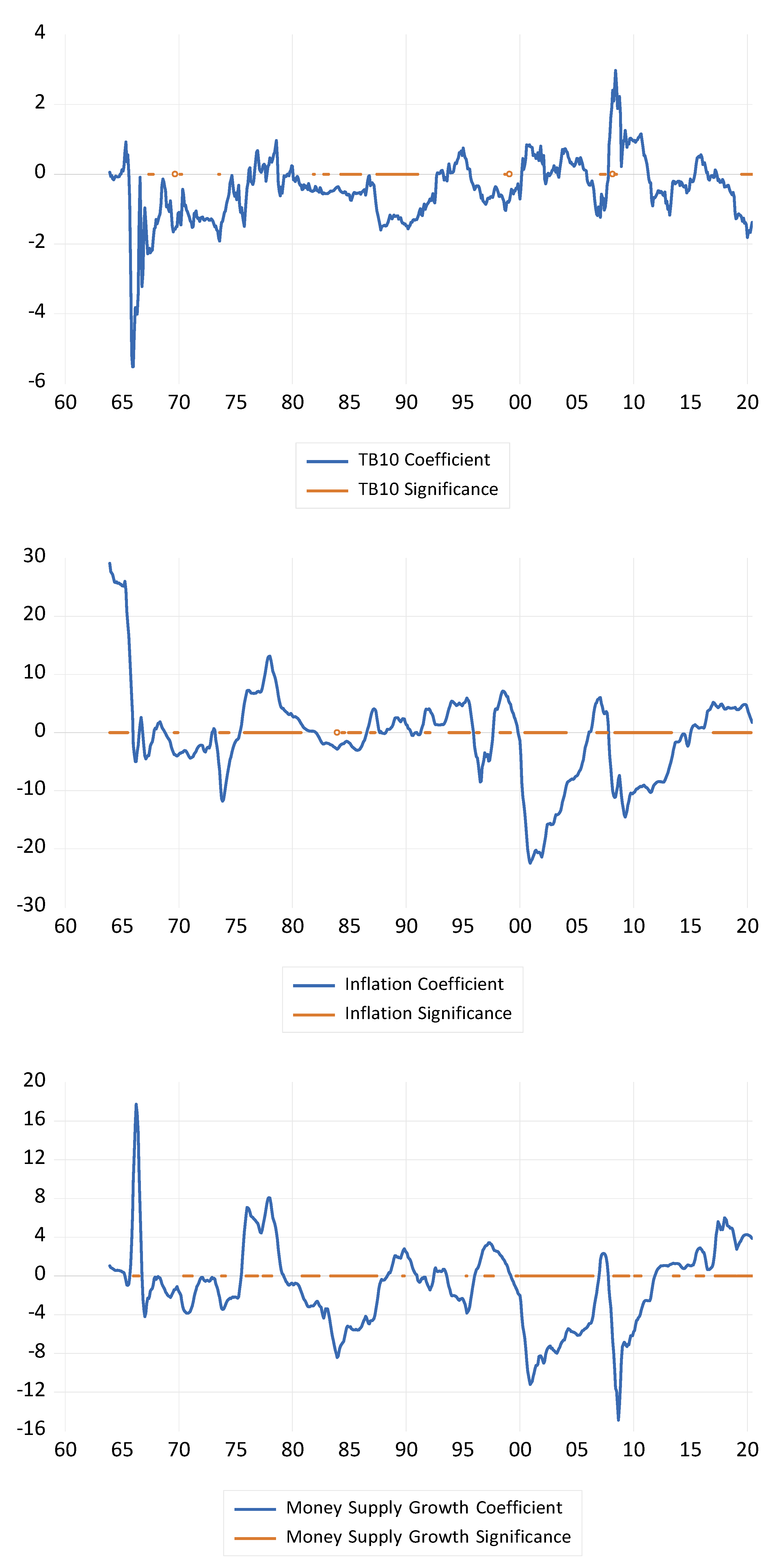
To further examine time-variation in the predictive regression, we consider a rolling regression approach. Figure 3 presents the rolling coefficients based on estimating Equation (3) over a 5-year window. In addition to the rolling coefficients, we highlight periods of statistical significance as indicated by the broken horizontal line. This line notes when the rolling coefficient is statistically significant (a t-statistic greater than 1.96 in absolute value), while gaps in the line indicate insignificance.14
For the rolling change in TB10 coefficient, we can observe that for the majority of the sample, the coefficient is negative, with only temporary periods of being positive. However, equally, the coefficient is mostly statistically insignificant, with the only prolonged period of significance arising during the 1980s and into the early 1990s. Positive values of the coefficient are typically associated with post-crisis periods, including the oil price shock of the mid-1970s, the early 1990s recession, the dotcom crash and financial crisis. Of note, the predictive coefficient becomes significantly negative at the end of the sample period.
The rolling predictive coefficients for inflation and money supply growth exhibit a similar pattern. This differs from the correlation analysis, in which the correlations involving TB10 and inflation are similar, while that involving money supply growth appears to mirror. Here, the inflation and money supply growth predictive coefficients follow a similar pattern, and the change in TB10 mirrors. Moreover, the coefficients for inflation and money supply growth are predominantly statistically significant. For both inflation and money supply growth coefficients, they are noticeably positive during the second half of the 1970s and 1990s, the mid-2000s and prior to the financial crisis and from the mid-2010s onwards. The coefficients are more noticeably negative during the early to mid-1980s (especially for money supply growth), the early 2000s and after the financial crisis.
For all three coefficients, the predictive relation is more likely to be negative than positive (the median value of each rolling coefficient is negative). Equally, after a crisis, the coefficients typically turn positive. However, there is a noticeable difference between the coefficient for the change in TB10, on the one hand, and the coefficients for inflation and money supply growth, on the other hand, after 2000. While the coefficient on TB10 is positive after the dotcom crash and financial crisis, the opposite is true for inflation and money supply growth. This suggests a change in the risk perception of these variables, with higher inflation and money supply now associated with lower risk. Moreover, there appears to be permanent shift in the inflation and money supply growth coefficients. While the change on TB10 coefficient again becomes negative post-crisis, for inflation and money supply growth, they switch to positive. This suggests that higher values of these variables indicate improving economic conditions and subsequently higher cashflows.
5. Summary and Conclusions
This paper examines the changing relation between stock returns and the three monetary variables of the long-term Treasury bond interest rates (TB10), inflation and money supply growth. Existing empirical evidence suggests a change in the stock return and bond relation; we thus extend this to consider further variables. Moreover, we look to explain the changing nature of the relations and, in particular, the role of risk.
We begin by examining the correlation between stock returns and the 10-Year Treasury bond yield (TB10), inflation and M2 money supply growth. Using both monthly and annualised data over the period from 1959 to mid-2020, we estimate the correlation coefficient over 5-year windows. Our results reveal that the correlation between stock returns and TB10 and inflation are predominately negative from the start of the sample but become increasingly positive following the dotcom crash and, especially, the financial crisis. The correlation between stock returns and money supply growth follows the opposite pattern, predominantly positive prior to 2000 and predominantly negative afterwards. Moreover, shifts in correlations appear to take place around periods of economic crisis.
To consider this further, we undertook two exercises modelling the correlation against variables that are identified in the literature as proxying for risk. A regression model for the change in correlation identifies real interest rates as the main determinant, along with output growth and the change in the dividend/price ratio. A probit regression using an indicator variable for the sign of the correlation highlights output growth, inflation and macroeconomic uncertainty as the main determinants, together with the change in the dividend/price ratio to a lesser extent. Each of these explanatory variables are linked to changing risk and support the view that correlations change in response to risk. For example, the switch to a positive correlation between stock returns and TB10 and inflation and the switch to a negative correlation between stock returns and money supply growth occurs with a decrease in output growth and an increase in macroeconomic uncertainty.
Building upon this analysis, we also consider the ability of each variable to predict stock returns and again consider the potential for time-variation. The results here also support a change in the nature of the relations. Again, the predictive regression allows us to consider how risk associated with these variables affects stock returns. Standard regression analysis suggests a negative predictive relation arising from all three variables for stock returns. The negative relations would indicate that a rise in each variable is associated with a decrease in the risk premium over the subsequent month, while an alternative, cashflow view would indicate that an increase in the predictor variables signals lower expected future cashflow.
However, both breakpoint and rolling regressions suggest that the relations are more involved. Notably, while a negative predictive relation does dominate through the sample period, it is punctuated by a change in the sign and associated with crisis periods. Thus, during these periods, an increase in these variables is associated with a higher risk premium. Moreover, from the dotcom crash period, there is a change in the behaviour of the predictive coefficient for TB10, on the one hand, and for both inflation and money supply growth, on the other. Notably, while a crisis continues to result in a positive coefficient for TB10, it now drives the coefficient on inflation and money supply growth to be more negative. This suggests a change in the perception of risk for risking inflation and money supply, where higher values now signal a lower risk premium and lower stock returns. In a period that is marked by historically low interest rates and inflation, arguably investors perceive the greater risk to be falls in inflation and money supply rather than increases. Equally, higher inflation and money supply growth signal improving future economic conditions and higher cashflows.
The results here suggest that each of the three monetary variables exhibit a relation, both contemporaneously and predictively, with stock returns. Of key importance, the nature of that relation has changed, most notably from the financial crisis but also after other crisis episodes. The results support the view that the effect of each variable on the risk premium switches sign after a crisis. Moreover, while such a switch is typically temporary, for both inflation and money supply growth, this effect remains after the financial crisis and may indicate a more permanent shift. This shifting nature of the risk premium between stocks and the variables included here is of importance to both academics involved in modelling the relations between financial variables and market participants in building investment strategies, and notably how changes in macroeconomic conditions affect their stock investments. As interest rates begin to rise in the post-pandemic period, it will be important for investors to consider a further switch in the nature of these relations.
Funding
The research received no external funding.
Institutional Review Board Statement
Not applicable.
Informed Consent Statement
Not applicable.
Conflicts of Interest
The authors declare no conflict of interest.
| 1 | Greater evidence of a positive stock return and inflation relation is noted at longer horizons (e.g., Engsted and Tanggaard 2002; Solnik and Solnik 1997). |
| 2 | Examples of previous research, which includes Homa and Jaffee (1971), Rogalski and Vinso (1977), Thorbecke (1997), Flannery and Protopapadakis (2002) and Chen (2009), report evidence of both a positive and negative relation. |
| 3 | The interested reader is directed towards Campbell and Shiller (1988) for greater details on the approach. In short, the expression is non-linear, and the Taylor approximation takes place around the dividend yield. The linearisation parameter is also defined therein. |
| 4 | The lowercase p and d now define the log values of P and D. |
| 5 | As noted, for the stock return and bond yield correlation examined here, the signs would be reversed with a positive correlation occurring in times of economic stress. |
| 6 | This includes evidence of a positive and negative relation as well as the potential for no relation. See, for example, Homa and Jaffee (1971), Kraft and Kraft (1977) Rogalski and Vinso (1977), Sorensen (1982), Thorbecke (1997), Flannery and Protopapadakis (2002) and Chen (2009). |
| 7 | We use industrial production and as a measure of growth consider both the first difference and the output gap from a Hodrick–Prescott trend. |
| 8 | We include inflation in all correlation regression. We also consider unexpected inflation as the residual from an AR(1) model for inflation. |
| 9 | We use the uncertainty measures of Jurado et al. (2015). |
| 10 | We use the national financial conditions index from the Chicago Federal Reserve. |
| 11 | High inflation will elicit a policy response (higher interest rates) that will lead to a subsequent economic downturn. However, (very) low inflation (or deflation) equally poses an economic risk in which firms and households may delay activity. |
| 12 | This also leads into a bigger discussion around the behaviour of stock prices including momentum effects and the disparity between price and value (e.g., Appel et al. 2012) and rationality (e.g., Schädler 2018). |
| 13 | The break in the 1980s occurs later than reported in the individual regressions. This may arise due to the nature of the tests where (approximately) 10 years of observations are required between each break. |
| 14 | Strictly speaking, these results are based on marginal significance and the potential exists that global significance is overstated (see, for example, Inoue and Rossi 2005). However, the illustrative nature of the results remains. |
References
- Alagidede, Paul, and Theodore Panagiotidis. 2012. Stock returns and inflation: Evidence from quantile regressions. Economics Letters 117: 283–86. [Google Scholar] [CrossRef] [Green Version]
- Andersson, Magnus, Elizaveta Krylova, and Sami Vähämaa. 2008. Why does the correlation between stock and bond returns vary over time? Applied Financial Economics 18: 139–51. [Google Scholar] [CrossRef]
- Appel, Dominik, Katrin Dziergwa, and Michael Grabinski. 2012. Momentum and reversal: An alternative explanation by non-conserved quantities. International Journal of Latest Trends in Finance and Economic Sciences 2: 8–16. [Google Scholar]
- Aslanidis, Nektarios, and Charlotte Christiansen. 2012. Smooth transition patterns in the realized stock-bond correlation. Journal of Empirical Finance 19: 454–64. [Google Scholar] [CrossRef]
- Aslanidis, Nektarios, and Charlotte Christiansen. 2014. Quantiles of the realized stock-bond correlation and links to the macroeconomy. Journal of Empirical Finance 28: 321–31. [Google Scholar] [CrossRef]
- Aslanidis, Nektarios, Charlotte Christiansen, and Andrea Cipollini. 2019. Predicting bonds betas using macro-finance variables. Finance Research Letters 29: 193–99. [Google Scholar] [CrossRef] [Green Version]
- Baele, Lieven, Geert Bekaert, and Koen Inghelbrecht. 2010. The determinants of stock and bond return comovements. Review of Financial Studies 23: 2374–428. [Google Scholar] [CrossRef]
- Bai, Jushan, and Pierre Perron. 1998. Estimating and testing linear models with multiple structural changes. Econometrica 66: 47–78. [Google Scholar] [CrossRef]
- Bai, Jushan, and Pierre Perron. 2003a. Computation and analysis of multiple structural change models. Journal of Applied Econometrics 18: 1–22. [Google Scholar] [CrossRef] [Green Version]
- Bai, Jushan, and Pierre Perron. 2003b. Critical values for multiple structural change tests. Econometrics Journal 6: 72–78. [Google Scholar] [CrossRef]
- Bali, Turan G., K. Ozgur Demirtas, and Hassan Tehranian. 2008. Aggregate earnings, firm-level earnings, and expected stock returns. Journal of Financial and Quantitative Analysis 43: 657–84. [Google Scholar] [CrossRef] [Green Version]
- Barnes, Michelle L. 1999. Inflation and returns revisited: A TAR approach. Journal of Multinational Financial Management 9: 233–45. [Google Scholar] [CrossRef]
- Barsky, Robert. 1989. Why don’t the prices of stocks and bonds move together? American Economic Review 79: 1132–45. [Google Scholar]
- Bernanke, Ben S., and Kenneth N. Kuttner. 2005. What explains the stock market’s reaction to Federal Reserve policy? Journal of Finance 60: 1221–57. [Google Scholar] [CrossRef] [Green Version]
- Bodie, Zvi. 1976. Common stocks as a hedge against inflation. Journal of Finance 31: 459–70. [Google Scholar] [CrossRef]
- Boudoukh, Jacob, and Matthew Richardson. 1993. Stock returns and inflation: A long-horizon perspective. American Economic Review 83: 1346–55. [Google Scholar]
- Campbell, John Y., and John Ammer. 1993. What moves the stock and bond markets? A variance decomposition for long-term asset returns. Journal of Finance 48: 3–37. [Google Scholar] [CrossRef]
- Campbell, John Y., and Robert J. Shiller. 1988. The dividend/price ratio and expectations of future dividends and discount factors. Review of Financial Studies 1: 195–228. [Google Scholar] [CrossRef] [Green Version]
- Chen, Shiu Sheng. 2009. Predicting the bear stock market: Macroeconomic variables as leading indicators. Journal of Banking and Finance 33: 211–23. [Google Scholar] [CrossRef]
- Connolly, Robert, Chris Stivers, and Licheng Sun. 2005. Stock market uncertainty and the stock-bond return relation. Journal of Financial and Quantitative Analysis 40: 161–94. [Google Scholar] [CrossRef] [Green Version]
- Connolly, Robert, Chris Stivers, and Licheng Sun. 2007. Commonality in the time variation of stock-bond and stock-stock return comovements. Journal of Financial Markets 10: 192–218. [Google Scholar] [CrossRef]
- Cornell, Bradford. 1983. Money supply announcements, interest rates and foreign exchange. Journal of International Money and Finance 1: 201–8. [Google Scholar] [CrossRef]
- Engsted, Tom, and Carsten Tanggaard. 2002. The relation between asset returns and inflation at short and long horizons. Journal of International Financial Markets, Institutions and Money 12: 101–18. [Google Scholar] [CrossRef]
- Fama, Eugene. 1981. Stock returns, real activity, inflation and money. American Economic Review 71: 545–65. [Google Scholar]
- Fama, Eugene F., and G. William Schwert. 1977. Asset returns and inflation. Journal of Financial Economics 5: 115–46. [Google Scholar] [CrossRef]
- Fan, Jack, and Marci Mitchell. 2017. Equity-Bond Correlation: A Historical Perspective. Graeme Capital Management Research Note. Rowayton: Graeme Capital Management, pp. 1–3. [Google Scholar]
- Fisher, Irving. 1930. The Theory of Interest. New York: Macmillan. [Google Scholar]
- Flannery, Mark J., and Aris A. Protopapadakis. 2002. Macroeconomic factors do influence aggregate stock returns. Review of Financial Studies 15: 751–82. [Google Scholar] [CrossRef]
- Friedman, Milton. 1961. The lag in effect of monetary policy. Journal of Political Economy 69: 447–66. [Google Scholar] [CrossRef]
- Gertler, Mark, and Peter Karadi. 2015. Monetary Policy Surprises, Credit Costs and Economic Activity. American Economic Review: Macroeconomics 7: 44–76. [Google Scholar]
- Geske, Robert, and Richard Roll. 1983. The fiscal and monetary linkage between stock returns and inflation. Journal of Finance 38: 1–33. [Google Scholar] [CrossRef]
- Gregoriou, Andros, Alexandros Kontonikas, Ronald MacDonald, and Alberto Montagnoli. 2009. Monetary policy shocks and stock returns: Evidence from the British market. Financial Markets and Portfolio Management 23: 401–10. [Google Scholar] [CrossRef]
- Gulko, Les. 2002. Decoupling. Journal of Portfolio Management 28: 59–66. [Google Scholar] [CrossRef]
- Hanson, Samuel G., and Jeremy C. Stein. 2015. Monetary Policy and Long-Term Real Rates. Journal of Financial Economics 115: 429–448. [Google Scholar] [CrossRef] [Green Version]
- Homa, Kenneth E., and Dwight M. Jaffee. 1971. The supply of money and common stock prices. Journal of Finance 26: 1045–66. [Google Scholar] [CrossRef]
- Inoue, Atsushi, and Barbara Rossi. 2005. Recursive predictability tests for real-time data. Journal of Business and Economic Statistics 23: 336–45. [Google Scholar] [CrossRef] [Green Version]
- Jurado, Kyle, Sydney C. Ludvigson, and Serena Ng. 2015. Measuring uncertainty. American Economic Review 105: 1177–216. [Google Scholar] [CrossRef]
- Kaul, Gautam. 1987. Stock returns and inflation: The role of the monetary sector. Journal of Financial Economics 18: 253–76. [Google Scholar] [CrossRef] [Green Version]
- Kraft, John, and Arthur Kraft. 1977. Determinants of common stock prices: A time series analysis. Journal of Finance 32: 417–25. [Google Scholar] [CrossRef]
- Lamont, Owen. 1998. Earnings and expected returns. Journal of Finance 53: 1563–87. [Google Scholar] [CrossRef]
- Li, Lingfeng. 2002. Macroeconomic Factors and the Correlation of Stock and Bond Returns. Yale International Center for Finance Working Paper, No 02-46. Available online: https://ssrn.com/abstract=363641 (accessed on 27 October 2021).
- Madadpour, Somayeh, and Mohsen Asgari. 2019. The puzzling relationship between stock returns and inflation: A review article. International Review of Economics 66: 115–45. [Google Scholar] [CrossRef]
- McMillan, David G. 2017. Does Money Supply Growth Contain Predictive Power for Stock Returns? Evidence and Explanation. International Journal of Banking, Accounting and Finance 8: 119–45. [Google Scholar] [CrossRef]
- Rankin, Ewan, and Muhummed Shah Idil. 2014. A Century of Stock-Bond Correlations. Sydney: Reserve Bank of Australia Bulletin, pp. 67–74. [Google Scholar]
- Rogalski, Richard J., and Joseph D. Vinso. 1977. Stock returns, money supply and the direction of causality. Journal of Finance 32: 1017–30. [Google Scholar] [CrossRef]
- Schädler, Tobias. 2018. Measuring Irrationality in Financial Markets. Archives of Business Research 6: 252–59. [Google Scholar]
- Schädler, Tobias, and Michael Grabinski. 2015. Income from Speculative Financial Transactions will always Lead to Macro-Economic Instability. International Journal of Finance, Insurance and Risk Management 5: 922–32. [Google Scholar]
- Sellin, Peter. 2001. Monetary policy and the stock market: Theory and Empirical Evidence. Journal of Economic Surveys 15: 491–541. [Google Scholar] [CrossRef]
- Shiller, Robert J., and Andrea E. Beltratti. 1992. Stock prices and bond yields: Can their comovements be explained in terms of present value models? Journal of Monetary Economics 30: 25–46. [Google Scholar] [CrossRef]
- Schotman, Peter C., and Mark Schweitzer. 2000. Horizon sensitivity of the inflation hedge of stocks. Journal of Empirical Finance 7: 301–15. [Google Scholar] [CrossRef]
- Söderlind, Paul. 1998. Nominal Interest Rates as Indicators of Inflation Expectations. Scandinavian Journal of Economics 100: 457–472. [Google Scholar] [CrossRef]
- Solnik, Bruno, and Vincent Solnik. 1997. A multi-country test of the Fisher model for stock returns. Journal of International Financial Markets, Institutions and Money 7: 289–301. [Google Scholar] [CrossRef]
- Sorensen, Eric H. 1982. Rational expectations and the impact of money upon stock prices. Journal of Financial and Quantitative Analysis 17: 649–62. [Google Scholar] [CrossRef]
- Stulz, Rene M. 1986. Asset pricing and expected inflation. Journal of Finance 41: 209–23. [Google Scholar] [CrossRef]
- Thorbecke, Willem. 1997. On stock market returns and monetary policy. Journal of Finance 52: 635–54. [Google Scholar] [CrossRef]
- Viceira, Luis M. 2012. Bond risk, bond return volatility, and the term structure of interest rates. International Journal of Forecasting 28: 97–117. [Google Scholar] [CrossRef]
Figure 1.
Time series data plots.

Figure 2.
5-year rolling correlations.

Figure 3.
Rolling predictive coefficients and significance.


Table 1.
Summary statistics.
| Mean | Med | Min | Max | SD | Skew | Kurt | JB—p | |
|---|---|---|---|---|---|---|---|---|
| Monthly Data | ||||||||
| SR | 0.550 | 0.924 | −22.805 | 11.352 | 3.606 | −1.213 | 8.191 | 0.00 |
| TB10 (/12) | 0.498 | 0.474 | 0.055 | 1.277 | 0.240 | 0.769 | 3.394 | 0.00 |
| Inflation | 0.296 | 0.253 | −1.786 | 1.794 | 0.313 | 0.256 | 7.511 | 0.00 |
| M2 | 0.563 | 0.528 | −0.561 | 6.452 | 0.454 | 4.983 | 55.601 | 0.00 |
| Annualised Data | ||||||||
| SR | 6.548 | 9.195 | −55.353 | 42.298 | 15.179 | −0.970 | 4.531 | 0.00 |
| TB10 | 5.980 | 5.690 | 0.660 | 15.32 | 2.884 | 0.769 | 3.394 | 0.00 |
| Inflation | 3.599 | 2.921 | −1.978 | 13.621 | 2.672 | 1.516 | 5.351 | 0.00 |
| M2 | 6.578 | 6.527 | 0.229 | 20.809 | 2.706 | 0.343 | 4.006 | 0.00 |
| Correlations | ||||||||
| SR | TB10 | Inflation | M2 | |||||
| SR | 1 | −0.015 | −0.043 | −0.049 | ||||
| TB10 | 0.019 | 1 | 0.466 | 0.003 | ||||
| Inflation | −0.154 | 0.676 | 1 | −0.095 | ||||
| M2 | 0.012 | 0.177 | 0.156 | 1 | ||||
Notes: SR is stock returns as the log difference of the index, TB10 is the 10-Year Treasury bond yield, Inflation is the log difference of CPI, M2 is the growth rate, log difference, of M2 money supply, all measured over both monthly (one-period) and annual (12-period) horizons. For the correlations, the bottom-left triangle refers to the annual data, and the top-right triangle refers to the monthly data.
Table 2.
Correlation regressions.
| Δ in Correlation Regression | ||||||
|---|---|---|---|---|---|---|
| ΔReal IR | IP Growth | Inflation | ΔDP | Uncertainty | NFCI | |
| SR-TB10 | 0.007 (2.41) | −0.128 (−2.36) | 0.208 (1.61) | 0.081 (2.30) | 0.010 (0.21) | −0.008 (−2.44) |
| SR-Inflation | 0.010 (2.05) | −0.123 (−2.11) | −0.084 (−0.35) | 0.094 (1.99) | 0.031 (0.43) | 0.005 (1.08) |
| SR-M2 | −0.007 (−2.11) | −0.040 (−0.80) | −0.007 (−0.06) | −0.069 (−1.24) | −0.116 (−2.24) | −0.001 (−0.37) |
| Probit Correlation Sign Regression | ||||||
| SR-TB10 | −0.039 (−0.29) | −0.437 (−2.56) | −0.159 (−4.98) | 0.140 (2.83) | 0.719 (5.94) | −0.047 (−0.48) |
| SR-Inflation | 0.059 (0.47) | −0.286 (−1.86) | −0.136 (−4.67) | −0.429 (0.85) | 0.431 (4.03) | −0.089 (−0.89) |
| SR-M2 | 0.135 (0.88) | 0.933 (4.45) | 0.523 (10.70) | −0.243 (−4.05) | −0.119 (−7.81) | 0.149 (1.24) |
Notes: Entries are the coefficients (and t-statistics) based on Equation (4) for the change in the correlation and Equation (5) for the sign of the correlation. The first column is the correlation pairs, while the explanatory variables are the change in the real interest rate (ΔReal IR), the rate of growth in industrial production (IP), inflation, the change in the dividend/price ratio (ΔDP), macroeconomic uncertainty based on the measure of Jurado et al. (2015) and National Financial Conditions Index (NCFI) from the Chicago Federal Reserve.
Table 3.
Linear predictive regression results.
| Model | ΔTB10 | Inflation | M2 Growth |
|---|---|---|---|
| Monthly Data | |||
| 1 | −0.268 (−4.72) | - | - |
| 2 | - | −1.337 (−2.37) | - |
| 3 | - | - | 0.516 (1.35) |
| 4 | −0.237 (−4.00) | −1.631 (−1.63) | 0.384 (1.06) |
| Annualised Data | |||
| 1 | −0.070 (−3.10) | - | - |
| 2 | - | −0.459 (−0.91) | - |
| 3 | - | - | −0.947 (−2.54) |
| 4 | −0.061 (−2.60) | −0.250 (−0.49) | −0.855 (−2.25) |
Notes: Entries are the coefficients (and t-statistics) based on Equation (6) for stock returns with lags of the variables listed in the first row as predictors, both individually and jointly.
Table 4.
Predictive regression with breaks.
| ΔTB10 | |||||
| Date | 1959:01–1981:11 | 1981:12–1999:09 | 1999:10–2008:09 | 2008:10–2020:06 | |
| Coef (tstat) | −0.063 (−2.11) | −0.091 (−3.13) | 0.077 (0.91) | −0.039 (−1.00) | |
| Inflation | |||||
| Date | 1959:01–1972:10 | 1972:11–1981:10 | 1981:11–1999:10 | 1999:11–2009:05 | 2009:06–2020:06 |
| Coef (tstat) | −0.937 (−0.53) | 2.836 (3.26) | 0.523 (0.44) | −7.930 (−2.47) | 0.942 (0.81) |
| M2 Growth | |||||
| Date | 1959:01–2008:09 | 2008:10–2020:06 | |||
| Coef (tstat) | −1.168 (−2.92) | 1.834 (2.46) | |||
| Joint Regression | |||||
| Date | 1959:01–1974:07 | 1974:08–1986:10 | 1986:11–1999:10 | 1999:11–2008:09 | 2008:10–2020:06 |
| ΔTB10 | −0.103 (−1.39) | −0.052 (−2.77) | −0.075 (−1.79) | 0.087 (1.29) | −0.032 (−0.93) |
| Infl | −2.781 (−2.26) | −1.261 (−2.28) | −1.710 (−1.15) | −10.270 (−2.78) | −0.231 (−0.18) |
| M2 | −1.240 (−1.26) | −4.257 (−5.93) | −0.444 (−0.46) | −7.563 (−5.14) | 1.801 (2.49) |
Notes: Entries are the coefficients (and t-statistics) based on Equation (6) for stock returns with lags of each variable estimated using the Bai–Perron breakpoint approach. Regressions are conducted for each individual predictor variable as well as jointly.
Publisher’s Note: MDPI stays neutral with regard to jurisdictional claims in published maps and institutional affiliations. |
© 2021 by the author. Licensee MDPI, Basel, Switzerland. This article is an open access article distributed under the terms and conditions of the Creative Commons Attribution (CC BY) license (https://creativecommons.org/licenses/by/4.0/).
Share and Cite
MDPI and ACS Style
McMillan, D.G. The Time-Varying Relation between Stock Returns and Monetary Variables. J. Risk Financial Manag. 2022, 15, 9. https://0-doi-org.brum.beds.ac.uk/10.3390/jrfm15010009
AMA Style
McMillan DG. The Time-Varying Relation between Stock Returns and Monetary Variables. Journal of Risk and Financial Management. 2022; 15(1):9. https://0-doi-org.brum.beds.ac.uk/10.3390/jrfm15010009
Chicago/Turabian StyleMcMillan, David G. 2022. "The Time-Varying Relation between Stock Returns and Monetary Variables" Journal of Risk and Financial Management 15, no. 1: 9. https://0-doi-org.brum.beds.ac.uk/10.3390/jrfm15010009