Probabilistic Forecasting Model of Solar Power Outputs Based on the Naïve Bayes Classifier and Kriging Models


Department of Electrical Engineering, Sangmyung University, Seoul 03016, Korea
*
Author to whom correspondence should be addressed.
Energies 2018, 11(11), 2982; https://0-doi-org.brum.beds.ac.uk/10.3390/en11112982
Submission received: 27 September 2018
/
Revised: 25 October 2018
/
Accepted: 30 October 2018
/
Published: 1 November 2018
(This article belongs to the Special Issue Data Science and Big Data in Energy Forecasting with Applications)
Abstract
:Solar power’s variability makes managing power system planning and operation difficult. Facilitating a high level of integration of solar power resources into a grid requires maintaining the fundamental power system so that it is stable when interconnected. Accurate and reliable forecasting helps to maintain the system safely given large-scale solar power resources; this paper therefore proposes a probabilistic forecasting approach to solar resources using the R statistics program, applying a hybrid model that considers spatio-temporal peculiarities. Information on how the weather varies at sites of interest is often unavailable, so we use a spatial modeling procedure called kriging to estimate precise data at the solar power plants. The kriging method implements interpolation with geographical property data. In this paper, we perform day-ahead forecasts of solar power based on the probability in one-hour intervals by using a Naïve Bayes Classifier model, which is a classification algorithm. We augment forecasting by taking into account the overall data distribution and applying the Gaussian probability distribution. To validate the proposed hybrid forecasting model, we perform a comparison of the proposed model with a persistence model using the normalized mean absolute error (NMAE). Furthermore, we use empirical data from South Korea’s meteorological towers (MET) to interpolate weather variables at points of interest.
1. Introduction
Solar energy utilization is rapidly growing all over the world. According to the International Renewable Energy Agency (IRENA), solar power generation capacity was 397 GW at the end of 2017. It took first place again with a capacity increase of 94 GW, accounting for a 32% increase—higher than the 10% wind power growth rate [1]. In the United States, the electric power company PJM will supply 13% of its total load as renewable energy by 2031. In the case of solar power generation, installed capacity will be increased to 8.1 GW by 2027 [2]. South Korea’s solar power generation capacity is 904.1 MW and its cumulative installation capacity is 4519.4 MW as of 2016, which is a small percentage compared with existing generators. As solar power generation capacity increases, many electric utilities are expected to have difficulty managing power system planning and operation. Meteorological variables that change over time and space mean that solar energy is highly intermittent and uncertain. Forecasting among various technologies can play an important role in preventing transmission congestion and maintaining a power balance, thus reducing the difficulty. Various forecasting techniques are being formulated abroad. UC San Diego uses a Total Sky Imager to predict the movement and location of clouds to forecast solar irradiation levels, determines the sky cover every 30 s, and estimates the position of clouds 5 min in advance [3,4]. San Antonio, Texas, U.S. uses satellites to forecast and assess solar irradiation for use in solar power systems and power system planning and integration [5]. In addition, a review of recent forecasting methods as related to solar generation resources is shown in [6,7]. Reference [6] accentuates the need for accurate forecasting of intermittent resources to achieve power gird balance. Various methods are currently being studied for the forecasting of solar energy resources, such as clear sky models, regressive methods, Artificial Intelligence (AI) techniques, remote sensing models, Numerical Weather Prediction (NWP), Local sensing, and Hybrid systems. In NWP-based forecast, reference [8] used the Environment Canadas Global Environmental Multiscale NWP model to forecast hourly Global Horizontal Irradiance (GHI) and solar power for horizons out to 48 h. They applied spatial averaging and bias removal using a Kalman filter on the NWP forecasts to increase the predictions’ accuracy. Reference [9] used NWP forecasts from the National Weather Service’s (NWS) database as exogenous inputs for Artificial Neural Networks (ANNs) to predict hourly GHI and Direct Normal Irradiance (DNI) out to 6 days ahead of time for Merced, California. In stochastic forecasts, reference [10] constructed three autoregressive integrated moving average (ARIMA) forecasting models for next-hour GHI including cloud cover effects. The main difference in the three models tested concerns the inputs used: GHI in the first model, DNI and Diffuse Horizontal Irradiance (DHI) in the second model, and cloud cover (CC) in the third model. The authors used the third typical meteorological year (TMY3) data from the National Solar Radiation Data Base [11] to estimate the ARIMA models and to validate the forecasting accuracy. In AI forecasting, reference [12] used an ANN with exogenous variables to forecast the hourly solar power for a forecasting horizon of 12 h. This model shows an improvement in root-mean-square error (RMSE) of about 2.07%. Reference [13] applied several stochastic and AI techniques (ARIMA, k-Nearest Neighbor (k-NN), ANN) to predict the one- and two-hour averaged power output of a 1 MW solar power plant in Merced, California. In hybrid forecasting, hybrid models have recently been used to improve forecast error by combining the benefits of forecasting models. Reference [14] tested hybrid forecasting models that combine information from processed satellite images with ANNs.
Many solar forecasting methods use expensive and restricted equipment, such as satellite images and sky imagers, and complex equations. In addition, existing forecasting methods take a deterministic approach that represents a single value for a forecasting target. This has limited ability to express uncertainty in solar energy [15,16,17,18]. Some recent works have dealt with probabilistic forecasting for addressing uncertainty in solar energy. References [19,20] assess the performance of three probabilistic models for intra-day solar forecasting. The results demonstrated that the NWP exogenous inputs improve the quality of the intra-day probabilistic forecasts. Reference [21] shows three different methods for ensemble probabilistic forecasting, derived from seven individual machine learning models, to generate 24-h-ahead solar power forecasts. The results have shown that the ensemble models offer even more accurate results than any individual machine learning model like ARIMA. GEFCOM represents a general framework of probabilistic forecasts for renewable energy generation [22,23]. This is demonstrated by an application in probabilistic solar power forecasting. The results from its evaluation show that the RMSE and quantile score are quite low, verifying the precision of the proposed forecasting method. This paper proposes a probabilistic approach for solar power forecasting using spatial interpolation and a naïve Bayes Classifier. Section 2 describes the hybrid forecasting model of solar energy resources using kriging and naïve Bayes Classifier models. First, we show the spatial interpolation using what is called the kriging method. This method can spatially estimate the weather factor at different points of interest using a current weather value without historical data. Next, we propose a method for solar power forecasting using a naïve Bayes Classifier. This method can probabilistically forecast solar power in one-hour intervals. Section 3 verifies the proposed method. We apply a hybrid spatio-temporal forecasting model that combines kriging and naïve Bayes Classifier based on empirical NWP data in South Korea. We also perform a comparison of the proposed model with a persistence model using normalized mean absolute error (NMAE) to validate the proposed hybrid forecasting model.
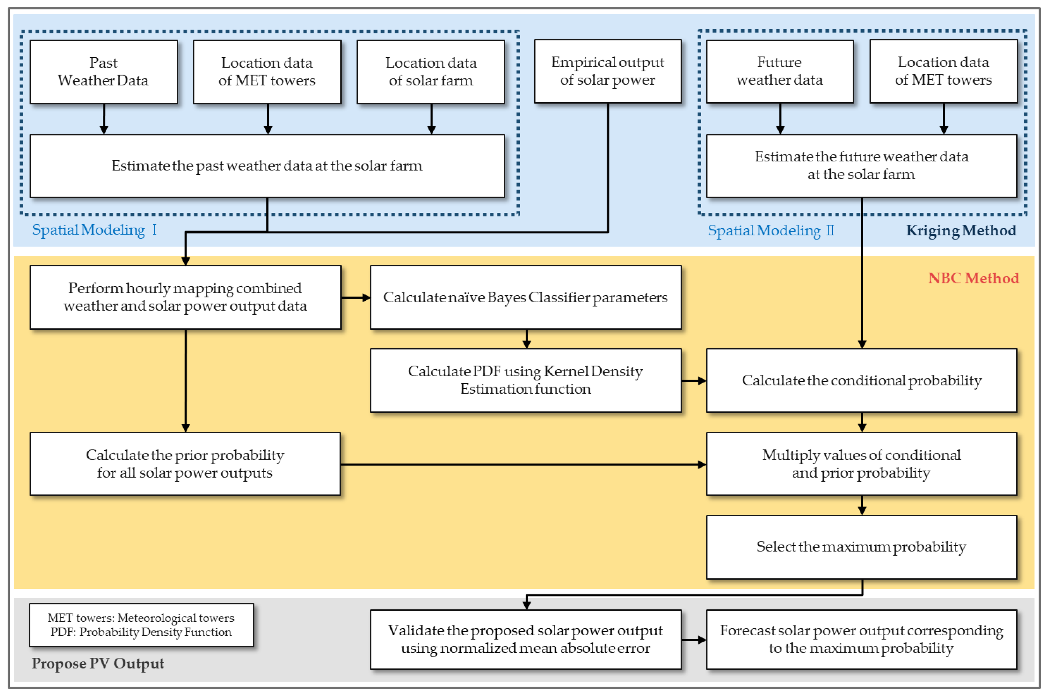
2. A Hybrid Spatio-Temporal Forecasting Model
We introduce a hybrid method to probabilistically forecast solar power output using kriging and a naïve Bayes Classifier. Weather factors and historical data of solar power have a significant impact on forecasting the amount of solar power [24,25]. However, obtaining data on meteorological variables that can change at any point of interest necessitates expensive equipment, and acquiring weather data over time and determining the forecast generation outputs based on that takes a long time. This paper estimates weather variables at points of interest economically and efficiently through a type of spatial modelling called kriging. In addition, solar power varies according to humidity, temperature, cloud cover amount, and wind speed; in particular, irradiation has the greatest influence on determining solar power output [26]. However, since they have high variability and uncertainty, it is essential to use a probabilistic method. Figure 1 below shows the algorithm for the hybrid forecasting model.
2.1. Spatial Modelling Using the Kriging Technique
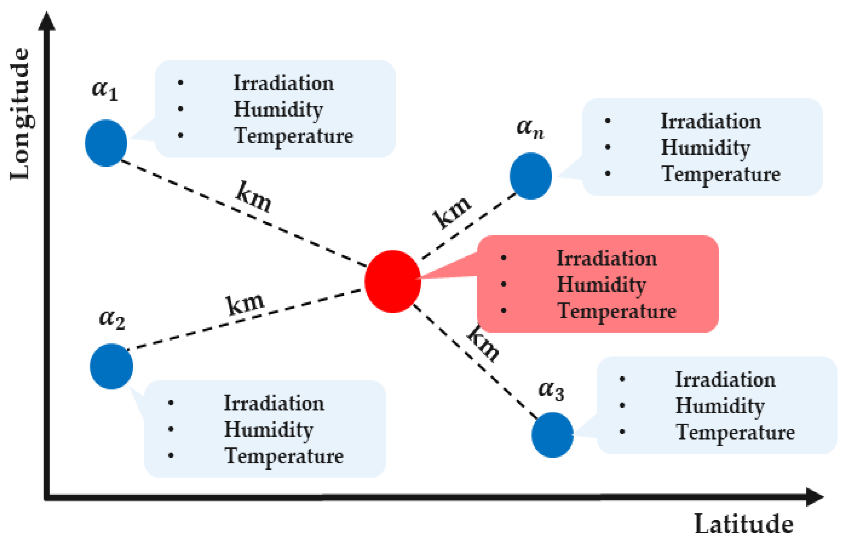
Spatial Modeling is a geo-statistics technique used in various fields of geoscience and engineering, such as pollution concentration and precipitation analysis, to analyze physical phenomena or data with spatial characteristics [27]. This allows values of interest to be estimated using only current values and location data without historical data. Kriging is one spatial interpolation method that estimates data at target points based on regression against observed values of neighbor points, weighted according to spatial covariance values. The general formula for the ordinary kriging method is as shown in Equation (1) [28]:
where is the estimated value of the target point, is a weight regarding the spatial distances between two points, and is the number of neighbor points. In the ordinary kriging method, the weight must sum to 1 to avoid biased models and thus minimize the error variance between estimated and actual values. This method can be represented as shown in Figure 2.
We minimize the error variance in the ordinary kriging method using the Lagrange function. is the objective function of the Lagrange and is the Lagrange factor as shown in Equation (2) [29].
Performing the kriging method requires the weights of the ambient points; these values are combined linearly to estimate the results of spatial modelling. This equation has a minimum value in extremum, so we must perform two partial differentiations for and as shown in Equations (3) and (4). After we have solved the above equation, can finally express the weights for neighboring points. However, as noted in Equation (1) [29], the sum of weights is 1.
2.2. Probabilistic Forecasting for Solar Power Using a Naïve Bayes Classifier
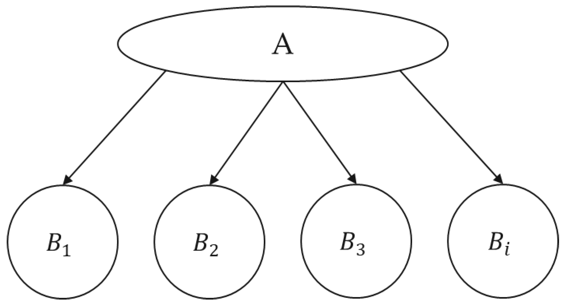
A Naïve Bayes Classifier is machine learning technique based on Bayes probabilistic theory that represents the relationship between a prior probability and posterior probability using conditional probabilities [30,31,32,33,34]; it deals with decision problems mathematically under uncertainty and creates a simple and efficient model in the field of document taxonomy and disease prediction [35,36]. This method makes classification rules based on historical data and applies new values to the class that is arranged according to predefined rules. The general formula for a Naïve Bayes Classifier is as shown in Equation (5) [30,31,32,33,34]:
where A and B are different events, A is a random variable denoting the class of an instance, and B is a vector of random variables denoting observed attribute values. This assumes that attribute values are independent, which means that one of several attribute values does not affect the other attribute values. When depicted graphically, a Naïve Bayes Classifier has a form such as that shown in Figure 3.
This assumption supports efficient algorithms that are simple to compute for test cases and to estimate from training data. The independency assumption means that the conditional probability is represented by the chain rule as shown in Equation (6) [30,31,32,33,34].
The probability of the attribute value located in the denominator serves as a normalized constant and does not affect the probability results, so we have omitted it for convenience of calculation. When we assign a new attribute value to a class based on predefined classification criteria, all classes will have a post probability, and the class among them with the maximum probability is finally selected as shown in Equation (7) [30,31,32,33,34].
A Naïve Bayes Classifier consists of prior and posterior probabilities. First, a “prior probability” is a probability that event A will occur before event B, and it gives the number of classes. refers to the ratio of the number of specific classes for all classes, . The prior probability is represented as shown in Equation (8) below. The larger the amount of data, the more different the class, and the prior probability can be adjusted depending on the class range setting [30,31,32,33,34].
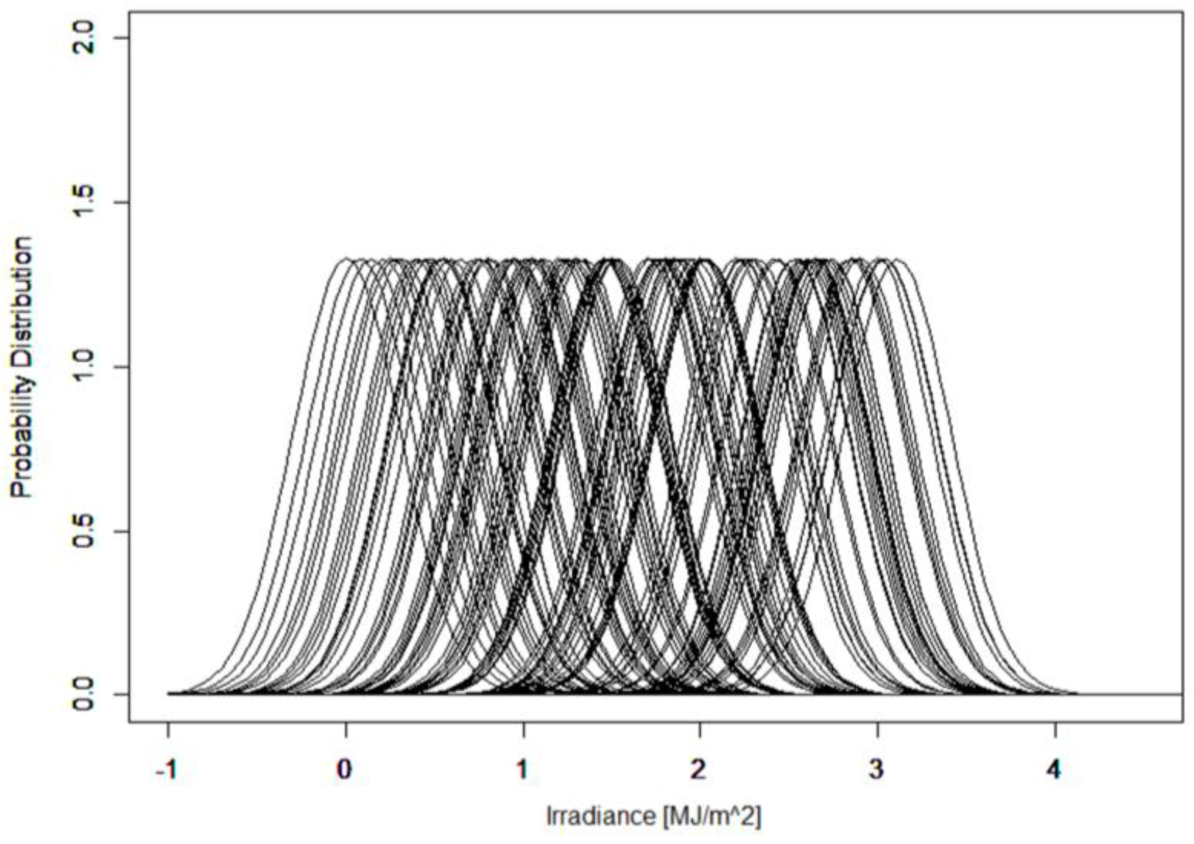
A “conditional probability” is the probability that event A will occur when event B happens. We calculated the probability for the occurrence of event A using a probability distribution because it is generally assumed to follow a normal distribution in the Naïve Bayes Classifier method. This is fulfilled by a graph in which the probability distribution is symmetrical in relation to the mean.
This is determined by the new value and the defined normal distribution. The Naïve Bayes Classifier treats discrete and numeric attributes somewhat differently. For each discrete attribute, the conditional probability is modeled as a single number between 0 and 1. In contrast, each numeric attribute is modeled by some continuous probability distribution over the range of that attribute’s values. We can write continuous attributes as shown in Equation (9) where is the new attribute’s value, is its mean, and is its standard deviation [30,34].
3. Experimental Study: Probabilistic Forecasting of Solar Power Outputs in South Korea
3.1. Estimating Weather Data at Solar Farm “A” Using the Kriging Technique
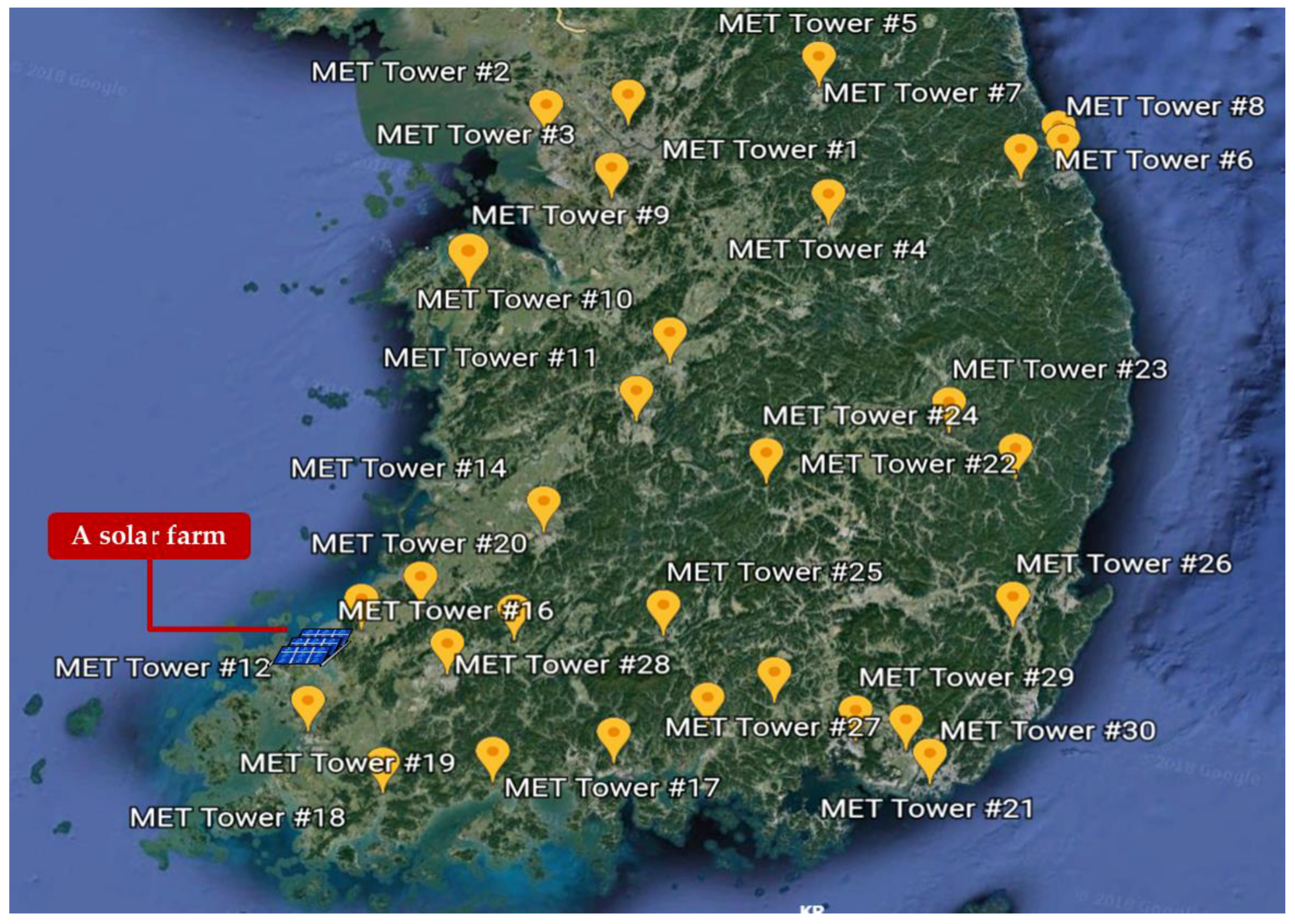
In this case study, we forecast the output of solar power a day ahead in South Korea. We applied the kriging technique using weather information and location data for neighbor points. Figure 4 represents solar farm site “A” and 30 nearby meteorological towers in South Korea using Google Maps. Before applying the kriging method, we collected latitude and longitude data for both the meteorological towers and solar farm “A”. Table 1 shows the coordinate data for applying the kriging method. The weather information was measured at the meteorological towers from 1 January 2015 to December 2016 in hourly intervals.
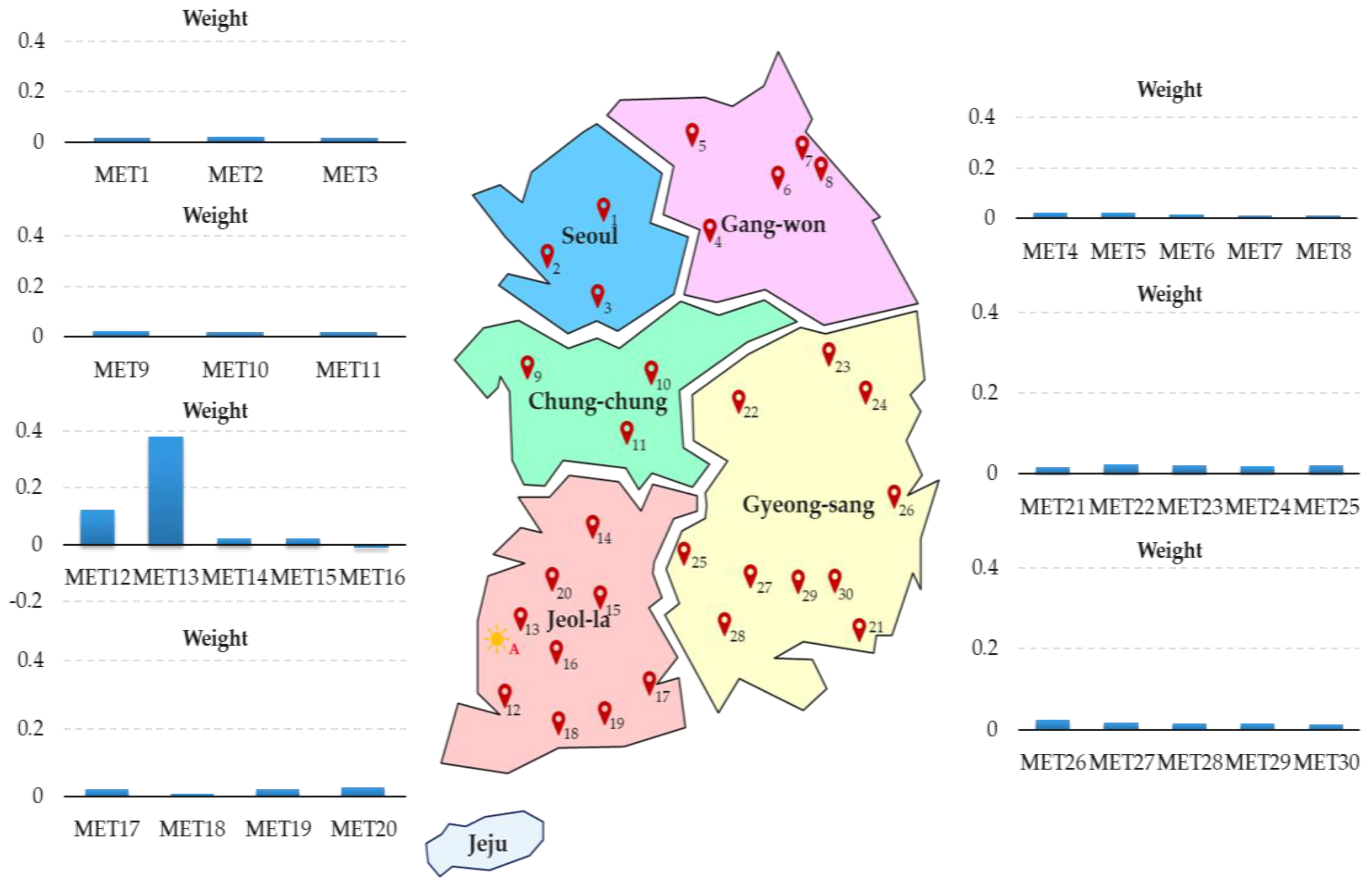
We estimated the weather data at the solar farm using information relating to neighboring points; we need the weights of 30 meteorological points for 1 site of interest. We calculated these weights based on the spatial correlation, and sum of the weights must be 1. Figure 5 shows the locations and weights of neighboring points. MET 13 has the greatest impact on the point of interest. Table 2 provides detailed weights of METs.
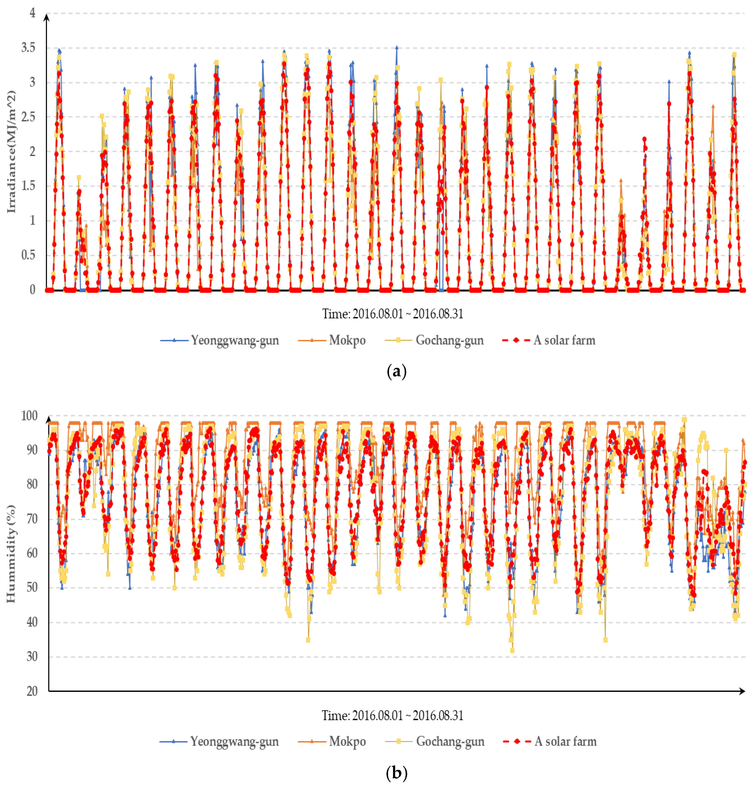
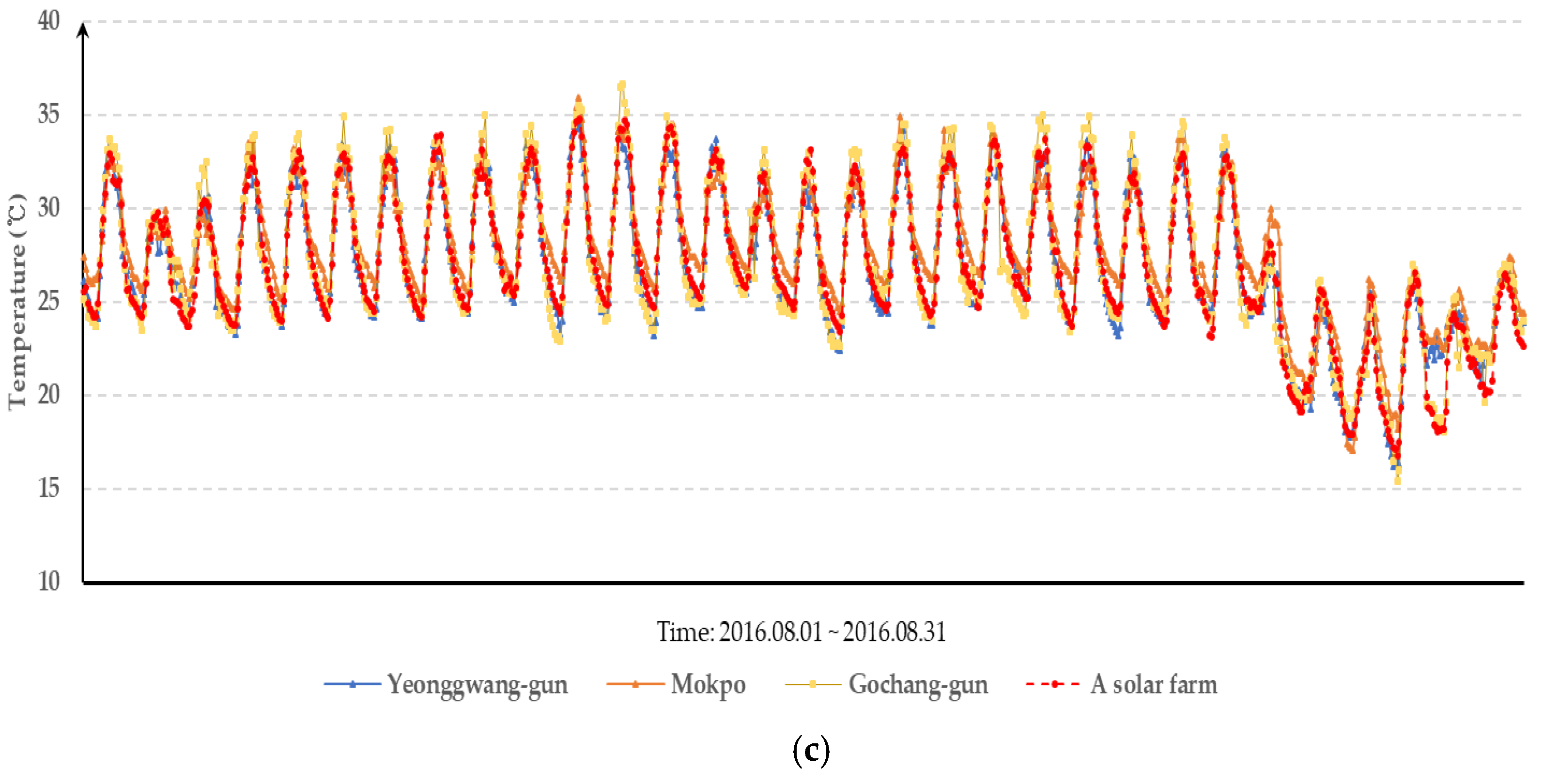
We performed the kriging method to estimate the weather information at the solar farm in 2016. The result of estimating the irradiance, humidity, and temperature linearly combine the weights and values of weather information for neighboring points using Equation (1). Figure 6 shows the results of the kriging method at solar farm “A” for August 2016.
To verify to the accuracy of the model, cross validation was performed. After assuming that the acquired meteorological data was unknown, we compared the actual and forecast data by the remaining data. Table 3 shows the results of cross validation of irradiance for five points representing each administrative district.
Now, we need to make a classifier for solar power output forecast using a Naïve Bayes Classifier based on a probabilistic approach. Therefore, we must map weather data and solar power output data by the hour.
3.2. Probabilistic Forecasting for Solar Power Using a Naïve Bayes Classifier Technique
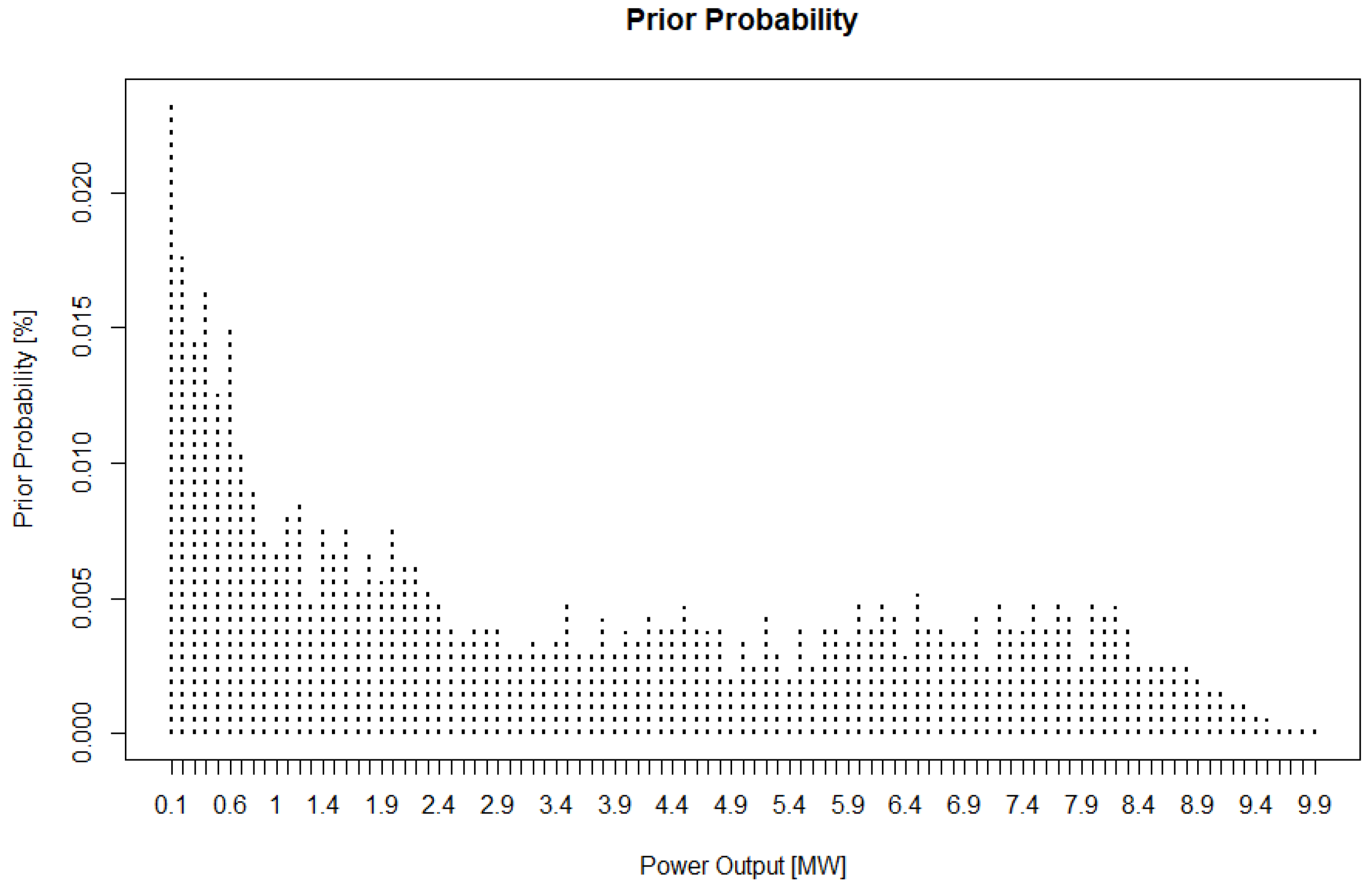
We forecasted the output of solar farm “A” based on the estimated weather data for 30 neighboring points. The prior and conditional probability are essential components of forecasting the solar power output. We calculated the prior probability for each solar power output at solar farm “A” using Equation (8); the results are as shown in Figure 7. In this figure, a value of 0 among the solar power output values was excluded because the prior probability corresponding to 0 was significantly higher than the other output values.
We used the prior probability calculated above to forecast the amount of solar power by multiplying it by the conditional probability. In addition, we could optionally utilize Laplacian correction to avoid the problem in which there is a 0 for the prior probability to produce outputs that do not exist in the past.
Finally, we must compute the conditional probability regarding each weather factor to forecast the solar power output since we treat numeric attributes over the range of an attribute’s values. Figure 8 shows the normal distribution of solar irradiance that could occur when the solar power output is 4.9 MW. In the event of 4.9 MW, it indicates that irradiance occurs in the middle.
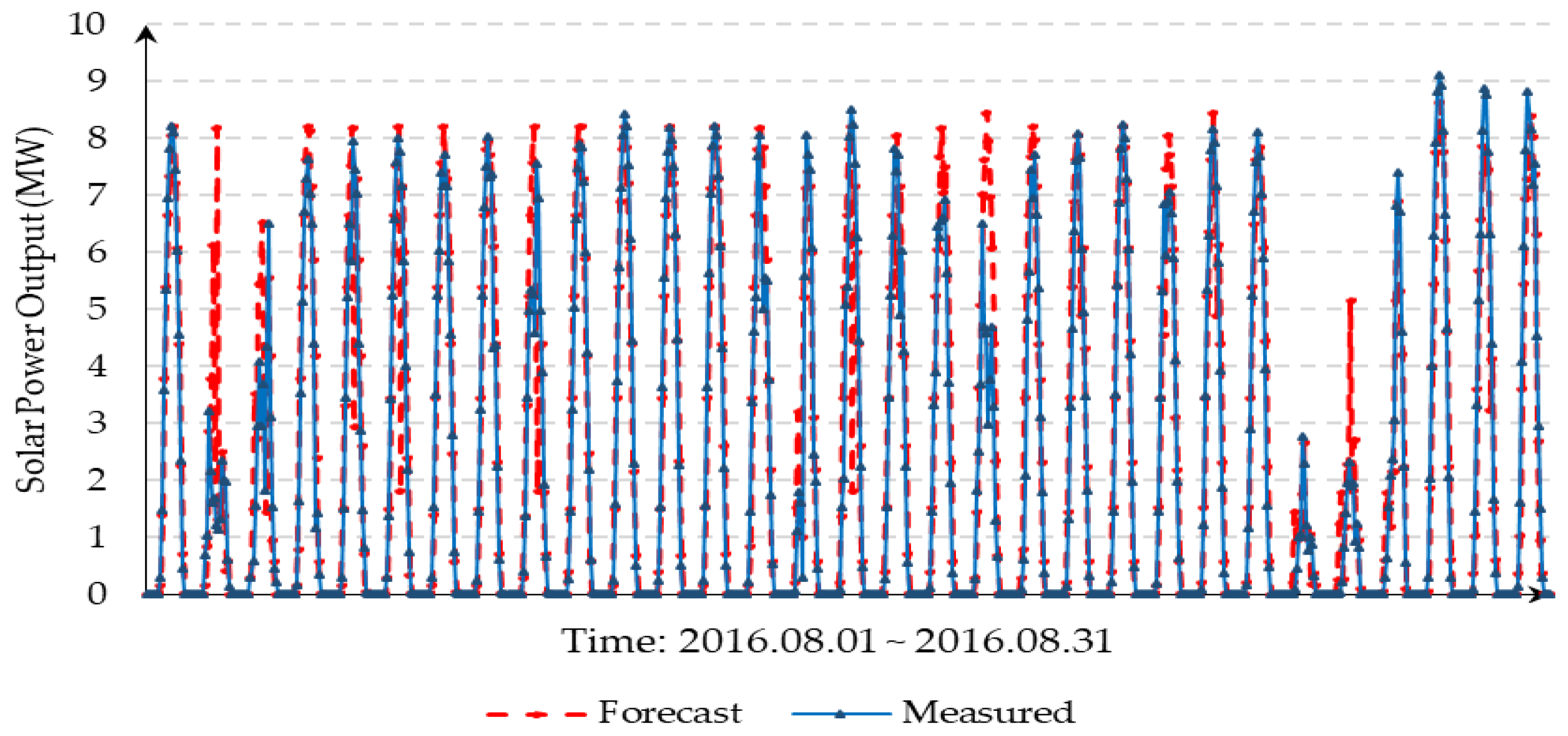
We calculated the probabilities of the estimated weather values, such as in Figure 6, at the solar farm by applying them at the forecast point to the predefined classifier. We classified all models according to the solar power output values provided with the estimated weather values and showed the probability through a continuous normal distribution function. The summation of the conditional probability and the prior probability as shown in Equation (6) allows us to determine the post probability for each model. We can acquire one model with the maximum probability as shown in Equation (7). Based on data from 2015 up to the previous day of forecasting, we can forecast the solar power output by selecting the models with highest probability for the year 2016. Figure 9 shows two outputs of solar power by comparing the actual and forecast values over August. The red line is the output value predicted by the Naïve Bayes Classifier technique, and the blue line is the actual output value measured at solar farm “A”.
We performed day-ahead forecasting for the year 2016 and we used the NMAE (%) to view the accuracy of the forecast using the Naïve Bayes Classifier method. Table 4 describes the NMAE for the results of each forecasting model, and expresses a percentage of the installed capacity, 11 MW. The NMAE is as shown in Equation (10) [37,38]:
where and are the actual and forecasted solar power for period h, and refers to the installed solar power capacity.
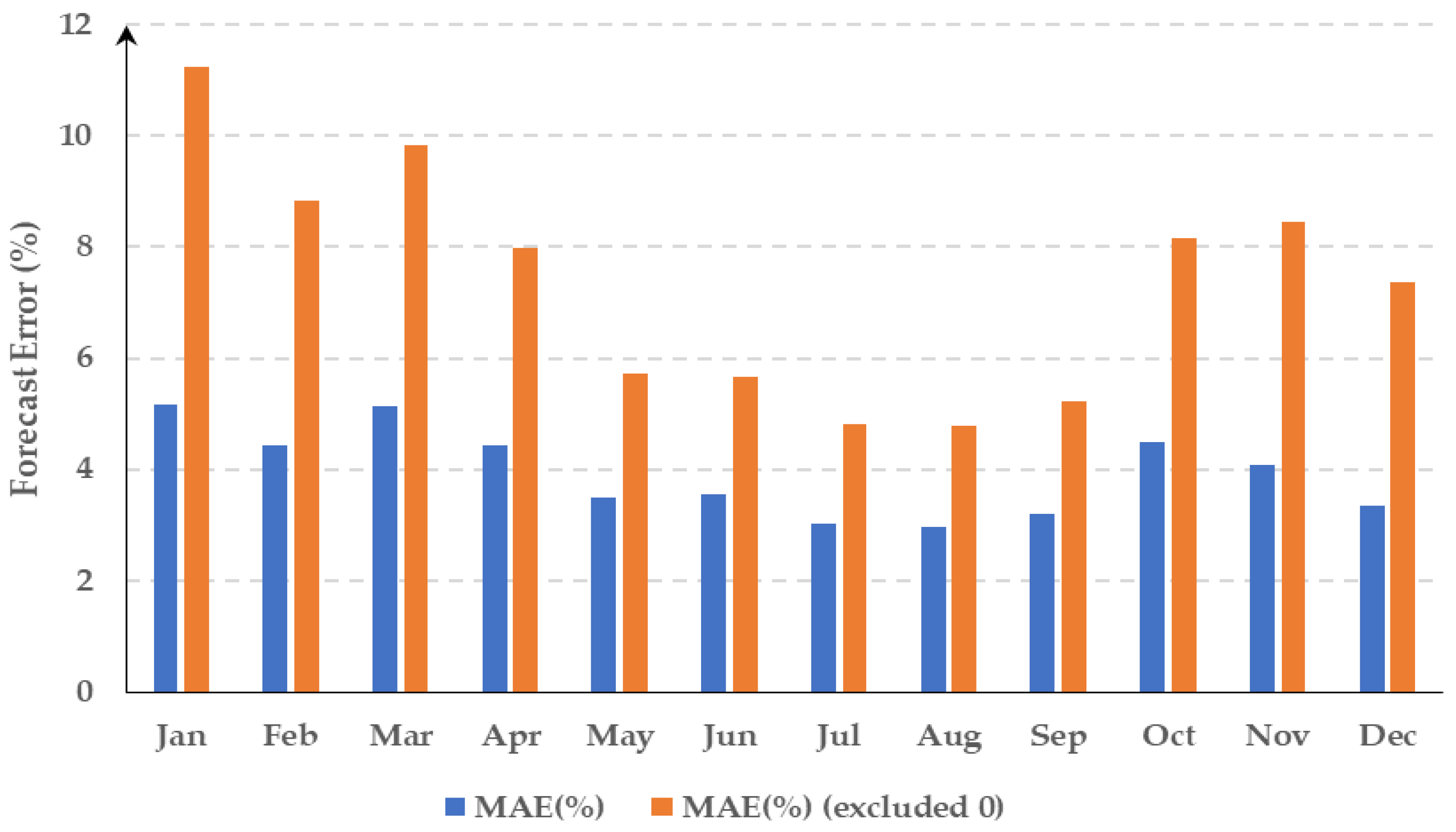
Normally, since the output is significantly more likely to be a 0 during periods when the sun does not rise, we considered the NMAE of the forecasting model except when both the forecast and measured values were 0. Figure 10 expresses the forecast error with and without 0 outputs. Additionally, the NMAE of the forecasting model for the year of 2016 is about 4%, and the accuracy for summer is better than that for winter.
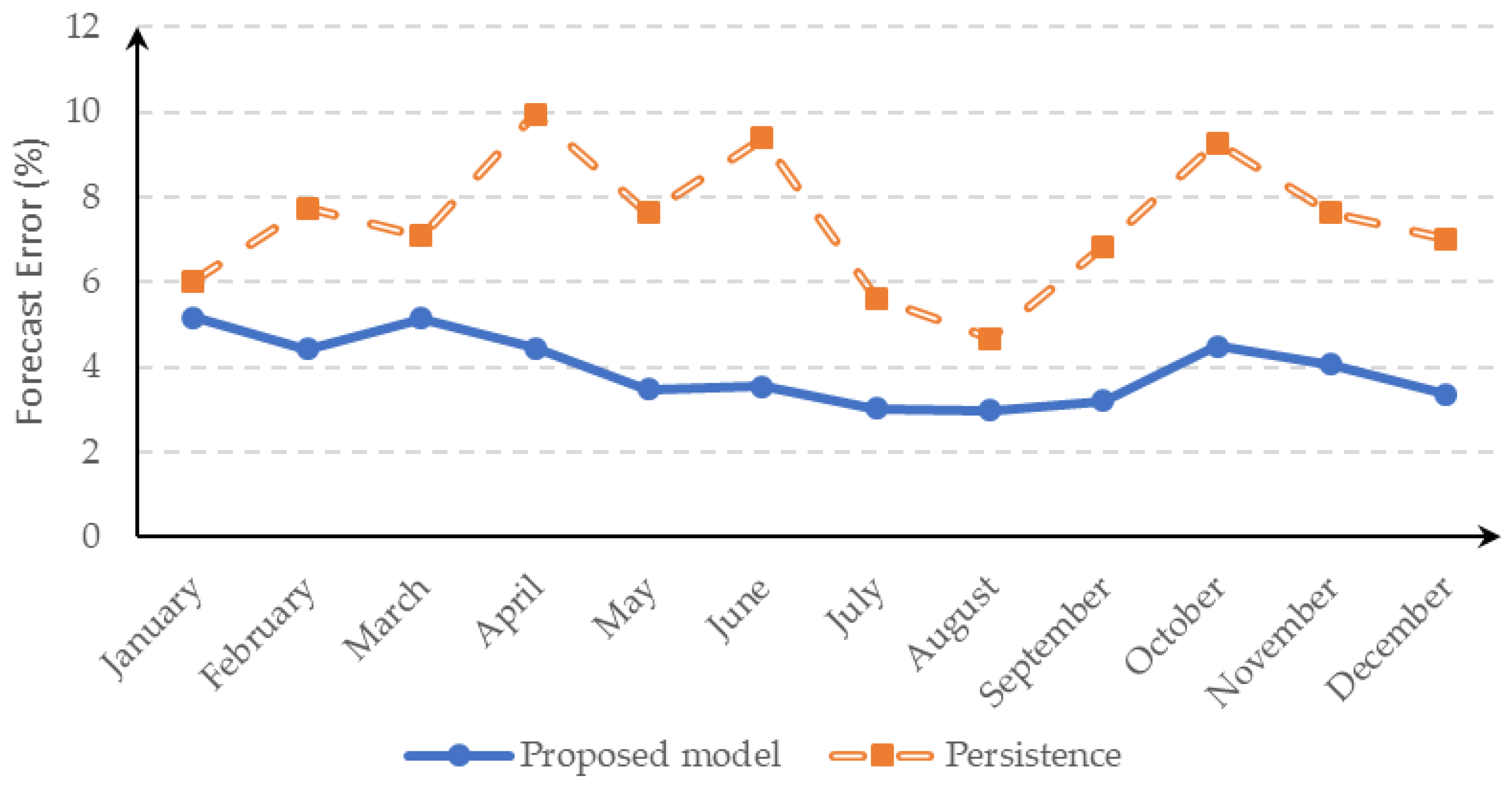
Several North American utilities have been forecasting solar power since the 2000s. Most operating entities use NMAE as a forecasting error assessment; as shown in Table 5, they had levels below 10% in 2013 [37]. In this paper, we identified an improvement in the proposed model compared to the persistence model, as shown in Figure 11 and Table 6.
4. Conclusions
As solar energy depends on climate phenomena, accurate forecasting technologies for stable interconnection of solar power generation are becoming increasingly important. In this paper, we proposed a probabilistic solar power output forecast method using a hybrid spatio-temporal forecasting model. We applied two estimating techniques to forecast the output of a solar power farm. Firstly, since numerical weather prediction models are difficult to apply in forecasting, kriging helps to perform spatial modeling for sites of interest using data from nearby points, as noted in Section 2.1. The results of the method give us relatively precise weather information. Secondly, we applied the Naïve Bayes Classifier method based on the probability. Unlike previous studies in which weather values were difficult to apply at the exact point and where discrete values were used, the proposed model allows for the consideration of meteorological values that are not applied to the classifier because of the continuous probability distribution. Finally, we applied the hybrid spatio-temporal forecasting model using empirical data to a solar farm located in South Korea and evaluated the performance of the model. As a result, it was confirmed that the NMAE of the forecasting model had a value of less than 10%. The proposed forecasting model based on a probabilistic approach shows improved results when compared to the deterministic persistence forecasting model.
In future, we will carry out probabilistic forecasting model improvements using a different probability distribution that will be used to better reflect the characteristics of the data. Also, we will represent a probabilistic range to ensure better results.
Author Contributions
J.H. conceived and designed the overall research; S.N. implemented the probabilistic forecasting model and conducted the experimental simulation; J.H. and S.N. wrote the paper; and J.H. guided the research direction and supervised the entire research process.
Acknowledgments
This research was supported by the MSIP (Ministry of Science, ICT and Future Planning), Korea, under the ITRC (Information Technology Research Center) support program (2015-0-00445) supervised by the IITP (Institute for Information.
Conflicts of Interest
The authors declare no conflict of interest.
References
- International Renewable Energy Agency. Renewable Capacity Highlights 2018. Available online: https://www.irena.org/-/media/Files/IRENA/Agency/Publication/2018/Mar/RE_capacity_highlights_2018.pdf (accessed on 25 September 2018).
- PJM. PJM’s Evolving Resource Mix and System Reliability. 2017. Available online: https://www.pjm.com/~/media/library/reports-notices/special-reports/20170330-appendix-to-pjms-evolving-resource-mix-and-system-reliability.ashx (accessed on 20 September 2018).
- Chow, C.W.; Urquhart, B.; Lave, M.; Dominguez, A.; Kleissl, J.; Shields, J.; Washom, B. Intra-hour forecasting with a total sky imager at the UC San Diego solar energy tested. Sol. Energy 2011, 85, 2881–2893. [Google Scholar] [CrossRef]
- Yang, H.; Kurtz, B.; Nguyen, D.; Urquhart, B.; Chow, C.W.; Ghonima, M.; Kleissl, J. Solar irradiance forecasting using a ground-based sky imager developed at UC San Diego. Sol. Energy 2014, 103, 502–524. [Google Scholar] [CrossRef]
- Perez, R.; Kivalov, S.; Schlemmer, J.; Hemker, K.; Hoff, T. Parameterization of site-specific short-term irradiance variability. Sol. Energy 2011, 85, 1343–1353. [Google Scholar] [CrossRef]
- Inman, R.H.; Hugo, T.C.P.; Carlos, F.M.C. Solar forecasting methods for renewable energy integration. Prog. Energy Combust. Sci. 2013, 535–576. [Google Scholar] [CrossRef]
- NYISO. Solar Impact on Grid Operations—An Initial Assessment. 2016. Available online: http://www.nyiso.com/public/webdocs/markets_operations/services/planning/Documents_and_Resources/Special_Studies/Special_Studies_Documents/Solar%20Integration%20Study%20Report%20Final%20063016.pdf (accessed on 20 September 2018).
- Pelland, S.; Galanis, G.; Kallos, G. Solar and photovoltaic forecasting through post-processing of the global environmental multiscale numerical weather prediction model. Prog. Photovolt. Res. Appl. 2013, 21, 284–296. [Google Scholar] [CrossRef]
- Marquez, R.; Coimbra, C.F.M. Forecasting of global and direct solar irradiance using stochastic learning methods, ground experiments and the NWS database. Sol. Energy 2011, 85, 746–756. [Google Scholar] [CrossRef]
- Yang, D.; Jirutitijaroen, P.; Walsh, W.M. Hourly solar irradiance time series forecasting using cloud cover index. Sol. Energy 2012, 86, 3531–3543. [Google Scholar] [CrossRef]
- NREL. National Solar Radiation Data Base. Available online: https://rredc.nrel.gov/solar/old_data/nsrdb/ (accessed on 25 September 2018).
- Mandal, P.; Madhira, S.T.S.; Haque, A.U.; Meng, J.; Pineda, R.L. Forecasting power output of solar photovoltaic system using wavelet transform and artificial intelligence techniques. Procedia Comput. Sci. 2012, 12, 332–337. [Google Scholar] [CrossRef]
- Pedro, H.T.C.; Coimbra, C.F.M. Assessment of forecasting techniques for solar power production with no exogenous inputs. Sol. Energy 2012, 86, 2017–2028. [Google Scholar] [CrossRef]
- Marquez, R.; Pedro, H.T.C.; Coimbra, C.F.M. Hybrid solar forecasting method uses satellite imaging and ground telemetry as inputs to ANNs. Sol. Energy 2013, 92, 176–188. [Google Scholar] [CrossRef]
- Le, D.D.; Berizzi, A.; Bovo, C.; Ciapessoni, E.; Cirio, D.; Pitto, A.; Gross, G. A Probabilistic Approach to Power System Security Assessment under Uncertainty. In Proceedings of the 2013 IREP Symposium-Bulk Power Dynamics and Control, Rethymno, Greece, 25–30 August 2013. [Google Scholar]
- Murata, A.; Ohtake, H.; Oozeki, T. Modeling of uncertainty of solar Irradiance forecasts on numerical weather predictions with the estimation of multiple confidence intervals. Renew. Energy 2018, 117, 193–201. [Google Scholar] [CrossRef]
- Ramakrishna, R.; Scaglione, A.; Vittal, V. A Stochastic Model for Short-Term Probabilistic Forecast of Solar Photo-Voltaic Power. In Proceedings of the Asilomar Conference on Signals, Systems and Computers 2016, Pacific Grove, CA, USA, 6–9 November 2016. [Google Scholar]
- Abuella, M.; Chowdhury, B. Hourly probabilistic forecasting of solar power. In Proceedings of the 2017 North American Power Symposium, Morgantown, WV, USA, 17–19 September 2017. [Google Scholar]
- Lauret, P.; David, M.; Hugo, T.C.P. Probabilistic Solar Forecasting using Quantile Regression Models. Energies 2017, 10, 1591. [Google Scholar] [CrossRef]
- Massidda, L.; Marrocu, M. Quantile Regression Post-Processing of Weather Forecast for Short-Term Solar Power Probabilistic Forecasting. Energies 2018, 11, 1763. [Google Scholar] [CrossRef]
- Mohammed, A.A.; Aung, Z. Ensemble Learning Approach for Probabilistic Forecasting of Solar Power Generation. Energies 2016, 9, 1017. [Google Scholar] [CrossRef]
- Zhang, Y.; Wang, J. GEFCom2014 Probabilistic Solar Power Forecasting based on k-Nearest Neighbor and Kernel Density Estimator. In Proceedings of the IEEE International Conference on Power & Energy Society General Meeting, Denver, CO, USA, 26–30 July 2015. [Google Scholar]
- Hong, T.; Pinson, P.; Zareipour, H.; Troccoli, A.; Rob, J.H. Probabilistic energy forecasting: Global Energy Forecasting Competition 2014 and beyond. Int. J. Forecast. 2016, 32, 896–913. [Google Scholar] [CrossRef] [Green Version]
- Sharma, N.; Sharma, P.; Irwin, D.; Shenoy, P. Predicting Solar Generation from Weather Forecasts Using Machine Learning. Smart Grid Communications. In Proceedings of the 2011 IEEE International Conference, Brussels, Belgium, 17–20 October 2011. [Google Scholar]
- Zafarani, R.; Eftekharnejad, S.; Patel, U. Assessing the Utility of Weather Data for Photovoltaic Power Prediction 2018. Available online: https://arxiv.org/pdf/1802.03913.pdf (accessed on 23 September 2018).
- Nomiyama, F.; Asai, J.; Murakami, T.; Murata, J. A study on global solar radiation forecasting using weather forecast data. Circuits and Systems. In Proceedings of the 2011 IEEE 54th International Midwest Symposium, Seoul, Korea, 7–10 August 2011. [Google Scholar]
- Stein, M.L. Interpolation of Spatial Data: Some Theory for Kriging; Springer: New York, NY, USA, 1999. [Google Scholar]
- Cressie, N. Spatial Prediction and Ordinary Kriging. Math. Geol. 1988, 20, 405–421. [Google Scholar] [CrossRef]
- Yamamoto, J.K. An Alternative Measure of the Reliability of Ordinary Kriging Estimates. Math. Geol. 2000, 32, 489–509. [Google Scholar] [CrossRef]
- Bracale, A.; Caramia, P.; Carpinelli, G.; Fazio, A.R.D.; Ferruzzi, G. A Bayesian Method for Short-Term Probabilistic Forecasting of Photovoltaic Generation in Smart Grid Operation and Control. Energies 2013, 6, 733–747. [Google Scholar] [CrossRef] [Green Version]
- Visscher, R.D.; Delouille, V.; Dupont, P.; Deledalle, C.A. Supervised classification of solar features using prior information. J. Space Weather Space Clim. 2015, 5, A34. [Google Scholar] [CrossRef] [Green Version]
- Quek, Y.T.; Woo, W.L.; Logenthiran, T. A naïve Bayes Classification Approach for Short-Term Forecast of Photovoltaic System. In Proceedings of the Sustainable Energy and Environmental Sciences, Singapore, 6–7 May 2017. [Google Scholar]
- Davig, T.; Hall, A.S. Recession Forecasting Using Bayesian Classification. Available online: https://www.kansascityfed.org/publications/research/rwp/articles/2016/recession-forecasting-bayesian-classification (accessed on 25 September 2018).
- Raschka, S. Naïve Bayes and Text Classification 1–Introduction and Theory. 2014. Available online: https://arxiv.org/abs/1410.5329 (accessed on 10 September 2018).
- Kim, S.B.; Han, K.S.; Rim, H.C.; Myaeng, S.H. Some Effective Techniques for Naïve Bayes Text Classification. IEEE Trans. Knowl. Data Eng. 2006, 18, 1457–1466. [Google Scholar]
- Gayathri, A.; Revathi, M.; Velmurugan, J. A survey on Weather forecasting by Data Mining. IJARCCE 2016, 5, 298–300. [Google Scholar]
- Widiss, R.; Porter, K. A Review of Variable Generation Forecasting in the West. Available online: https://www.nrel.gov/docs/fy14osti/61035.pdf (accessed on 20 September 2018).
- Dolara, A.; Grimaccia, F.; Leva, S.; Mussetta, M. Comparison of Training Approaches for Photovoltaic Forecasts by Means of Machine Learning. Appl. Sci. 2018, 8, 228. [Google Scholar] [CrossRef]
Figure 1.
Algorithm for the hybrid spatio-temporal forecasting model.

Figure 2.
Visualization of the kriging technique.

Figure 3.
A Naïve Bayes Classifier Network.

Figure 4.
Location data of both 30 METs and the solar farm.

Figure 5.
Locations and weights of METs.

Figure 6.
Weather data estimated at solar farm “A” and measured at three highly weighted neighboring points for August 2016. (a) Irradiance; (b) Humidity; (c) Temperature.
Figure 6.
Weather data estimated at solar farm “A” and measured at three highly weighted neighboring points for August 2016. (a) Irradiance; (b) Humidity; (c) Temperature.


Figure 7.
Prior probability used in the simulation.

Figure 8.
Probability distribution of the irradiance given that the solar output is 4.9 MW.

Figure 9.
Comparison of the actual and forecast solar power in August 2016.

Figure 10.
Forecast error for solar power output in 2016.

Figure 11.
Monthly NMAE of each forecasting method for solar power output in 2016.


Table 1.
Location data of both 30 METs and the solar farm.
| Name | Longitude | Latitude |
|---|---|---|
| MET1 | 37.57 | 126.96 |
| MET2 | 37.47 | 126.92 |
| MET3 | 37.27 | 126.98 |
| MET4 | 37.33 | 127.94 |
| MET5 | 37.90 | 127.73 |
| MET6 | 37.67 | 128.71 |
| MET7 | 37.80 | 128.85 |
| MET8 | 37.75 | 128.89 |
| MET9 | 36.77 | 126.49 |
| MET10 | 36.63 | 127.44 |
| MET11 | 36.37 | 127.37 |
| MET12 | 34.81 | 126.38 |
| MET13 | 35.28 | 126.47 |
| MET14 | 35.84 | 127.11 |
| MET15 | 35.37 | 127.12 |
| MET16 | 35.17 | 126.89 |
| MET17 | 34.94 | 127.69 |
| MET18 | 34.62 | 126.76 |
| MET19 | 34.76 | 127.21 |
| MET20 | 35.42 | 126.69 |
| MET21 | 35.10 | 129.03 |
| MET22 | 36.22 | 127.99 |
| MET23 | 36.57 | 128.70 |
| MET24 | 36.43 | 129.04 |
| MET25 | 35.51 | 127.74 |
| MET26 | 35.81 | 129.20 |
| MET27 | 35.32 | 128.28 |
| MET28 | 35.16 | 128.04 |
| MET29 | 35.22 | 128.67 |
| MET30 | 35.22 | 128.89 |
| Solar Farm | 35.22 | 126.31 |
Table 2.
Weights of 30 METs for solar farm “A”.
| Neighbor Point | Weight | Neighbor Point | Weight | Neighbor Point | Weight |
|---|---|---|---|---|---|
| MET1 | 0.016438 | MET11 | 0.018432 | MET21 | 0.017088 |
| MET2 | 0.018829 | MET12 | 0.123704 | MET22 | 0.024010 |
| MET3 | 0.017793 | MET13 | 0.379523 | MET23 | 0.020570 |
| MET4 | 0.023736 | MET14 | 0.021432 | MET24 | 0.020350 |
| MET5 | 0.023736 | MET15 | 0.020195 | MET25 | 0.021448 |
| MET6 | 0.015201 | MET16 | -0.01156 | MET26 | 0.023946 |
| MET7 | 0.012228 | MET17 | 0.020206 | MET27 | 0.017606 |
| MET8 | 0.012259 | MET18 | 0.008242 | MET28 | 0.015003 |
| MET9 | 0.024126 | MET19 | 0.022546 | MET29 | 0.014557 |
| MET10 | 0.019265 | MET20 | 0.026276 | MET30 | 0.012812 |
Table 3.
Cross validation error for irradiance of five METs.
| Neighbor Point | Error (%) |
|---|---|
| MET1 | 15.2875 |
| MET4 | 19.6477 |
| MET9 | 19.2359 |
| MET13 | 15.0040 |
| MET22 | 15.1128 |
Table 4.
The normalized mean absolute error (NMAE) for each month of forecasting in 2016.
| Month | NMAE (%) | Month | NMAE (%) |
|---|---|---|---|
| January | 5.159702 | July | 3.017107 |
| February | 4.423764 | August | 2.969330 |
| March | 5.136241 | September | 3.212500 |
| April | 4.444066 | October | 4.488025 |
| May | 3.479961 | November | 4.068056 |
| June | 3.540152 | December | 3.355083 |
Table 5.
Assessments of forecasting accuracy.
| Operation Entity | 2013 Value |
|---|---|
| CASIO | MAE < 8% |
| Idaho Power | MAE < 6.5% |
| Xcel Energy | MAE < 9.8% |
Table 6.
NMAE for each month of forecasting in 2016.
| Month | Proposed Model | Persistence |
|---|---|---|
| January | 5.159702 | 6.0136 |
| February | 4.423764 | 7.7273 |
| March | 5.136241 | 7.0781 |
| April | 4.444066 | 9.9371 |
| May | 3.479961 | 7.6248 |
| June | 3.540152 | 9.3845 |
| July | 3.017107 | 5.6085 |
| August | 2.969330 | 4.6752 |
| September | 3.212500 | 6.8424 |
| October | 4.488025 | 9.2645 |
| November | 4.068056 | 7.6265 |
| December | 3.355083 | 7.0162 |
© 2018 by the authors. Licensee MDPI, Basel, Switzerland. This article is an open access article distributed under the terms and conditions of the Creative Commons Attribution (CC BY) license (http://creativecommons.org/licenses/by/4.0/).
Share and Cite
MDPI and ACS Style
Nam, S.; Hur, J. Probabilistic Forecasting Model of Solar Power Outputs Based on the Naïve Bayes Classifier and Kriging Models. Energies 2018, 11, 2982. https://0-doi-org.brum.beds.ac.uk/10.3390/en11112982
AMA Style
Nam S, Hur J. Probabilistic Forecasting Model of Solar Power Outputs Based on the Naïve Bayes Classifier and Kriging Models. Energies. 2018; 11(11):2982. https://0-doi-org.brum.beds.ac.uk/10.3390/en11112982
Chicago/Turabian StyleNam, Seungbeom, and Jin Hur. 2018. "Probabilistic Forecasting Model of Solar Power Outputs Based on the Naïve Bayes Classifier and Kriging Models" Energies 11, no. 11: 2982. https://0-doi-org.brum.beds.ac.uk/10.3390/en11112982
Note that from the first issue of 2016, this journal uses article numbers instead of page numbers. See further details here.