Decomposition and Forecasting of CO₂ Emissions in China’s Power Sector Based on STIRPAT Model with Selected PLS Model and a Novel Hybrid PLS-Grey-Markov Model

Abstract

China faces significant challenges related to global warming caused by CO₂ emissions, and the power industry is a large CO₂ emitter. The decomposition and accurate forecasting of CO₂ emissions in China’s power sector are thus crucial for low-carbon outcomes. This paper selects seven socio-economic and technological drivers related to the power sector, and decomposes CO₂ emissions based on two models: the extended stochastic impacts by regression on population, affluence and technology (STIRPAT) model and the partial least square (PLS) model. Distinguished from previous research, our study first compares the effects of eliminating the multicollinearity of the PLS model with stepwise regression and ridge regression, finding that PLS is superior. Further, the decomposition results show the factors’ absolute elasticity coefficients are population (2.58) > line loss rate (1.112) > GDP per capita (0.669) > generation structure (0.522) > the urbanization level (0.512) > electricity intensity (0.310) > industrial structure (0.060). Meanwhile, a novel hybrid PLS-Grey-Markov model is proposed, and is verified to have better precision for the CO₂ emissions of the power sector compared to the selected models, such as ridge regression-Grey-Markov, PLS-Grey-Markov, PLS-Grey and PLS-BP (Back propagation neutral network model). The forecast results suggest that CO₂ emissions of the power sector will increase to 5102.9 Mt by 2025. Consequently, policy recommendations are proposed to achieve low-carbon development in aspects of population, technology, and economy.

1. Introduction

The impacts of climate change have become increasingly severe, arousing extensive attention worldwide [1,2,3]. Global warming is mostly attributed to greenhouse gas (GHG) emissions, especially CO₂ originating from enhanced industrialization [4,5]. Substantial CO₂ emissions can bring about adverse effects on the natural environment. Moreover, the use of fossil fuel is the main origin of CO₂ emissions, which poses significant challenges to environmental protection in the context of securing worldwide energy supplies [6].

The power industry converts primary energy sources, such as coal, into electrical energy, which plays a natural monopoly role within the energy sector [7]. The electricity industry is not only the crucial energy sector in the process of economic growth, but also an industry fundamental to people’s livelihoods [8]. The electricity industry is a substantial energy-related CO₂ emitter, and its global emissions proportion has risen from 36% in 1990, to 42% in 2014, and is predicted to rise to 45% in 2030 [9].

China has become the largest CO₂ emitter globally. It joined “The Paris Agreement” to jointly develop measures for coping with greenhouse effects after 2020 [4]. Owing to China’s resource endowment and energy structure, its CO₂ emissions from fuel consumption increased to 9134.9 Mt in 2014, a 333% increase compared with 1990 [9]. China’s power sector ranked first in terms of its share of national CO₂ emissions, accounting for 48.79% of the total [10]. A reduction of CO₂ emissions by China’s power industry is, hence, a key factor for achieving low-carbon development, which, in turn, is of great importance for decision-makers within China’s government who aim to implement appropriate environmental policy [11].

Literature related to CO₂ emissions in China can be generally classified as having either all-industries or single-industry approaches. Many scholars have researched energy consumption in China from the all-industries perspective, and previous studies paid attention to analysis of the driving factors of CO₂ emissions. Yang et al. [12] researched net CO₂ emissions with the help of the logarithmic mean Divisia index (LMDI) model in the Wuhan Metropolitan district. Zha et al. [13] applied the LMDI model to probe into the factors which may impact changes in CO₂ emissions from urban and rural residential energy consumption. Li et al. [14] utilized the stochastic impacts by regression on population, affluence and technology (STIRPAT) model to access drivers on provincial CO₂ emissions per capita, demonstrating that urbanization level and GDP per capita had stronger effects on CO₂ emissions. Feng et al. [15] adopted a system dynamics method to examine the impacts of drivers of energy consumption and the trend of CO₂ emissions in Beijing. Wang and Liu [16] utilized a spatiotemporal method to explore the driving factors of China’s city-level CO₂ emissions and found an inverted U-shaped relation between CO₂ emissions per capita and economic growth. Mi et al. applied a structural decomposition analysis to study the determinants of China’s carbon emissions [17]. There are also some studies aimed at CO₂ emissions prediction. Bao and Hui [18] used a GM (1, 1) model (grey model of 1st order and 1 variable) to research CO₂ emissions in Shijiazhuang city, and the result revealed that the GM (1, 1) method had better fitting precision. Ding et al. [19] predicted the CO₂ emissions from fuel combustion by means of the original multi-variable grey approach. Zhao et al. [20] applied the SSA-LSSVM (Least squares support vector machine for singular spectrum analysis) model to predict energy-related CO₂ emissions, indicating structural factors prominently affect CO₂ emission forecast results. Dai et al. [21] used the GM (1, 1) and LSSVM model to predict CO₂ emissions in China.

Literature concerning CO₂ emissions at the all-industries level provided macro conclusions which were not applicable to individual industries throughout China. Thus, scholars also focused more concretely on several industries. Zhang et al. [22] studied energy-related CO₂ emissions from all major industrial sectors of China based on decomposition analysis. The results concluded that China had made a remarkable contribution to reducing global CO₂ emissions. Wu and Shi [23] examined the use of energy for tourism and concluded tourism was a low-carbon industry and also a pillar industry in terms of reduction of CO₂ emissions. Zhang et al. [24] illustrated that the total-factor CO₂ emissions of China’s transportation sector diminished by 32.8% during the study period. Cui et al. [4] estimated carbon emissions in Hebei Province based on the STIRPAT model, showing that production efficiency was the primary driving factor causing agricultural carbon emissions. Zhao et al. [25] adopted the STIRPAT model to study the major drivers affecting the energy-related carbon emissions of the transportation sector in Guangdong. Yao et al. [26] used the meta-frontier non-radial Malmquist CO₂ emission performance index to calculate the trends of China’s provincial industrial sector and their driving forces.

In terms of China’s power generation industry, Zhang [27] identified the determinants of CO₂ emissions change of the power sector in Beijing-Tianjin-Hebei region, and showed that the production sector’s electricity intensity remains a critical factor for achieving CO₂ emission reductions. Sun et al. [28] used a scenario analysis approach to estimate the CO₂ emissions in China’s power industry for diverse scenarios, and derived policy implications based on the extended STIRPAT model. Wen et al. [29] explored drivers of CO₂ emissions in China’s power sector based on ridge regression and proposed related policy measures. Zhao et al. [30] applied ridge regression analysis and a neural network optimized by a Gauss prediction model to predict the CO₂ emissions of the power sector. Lindner et al. [31] estimated direct CO₂ emissions deriving from electrical exports and imports among China’s provinces.

Reviewing previous research, most literature has mostly concentrated on the impacts of socio-economic progress on CO₂ emissions. However, the drivers affecting CO₂ emissions are various, and not only involve macro development, but also electricity productive activities. Moreover, previous studies have focused solely on the driving factor decomposition or prediction of CO₂ emissions in the power sector, and have not verified the quality of the driving factor decomposition model. Therefore, it is vital to control CO₂ emissions caused by the electric power industry and to investigate factors affecting CO₂ emissions compared with the common model. In addition, high-precision measurement of the CO₂ emissions of China’s power industry is significant for accurate weather monitoring and control of air pollution. Therefore, uniformly combining factor decomposition with predictive analysis in the power sector is beneficial to the reduction of CO₂ emissions and the achievement of low-carbon development in China.

In summary, to contribute to filling the gaps in the existing literature, this study is conducted as follows. First, we use the STIRPAT model to probe into determinants of CO₂ emissions from China’s power sector. We also use the PLS model to eliminate multicollinearity, compared with stepwise regression and ridge regression. Second, considering the relatively few data and good forecast results, a Grey-Markov model is established to accurately forecast influencing factors, compared with a GM (1, 1) model and a BP neural network. Third, we obtain high-precision estimates of the CO₂ emissions of China’s power industry based on a PLS-Grey-Markov model. Finally, conclusions and policy recommendations to boost low-carbon development in China are presented based on model results. These are essential for controlling CO₂ emissions and deserve further study for other industries.

Hence, this paper distinguishes from the existing literature in the following aspects: (1) We select seven socio-economic and technology drivers related to the whole electricity sector to explore the mechanism driving CO₂ emissions by means of the extended STIRPAT model and PLS model. In particular, in contrast to previous studies that have solely regarded socio-economic factors, some specific technology drivers involved in the power production, such as line loss rate and electricity intensity, are included to investigate their effects on CO₂ emissions. (2) This is the first comparison of the effects of eliminating the multicollinearity of the PLS model, stepwise regression and ridge regression, in order to judge the superior quality of the PLS model. (3) The study is also the first to establish a novel hybrid PLS-Grey-Markov optimized approach, which is based on both the PLS and Grey-Markov models. The result appears to be highly beneficial and shows significant improvement for forecasting CO₂ emissions of China’s power sector.

2. Methodology

This section mainly introduces the PLS, GM (1, 1), and Grey-Markov models and error measures used in this paper.

2.1. PLS Model

The PLS method is identified by Wold et al. as a particularly useful multivariate statistical analysis method [32]. It surmounts the issue of multicollinearity because of the comprehensive means of extracting components and information and its screening methodology [33].

The main operation of the PLS model is to extract the integrated variables ${\mathrm{t}}_1$ and ${\mathrm{u}}_1$ from the data table of explanatory variables $\mathrm{X}$ and the explained variable $\mathrm{Y}$, where ${\mathrm{t}}_1$ and ${\mathrm{u}}_1$ are the linear incorporation of ${\mathrm{x}}_1,{\mathrm{x}}_2,\dots ,{\mathrm{x}}_{\mathrm{p}}$ and ${\mathrm{y}}_1,{\mathrm{y}}_2,\dots ,{\mathrm{y}}_{\mathrm{p}}$, respectively. Specifically, ${\mathrm{t}}_1$ and ${\mathrm{u}}_1$ should satisfy the following conditions:

(1) ${\mathrm{t}}_1$ and ${\mathrm{u}}_1$ should contain as much of their original variation information as possible for representing data tables $\mathrm{X}$ and $\mathrm{Y}$ more adequately;

(2) ${ \mathrm{t}}_1$ and ${\mathrm{u}}_1$ should attain the maximum degree of correlation, which offers ${\mathrm{t}}_1$ the greatest explanatory power to ${\mathrm{u}}_1$.

If the result of regression precision is satisfactory, the procedure will be terminated; if unsatisfactory, the second component ${\mathrm{t}}_1$ should be extracted from the remaining information of $\mathrm{X}$ and the second regression analysis is conducted. The regression is repeatedly executed until the satisfactory precision is obtained and the latent variables ${\mathrm{t}}_1,{\mathrm{t}}_2,\dots ,{\mathrm{t}}_{\mathrm{m}}$ are obtained.

2.2. GM (1, 1) Model

The grey system was firstly proposed by Deng [34]. The grey forecasting model is applied in cases with fewer data, and is used for prediction in a complex environment where policy-makers have limited historical data. The kernel of GM (1, 1) is shown as follows:

Step 1: The non-negative raw time-series ${\mathrm{X}}^{(0)}$ is defined as:

$${\mathrm{X}}^{(0)}=\left\{{\mathrm{X}}^{(0)}(1),{\mathrm{X}}^{(0)}(2),\dots ,{\mathrm{X}}^{(0)}(\mathrm{n})\right\},{\mathrm{X}}^{(0)}(\mathrm{k})>0,\mathrm{k}=1,2,\dots ,\mathrm{n}.$$

(1)

Step 2: A new series ${\mathrm{X}}^{(1)}$ can be obtained by taking accumulated generating operation (AGO) on ${\mathrm{X}}^{(0)}$:

$${\mathrm{X}}^{(1)}=\left\{{\mathrm{X}}^{(1)}(1),{\mathrm{X}}^{(1)}(2),\dots ,{\mathrm{X}}^{(1)}(\mathrm{n})\right\}$$

(2)

where ${\mathrm{X}}^{(1)}(\mathrm{k})={\sum }_{\mathrm{i}=1}^{\mathrm{k}}{\mathrm{X}}^{(0)}(\mathrm{i}),\mathrm{k}=1,2,\dots ,\mathrm{n}.$

Step 3: The basic form of the GM (1, 1) model is obtained by:

$$\frac{{\mathrm{dX}}^{(1)}}{\mathrm{dt}}+{\mathrm{aX}}^{(1)}=\mathrm{b}$$

(3)

where $\mathrm{a}$ represents the developing coefficient and $\mathrm{b}$ denotes the grey input. Parameter $\hat{\mathrm{a}}$ is represented by:

$$\hat{\mathrm{a}}={({\mathrm{B}}^{\mathrm{T}}\mathrm{B})}^{-1}{\mathrm{B}}^{\mathrm{T}}\mathrm{Y}$$

(4)

where $\mathrm{B}=[\begin{array}{cccc}-\frac{1}{2}({\mathrm{X}}^{(1)}(1)+{\mathrm{X}}^{(1)}(2))& 1& \dots & 1\\ -\frac{1}{2}({\mathrm{X}}^{(1)}(2)+{\mathrm{X}}^{(1)}(3))& 1& \dots & 1\\ ⋮& ⋮& ⋮& ⋮\\ -\frac{1}{2}({\mathrm{X}}^{(1)}(\mathrm{n}-1)+{\mathrm{X}}^{(1)}(\mathrm{n}))& 1& \dots & 1\end{array}]$, and ${\mathrm{Y}}_{\mathrm{n}}={[{\mathrm{X}}_1^{(0)}(2),{\mathrm{X}}_1^{(0)}(3),\dots ,{\mathrm{X}}_1^{(0)}(\mathrm{n})]}^{\mathrm{T}}$

Step 4: Based on the estimated coefficients of $\mathrm{a}$ and $\mathrm{b}$, the response equation and the prediction value can be achieved by:

$$\begin{gathered} {\hat{\mathrm{X}}}^{(1)}(\mathrm{k}+1)=({\mathrm{X}}^{(1)}(0)-\frac{\mathrm{b}}{\mathrm{a}}){\mathrm{e}}^{-\mathrm{ak}}+\frac{\mathrm{b}}{\mathrm{a}} \\ {\hat{\mathrm{X}}}^{(0)}(\mathrm{k}+1)={\hat{\mathrm{X}}}^{(1)}(\mathrm{k}+1)-{\hat{\mathrm{X}}}^{(1)}(\mathrm{k}),\mathrm{k}=1,2,\dots ,\mathrm{n}. \end{gathered}$$

(5)

2.3. Grey-Markov Model

The forecasting accuracy of the GM (1, 1) prediction model is weak in data series with significant fluctuations. The Markov-chain prediction model can be applied to forecast a system with randomly dynamic data series. Hence, the Markov-chain model enhances the GM (1, 1) model if fluctuation in the dataset is relatively large [35]. The Grey-Markov model [36] is an particular form of stochastic process, which has been widely utilized to build stochastic models in diverse disciplines. Further, Markov chain is a prediction approach to forecast data from previous events.

The simulation sequence can be obtained by means of Equation (5) as follows:

$${\hat{\mathrm{X}}}^{(0)}=\left\{{\hat{\mathrm{X}}}^{(0)}(1),{\hat{\mathrm{X}}}^{(0)}(2),\dots {\hat{\mathrm{X}}}^{(0)}(\mathrm{n})\right\}$$

(6)

The procedure of the Grey-Markov model can be summarized as follows:

Step 1: Compute the relative error (RE) on the basis of the following equation:

$$\mathsf{\epsilon }(\mathrm{k})=\frac{{\mathrm{X}}^{(0)}(\mathrm{k})-{\hat{\mathrm{X}}}^{(0)}(\mathrm{k})}{{\mathrm{X}}^{(0)}(\mathrm{k})}\ast 100\%$$

(7)

Based on the maximum and minimum of the RE, the residual series are appropriately separated into several intervals that can be considered as the state vector $\mathrm{E}=\left[{\mathrm{E}}_{1,}{\mathrm{E}}_2,\dots ,{\mathrm{E}}_{\mathrm{m}}\right]$ of the Markov chain:

$$\mathrm{E}=\left[{\mathrm{E}}_{\mathrm{i}-,},{\mathrm{E}}_{\mathrm{i}+}\right],{\mathrm{E}}_{\mathrm{i}-,}={\hat{\mathrm{X}}}^{(0)}(\mathrm{k})+{\mathrm{A}}_{\mathrm{i}},{\mathrm{E}}_{\mathrm{i}+}{\hat{\mathrm{X}}}^{(0)}(\mathrm{k})+{\mathrm{B}}_{\mathrm{i}}$$

(8)

Step 2: Calculate the state transition probability ${\mathrm{P}}_{\mathrm{ij}}^{(\mathrm{k})}$, which represents the probability from ${\mathrm{E}}_{\mathrm{i}}$ to ${\mathrm{E}}_{\mathrm{j}}$ after $\mathrm{k}$ steps. The transition time is ${\mathrm{t}}_1,{\mathrm{t}}_2,\dots ,{\mathrm{t}}_{\mathrm{n}}$, so the k-step transition probability can be achieved by:

$${\mathrm{P}}_{\mathrm{ij}}^{(\mathrm{k})}=\frac{{\mathrm{n}}_{\mathrm{ij}}^{(\mathrm{k})}}{{\mathrm{N}}_{\mathrm{i}}}$$

$$\sum _{\mathrm{j}=1}^{\mathrm{m}}{\mathrm{P}}_{\mathrm{ij}}^{(\mathrm{k})}=1;\mathrm{i},\mathrm{j}=1,2,\dots ,\mathrm{m}.$$

(9)

where ${\mathrm{N}}_{\mathrm{i}}$ indicates the data number at which the stochastic process state is ${\mathrm{E}}_{\mathrm{i}}$, and the ${\mathrm{n}}_{\mathrm{ij}}^{(\mathrm{k})}$ denotes the transition number from ${\mathrm{E}}_{\mathrm{i}}$ to ${\mathrm{E}}_{\mathrm{j}}$ in k steps. The matrix of k-step transition probability can be expressed as follows:

$${\mathrm{P}}^{(\mathrm{k})}=\left[\begin{array}{cc}\begin{array}{cc}{\mathrm{P}}_{11}^{(\mathrm{k})}& {\mathrm{P}}_{12}^{(\mathrm{k})}\\ {\mathrm{P}}_{21}^{(\mathrm{k})}& {\mathrm{P}}_{22}^{(\mathrm{k})}\end{array}& \begin{array}{cc}\begin{array}{c}\cdots \\ \cdots \end{array}& \begin{array}{c}{\mathrm{P}}_{1\mathrm{m}}^{(\mathrm{k})}\\ {\mathrm{P}}_{2\mathrm{m}}^{(\mathrm{k})}\end{array}\end{array}\\ \begin{array}{cc}⋮& ⋮\\ {\mathrm{P}}_{\mathrm{m}1}^{(\mathrm{k})}& {\mathrm{P}}_{\mathrm{m}2}^{(\mathrm{k})}\end{array}& \begin{array}{cc}⋮& ⋮\\ \cdots & {\mathrm{P}}_{\mathrm{mm}}^{(\mathrm{k})}\end{array}\end{array}\right]$$

(10)

The future process of the system is predicted by deriving the state transition probability matrix ${\mathrm{P}}^{(\mathrm{k})}$. In general, it is essential and useful to survey the one-step transition matrix ${\mathrm{P}}^{(1)}$. Supposing that the target predicted is in state ${\mathrm{E}}_{\mathrm{q}}(1\le \mathrm{q}\le \mathrm{m})$, the row $\mathrm{q}$ in matrix ${\mathrm{P}}^{(1)}$ should be considered. If max ${\mathrm{p}}_{\mathrm{q}\mathrm{j}}^{(1)}={\mathrm{p}}_{\mathrm{q}\mathrm{l}}^{(1)}(\mathrm{j}=1,2,\dots ,\mathrm{m},(1\le \mathrm{q}\le \mathrm{m}))$, then the transition from state ${\mathrm{E}}_{\mathrm{q}}$ to state ${\mathrm{E}}_{\mathrm{l}}$ will possibly occur to a large degree in the next moment.

Step 3: Calculate the modified forecasting values. After determining the future state transition of a system, the related residual error zone $\mathrm{E}=\left[{\mathrm{E}}_{\mathrm{i}-,},{\mathrm{E}}_{\mathrm{i}+}\right]$ is attained, and the median of $\mathrm{E}=\left[{\mathrm{E}}_{\mathrm{i}-,},{\mathrm{E}}_{\mathrm{i}+}\right]$ is chosen as the relative error. Thus, the modified prediction value of primal data sequence is gained with the help of the above explanation as:

$${\mathrm{X}}^{\stackrel{`}{(}0)}(\mathrm{k}+1)=\frac{1}{2}({\mathrm{E}}_{\mathrm{i}-,}+{\mathrm{E}}_{\mathrm{i}+})={\hat{\mathrm{X}}}^{(0)}(\mathrm{k})+\frac{1}{2}({\mathrm{A}}_{\mathrm{i}}+{\mathrm{B}}_{\mathrm{i}})$$

(11)

2.4. Error Measures

To test and verify the rationality of data processing, we select mean absolute error (MAE), mean absolute percentage error (MAPE) and root-mean-square error (RMSE) to demonstrate the performance of the PLS-Grey-Markov model. The specific formulae are:

$$\mathrm{MAE}=\frac{1}{\mathrm{n}}\sum _{\mathrm{i}=1}^{\mathrm{n}}\left|\widehat{{\mathrm{y}}_{\mathrm{i}}}-{\mathrm{y}}_{\mathrm{i}}\right|$$

(12)

$$\mathrm{MAPE}=\frac{1}{\mathrm{n}}\sum _{\mathrm{i}=1}^{\mathrm{n}}(\left|\frac{\widehat{{\mathrm{y}}_{\mathrm{i}}}-{\mathrm{y}}_{\mathrm{i}}}{{\mathrm{y}}_{\mathrm{i}}}\right|\ast 100)$$

(13)

$$\mathrm{MAE}=\frac{1}{\mathrm{n}}\sqrt{\frac{1}{\mathrm{n}}\sum _{\mathrm{i}=1}^{\mathrm{n}}{(\widehat{{\mathrm{y}}_{\mathrm{i}}}-{\mathrm{y}}_{\mathrm{i}})}^2}$$

(14)

where $\widehat{{\mathrm{y}}_{\mathrm{i}}}$, ${\mathrm{y}}_{\mathrm{i}}$ are forecast and value, respectively.

3. Data Illustration and Collection

This section details the model for selecting variables, the calculation of carbon dioxide emissions in the power industry, and the collection of data.

3.1. STIRPAT Model

To study drivers of the environment, Enrlich and Holdren first put forward the IPAT method [37]:

$$\mathrm{I}=\mathrm{PAT}$$

(15)

where I denotes CO₂ emissions, P denotes total population, A represents affluence, and T refers to technology. In the hypothesized IPAT model, I is affected equally proportionally by the drivers, violating the reality condition [38]. Hence, Dietz and Rosa proposed a modified model named the STIRPAT model [39]:

$$\mathrm{I}={\mathrm{aP}}^{\mathrm{b}}{\mathrm{A}}^{\mathrm{c}}{\mathrm{T}}^{\mathrm{d}}\mathrm{e}$$

(16)

where I, P, A, and T are the identical independent variables in Equation (15), a denotes the whole model coefficient, b, c and d denote exponents of each explanatory variable respectively, and e refers to the error item [5]. The natural logarithm form of STIRPAT model is:

$$\ln (\mathrm{I})=\ln (\mathrm{a})+\mathrm{bln}(\mathrm{P})+\mathrm{cln}(\mathrm{A})+\mathrm{dln}(\mathrm{T})+\ln (\mathrm{e})$$

(17)

When other variables are unchanging, 1% variation of P, A, and T, respectively, will cause b%, c%, and d% change of I. In addition, the STIRPAT model can be extended by adding extra variables for studying more probable factors pertaining to CO₂ emissions [40]. For the purpose of investigating the effects of the drivers of the CO₂ emissions of the power industry, considering the specific development situation and learning from relevant research experience, a few more factors have been included [41,42].

CO₂ emissions can be seen as a type of environmental influence due to their impact on climate change. To explore the drivers of CO₂ emissions from the power sector, taking the real-world situation and relevant literature into consideration, other factors have been added in this paper. Drivers influencing CO₂ emissions are classified under four headings. The first is population, represented by total population or urbanization level in earlier literature, which are found to be the contributory drivers of CO₂ emissions [27,28,29,30,41,42,43,44]. The second is affluence, usually reflected by gross domestic product (GDP) per capita. The third is structure: the percentage of secondary industry output to total GDP is used to indicate the industrial structure, and the generation structure is the share of thermal power generation within total electricity generation [29]. Both reflect the proportion of high-pollution industry or power generation. The fourth is technology, represented by electricity intensity and line loss rate. Electricity intensity can represent power consuming efficiency, and the line loss rate is the percentage of the electricity loss over the total power generation in the power grid. Hence, the STIRPAT model can be extended as follows:

$$\ln ({\mathrm{CO}}_2)=\ln (\mathrm{a})+{\mathsf{\beta }}_1\ln (\mathrm{P})+{\mathsf{\beta }}_2\ln (\mathrm{PGDP})+{\mathsf{\beta }}_3\ln (\mathrm{GS})+{\mathsf{\beta }}_4\ln (\mathrm{IS})+{\mathsf{\beta }}_5\ln (\mathrm{EI})+{\mathsf{\beta }}_6\ln (\mathrm{LLR})+{\mathsf{\beta }}_7\ln (\mathrm{URB})+\ln (\mathrm{e})$$

(18)

Descriptions of each variable are listed in

Table 1. Description of variables in this paper.

Factors	Symbol	Definition	Unit
CO2 emissions	CO2	CO2 emissions from power industry	Million tons
Population	P	Total population	104 people
Economic activity	PGDP	GDP per capita	Yuan
Generation structure	GS	The proportion of thermal power generation within total electricity generation	%
Industrial structure	IS	The share of secondary industry output in total GDP	%
Electricity intensity	EI	Electricity generation required per unit of GDP	kWh/104 yuan
Line loss rate	LLR	Percentage of the electricity loss overtotal electricity production	%
Urbanization level	URB	The proportion of urban population to total population	%

.

3.2. Calculation of CO₂ Emissions from China’s Power Sector

Currently, there are two major principles for accounting for CO₂ emissions: one is calculated from the perspective of terminal consumption and the other from the angle of life cycle assessment (LCA). This paper is designed to estimate CO₂ emissions in the power industry supposing that CO₂ emissions related to power generation are only from coal-fired power enterprises, and CO₂ emissions are accounted for from the perspective of power generation. Based on International Panel on Climate Change (IPCC) Guidelines for National Greenhouse Gas Inventories [45] and the types of fossil energy [46], CO₂ emissions are calculated as follows:

$${\mathrm{CO}}_2={\sum }_{\mathrm{i}=1}^8{\mathrm{CO}}_{2,\mathrm{i}}={\sum }_{\mathrm{i}=1}^8{\mathrm{E}}_{\mathrm{i}}{\ast \mathrm{NCV}}_{\mathrm{i}}{\ast \mathrm{CEF}}_{\mathrm{i}}{\ast \mathrm{COF}}_{\mathrm{i}}\ast \frac{44}{12}$$

(19)

where $\mathrm{E}$ denotes fuel consumption; $\mathrm{i}$ represents the fuel types coal, crude oil, gasoline, coke, fuel oil, natural gas, kerosene, and diesel oil; $\mathrm{NCV}$ denotes the mean low calorific value; $\mathrm{CEF}$ is the coefficient of carbon emissions per unit of heat, and various kinds of emission factors derived from the IPCC guidelines [45]; $\mathrm{COF}$ refers to the carbon oxidation factor; and the parameter 44/12 represents the proportion of the molecular weights of carbon dioxide and carbon.

3.3. Data Collection

This paper employs data covering the period 1995–2016, and uses R and MATLAB software to conduct the research. Statistics for GDP per capita, total population, the percentage of secondary industry and the proportion of urban population were collected from the China Statistic Yearbook 2017 [47]. Data for the ratio of thermal power generation over whole electricity generation, electricity generation per unit of GDP and the line loss rate were drawn from the China Electric Yearbook [48] and China Electricity Council (CEC) [49]. Further, this paper sets 1995 as the benchmark year, so GDP was converted to constant prices to avoid the impact of inflation.

4. Results

This section mainly presents qualitative analysis, driving factor decomposition analysis and forecasting analysis for CO₂ emissions in the power sector.

4.1. The Changing Tendency of CO₂ Emissions

Figure 1 shows the trend of CO₂ emissions from the power industry in China during the period 1995–2016. Clearly, CO₂ emissions were continually increasing, with emissions growth changing at various stages. The first stage was from 1995 to 2001, when CO₂ emissions experienced gentle growth, with an average annual growth rate of 3.85%. The second stage was from 2001 to 2011, during which CO₂ emissions increased rapidly, at an annual growth rate of 12.03%, despite a slight slowdown in 2008 owing to the financial crisis. The possible reason for this phenomenon was China’s rapid economic growth during this period. At the same time, China’s power industry witnessed rapid progress and power generation also grew rapidly. Since coal-fired electricity generation is the dominant means of power generation in China, a significant quantity of fossil fuels is consumed in power generation, which is accompanied by a large amount of CO₂ emissions. The third stage is from 2011 to 2016, which was a period of slowed growth in CO₂ emissions for China’s power industry. This may be attributed to optimization of the power production structure and the reduction of power consumption intensity in the industrial sector.

4.2. Driving Factor Decomposition Analysis of CO₂ Emissions in the Power Sector

4.2.1. Multicollinearity Testing

We first apply ordinary least square (OLS) analysis to research the drivers of CO₂ emissions of China’s power sector based on the extended STIRPAT model, and undertake regression analysis. From

Table 2. The results of OLS.

Variable	Estimate	Std. Error	T Statistic	p-Value
Intercept	−144.012	111.982	−1.286	0.219
Ln(P)	11.372	9.269	1.227	0.240
Ln(PGDP)	1.160	0.165	7.017	0.001
Ln(GS)	0.586	0.391	1.500	0.156
Ln(IS)	0.019	0.117	0.164	0.872
Ln(EI)	1.307	0.159	8.202	0.001
Ln(LLR)	0.325	0.367	0.884	0.391
Ln(URB)	−2.869	1.937	−1.481	0.161

and

Table 3. OLS model summary.

R2	Adjusted R2	F Statistic	p-Value
0.998	0.997	988.317	0.001

, the F test result describes the overall significant regression equation, while in terms of significant testing of regression coefficients, most do not pass the t-test. This implies the presence of multicollinearity in the model [50]. For further examination, the correlation analysis of each independent variable (see

Table 4. The results of correlation analysis.

Variable	Ln(P)	Ln(PGDP)	Ln(GS)	Ln(IS)	Ln(EI)	Ln(LLR)	Ln(URB)	VIF
Ln(P)	1.000	0.947	0.991	−0.705	0.997	−0.337	−0.972	1126.133
Ln(PGDP)		1.000	0.940	−0.594	0.964	−0.366	−0.938	78.799
Ln(GS)			1.000	−0.655	0.986	−0.264	−0.969	9.497
Ln(IS)				1.000	−0.698	0.442	0.583	4.522
Ln(EI)					1.000	−0.368	−0.968	138.256
Ln(LLR)						1.000	0.245	32.154
Ln(URB)							1.000	2200.538

) demonstrates that several correlation coefficients between the variables are relatively high. To further check the degree of multicollinearity, the variance inflation factor (VIF) approach is explored to test the multicollinearity between variables. When VIF ≥ 10, it indicates that there exists serious multicollinearity between explanatory variables, unduly influencing the results of OLS estimation. Specifically, only the VIF values of ln(IS) and ln(GS) are less than 10; values for the remainder are far greater than 10. Therefore, there is a serious problem of multicollinearity.

4.2.2. PLS Modeling

To overcome the multicollinearity phenomenon existing in the explanatory variables, the PLS estimation approach is employed to establish the STIRPAT model. Q² denotes the cross validation, Q² (cum) stands for the cumulative cross validation, and R²Y (cum) is the cumulative explanatory capacity of the principal components extracted from the original variables. From

Table 5. Extracted components and the corresponding cross-validation of PLS model.

Number of Components	Q2	Q2 (cum)	R2Y (cum)
1	0.926	0.926	0.932
2	0.124	0.981	0.986
3	−0.003	0.981	0.993

, when the third principal component is extracted, Q² is already negative, and the Q² of the first two components is high with a critical value of 0.0975. The first two components provide sufficient information, so two is the number of principal components extracted. R²Y (cum) is greater than 0.8, indicating that the regression is effective [51]. With the process of normalization and component extraction, the regression formula is:

$$\ln ({\mathrm{CO}}_2)=-29.729+2.298\ln (\mathrm{P})+0.669\ln (\mathrm{PGDP})+0.522\ln (\mathrm{GS})+0.060\ln (\mathrm{IS})+0.310\ln (\mathrm{EI})-1.112\ln (\mathrm{LLR})+0.512{\mathsf{\beta }}_7\ln (\mathrm{URB})$$

(10)

To judge the quality of the PLS model, we compare it with other classic models used to eliminate multicollinearity. According to the fitting results shown in

Table 6. The regression coefficients results and mean absolute percentage error (MAPE) values.

Index	Stepwise Regression		Ridge Regression		PLS
	Estimate	p-Value	Estimate	p-Value	Estimate	p-Value
Intercept	−131.807	0.207	−17.147	0.375	−29.729	0.319
P	10.409	0.227	0.921	0.098	2.598	0.001
PGDP	1.136	0.001	1.087	0.001	0.669	0.026
GS	0.473	0.161	0.529	0.165	0.522	0.401
IS	0	----	0.019	0.887	0.060	0.914
EI	1.320	0.001	0.684	0.001	0.310	0.001
LLR	0	----	0.149	0.643	−1.112	0.001
URB	−2.858	0.122	0.259	0.003	0.512	0.001
MAPE (%)	5.361	----	2.537	----	1.246	----

, compared with stepwise regression and ridge regression, the mean absolute percentage error of the PLS model is the lowest, indicating the regression error of PLS is the smallest. In addition, the coefficients of the PLS model are more in line with real-world interpretations. Hence, by assessment of both the fitting accuracy and the model interpretation, the PLS method yields results that are more satisfactory than those of the other methods.

4.3. Forecasting CO₂ Emissions of the Power Sector

4.3.1. Forecasting the Drivers of CO₂ Emissions

The PLS-Grey-Markov method is employed to forecast CO₂ emissions in the electricity industry. The prediction results of CO₂ emissions could be achieved by bringing results through the Grey-Markov model to the regression equation with the STIRPAT model and PLS model. Thus, it is critical to predict factors that affect CO₂ emissions before forecasting CO₂ emissions. Based on the decomposition of the driving factors of CO₂ emissions above, the drivers can be predicted by the Grey-Markov model. To testify the feasibility of the Grey-Markov model, Figure 2, Figure 3, Figure 4, Figure 5, Figure 6, Figure 7 and Figure 8 reflect the actual and forecast values of drivers by utilizing the Grey-Markov, GM (1, 1) and BP neural network models from 1995 to 2016. Among them, the BP neural network can predict time series data well, by selecting appropriate hidden layers and activation functions. It indicates that the forecasting results of the Grey-Markov model have the smallest gap compared with actual values for all the driving factors. For the purpose of explaining the results more clearly,

Table 7. The MAPE values of forecasting results for the driving factors.

Variable	Grey-Markov Model	GM (1,1) Model	BP Neural Network Model
P	0.017	0.273	0.466
PGDP	2.072	4.572	2.278
GS	0.841	2.105	1.380
IS	2.727	6.366	4.301
EI	1.657	7.025	1.985
LLR	1.414	2.228	1.997
URB	0.192	0.272	0.251

reveals the mean relative percentage error for the three compared models. The mean relative errors of the Grey-Markov model are lower comparing than those of the GM (1, 1) model and BP neural network. Moreover, the performance of the original GM (1, 1) model and BP neural network are significantly poorer than the Grey-Markov model. The Grey-Markov model supplies superior and acceptable predicted values of driving factors.

4.3.2. Forecasting CO₂ Emissions in the Power Generation Sector

After predicting driving factors, this study forecasts CO₂ emissions with the help of the PLS-Grey-Markov model from 1995 to 2016. The results are shown in Figure 9. By comparing predicted and actual values, it can be seen that CO₂ emissions can be well fitted by the PLS-Grey-Markov model. In summary, it is reasonable to conclude the PLS-Grey-Markov model is sufficiently accurate.

We then appraise the forecasting accuracy of the PLS-Grey-Markov method by analyzing the prediction statistics of different models, including the PLS-Grey-Markov, ridge regression-Grey-Markov, PLS-Grey and PLS-BP models. According to the forecasting results, the performance comparison of prediction models measured by MAE, MAPE and RMSE is shown in

Table 8. The verifying results the rationality.

Index	PLS-Grey-Markov	RR-Grey-Markov	PLS-Grey	PLS-BP
MAP (Mt)	41.513	71.363	121.247	89.164
MAPE (%)	2.042	3.836	8.360	5.324
RMSE (Mt)	53.217	87.338	143.856	106.475

. It reveals that MAE, MAPE and RMSE of the PLS-Grey-Markov model are less than for other models, indicating the superiority of the novel hybrid model. We can conclude that the novel PLS-Grey-Markov model can be superior to others in terms of effectiveness and availability pertaining to CO₂ emissions forecasting.

CO₂ emissions from the power industry from 2017 to 2025 can be forecasted using the PLS-Grey-Markov model. All factors relating to CO₂ emissions, including population, GDP per capita, generation structure, industrial structure, electricity intensity, line loss rate and the urbanization level can be forecasted from 2017 to 2025 by the Grey-Markov model. The forecasting results are displayed in

Table 9. The forecasting results of driving factors from 2017 to 2025.

Year	P	PGDP	GS	IS	EI	LLR	URB
2017	139,472	8485.703	68.898	37.085	53.754	6.450	58.305
2018	140,452	8592.932	66.057	34.855	55.542	6.391	59.248
2019	141,411	8689.164	62.700	32.759	57.400	6.332	60.132
2020	142,348	8775.430	59.069	30.789	59.351	6.274	60.959
2021	143,293	8852.649	54.977	28.938	61.408	6.216	61.732
2022	144,217	8921.711	50.565	27.198	63.586	6.159	62.454
2023	145,126	8983.421	45.776	25.563	65.901	6.102	63.128
2024	145,998	9038.504	40.731	24.026	68.370	6.046	63.756
2025	146,787	9087.644	35.473	22.581	71.012	5.991	64.340

.

CO₂ emissions of the power sector from 2017 to 2025 can be forecasted with the PLS-Grey-Markov model adopting the predicted values of all drivers. The results are shown in Figure 10: CO₂ emissions from the power industry are forecast to continually increase in the next few years. By 2025, CO₂ emissions from the electricity sector will increase to 5102.925 million tons.

5. Discussion

The decomposition of the main drivers of CO₂ emissions coming from the power sector is undertaken using the extended STIRPAT and PLS models. The results demonstrate that whole population, GDP per capita, industrial and generation structure, electricity intensity, and the urbanization level have positive effects on CO₂ emissions, while the line loss rate has a negative impact on CO₂ emissions. Based on absolute values of coefficients, the order of drivers from largest to smallest is: total population, line loss rate, GDP per capita, generation structure, the urbanization level, electricity intensity and industrial structure.

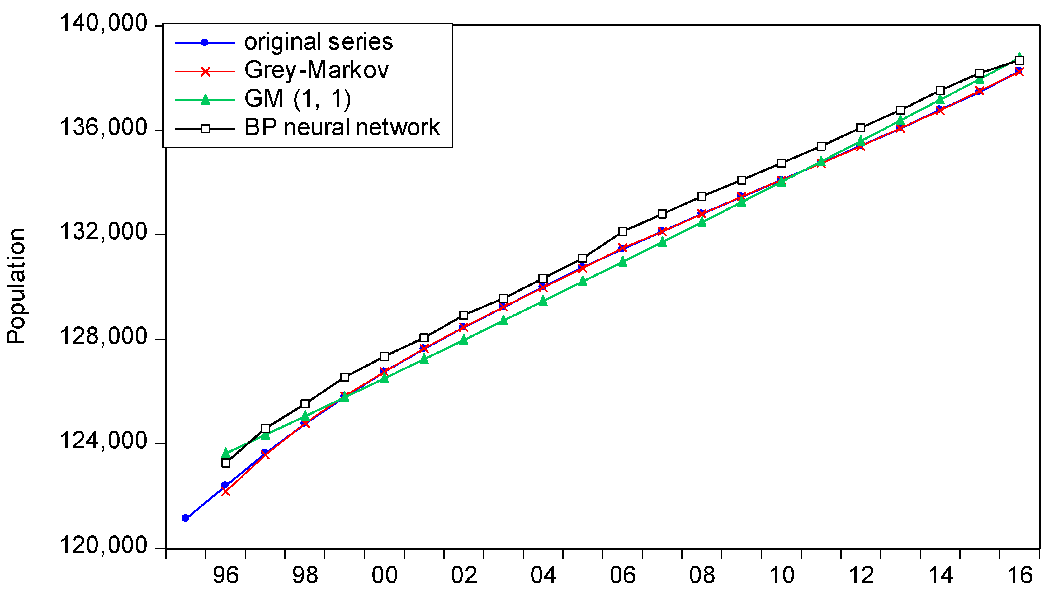
The total population has the strongest positive effect on CO₂ emissions. On one hand, population growth greatly contributes to the increase in residential electricity consumption; on the other hand, variations of population scale and enhancement of living standards have augmented the demand for products and services, which has also led to the growth of electricity consumption demand.

Line loss rate is found to be a critical factor negatively influencing the growth of CO₂ emissions of the electricity sector, and such a conclusion is consistent with [42,52]. This indicates the loss rate of electricity during the transport process has been decreasing, leading to the amount of electricity reaching the terminal to rise. Hence, CO₂ emissions in the power industry caused by line losses have been decreasing. The line loss rate declined from 8.77% in 1995 to 6.47% in 2016; however electricity production and transmission are extremely large, and losses in transmission and distribution are inevitable and cannot be ignored. For example, in 2012, aggregate electricity wastage in transmission and distribution was 289.62 TWh, greater than two year’s power use in Shanghai in terms of the current year [42]. In addition, although China has increased its technological innovation in power grid improvement, many cities have less investment in electricity-producing equipment, resulting in increased age of power transmission lines and outdated devices, and, hence, large transmission and distribution losses.

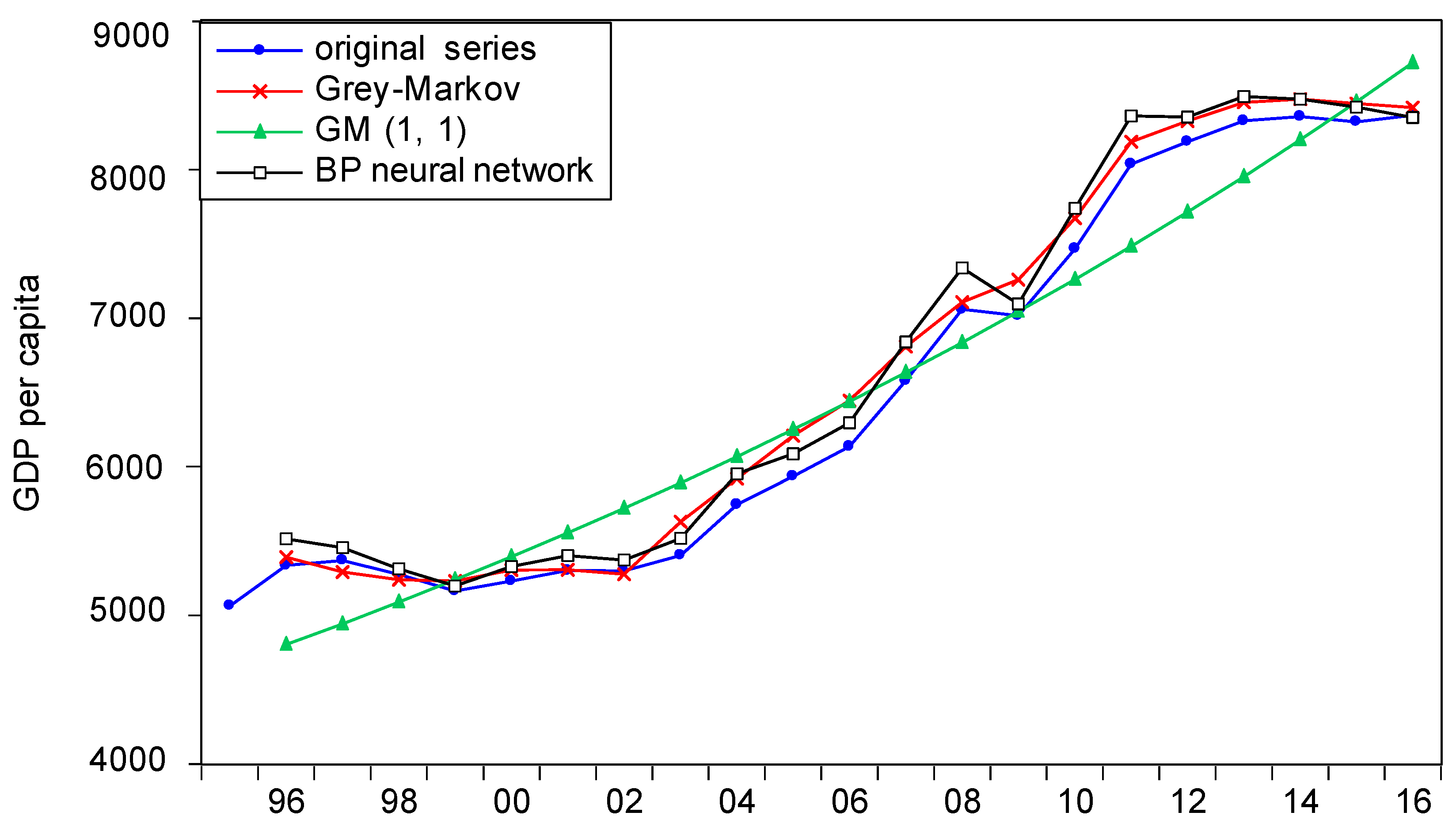
Growth in the economy is also an important contributor to CO₂ emissions of the electricity sector, accounting for a 0.669% increase in CO₂ emissions from a 1% rise in GDP per capita. GDP per capita increased from CNY 61,339.9 in 1995 to CNY 115,683.2 in 2016, the boost in which would have promoted significant development and utilization of electricity. In particular, flourishing of the economy and growth of residents’ wealth leads to increasing requirements for consumption of household appliances, which in turn leads to substantial growth in electricity consumption. The urbanization level is a relatively strong explanatory driver of CO₂ emissions. The reason for this trend is that cities are the main sources of electricity consumption in China. Along with the advancement of urbanization, the demand for electricity in urban buildings, transportation and residential buildings is also increasing. In China, the promotion of the urbanization process mainly depends on the development of secondary industry, which has intensified electricity consumption accordingly.

The indicators “generation structure” and “industrial structure”, representing the proportion of thermal power on the production side and the proportion of secondary industry on the use side, respectively, are relatively less important contributors to growth of CO₂ emissions of the electricity sector. Model results indicate a 0.522% decrease in CO₂ emissions from a 1% decrease in generation structure and a 0.060% decrease in CO₂ emissions due to a 1% decrease in industrial structure. These results are partly because economic growth in China is mostly due to construction of real estate, whose development increases the requirement for thermal power, thereby generating prominent growth in CO₂ emissions. In addition, the upgrade of secondary industry is strengthening the momentum of development; secondary industry plays a dominant role in driving growth in the short term.

Meanwhile, electricity intensity can reflect the efficiency of power consumption, but it is not one of the principal drivers of CO₂ emissions, mainly because electricity consumption per unit of GDP output was merely 16.415 kWh/CNY 10⁴ in 1995, rising to 52.080 kWh/CNY 10⁴ in 2016. Recently, China’s electricity consumption productivity has sustained an improvement because of the impact of R&D investment in energy-saving projects. Growth in the productivity of power consumption can propel electricity savings and CO₂ emission mitigation.

The PLS-Grey-Markov model can be established to perfectly fit the CO₂ emissions, compared with the other analyzed models, from 1995 to 2016. According to the forecasting model, the MAE, MAPE and RMSE values of the PLS-Grey-Markov model are lower than for other models, which shows the PLS-Grey-Markov model can effectively improve forecasting accuracy and indicates that this is a promising method for prediction of CO₂ emissions of the power sector. The hybrid model proposed offers a foundation for establishing an effectual CO₂ emission forecasting mechanism. Because of the complexity of the drivers of CO₂ emissions of the power industry, this model is mostly applicable to predicting CO₂ emissions. The feasibility of the novel forecasting method is verified above.

The PLS-Grey-Markov model has been found to perfectly predict the CO₂ emissions of the power sector. According to the forecasting model, it is expected that CO₂ emissions of the power sector in 2025 will reach 5102.925 Mt. As a result, the government and relevant departments can analyze future emission reduction measures in the power industry, to effectively adopt reasonable policies and realize low-carbon development.

6. Conclusions and Policy Implications

This paper explores drivers of CO₂ emissions of the power industry in China and obtains high-precision estimates of CO₂ emissions based on PLS and Grey-Markov models. The decomposition results indicate that the PLS model can effectually eliminate multicollinearity and illustrates that the order of emissions driving factors by absolute coefficients is: population (2.58) > line loss rate (1.112) > GDP per capita (0.669) > generation structure (0.522) > urbanization level (0.512) > electricity intensity (0.310) > industrial structure (0.060). We find that GDP per capita and total population make the strongest contributions to CO₂ emissions within the electricity sector, and that the line loss rate has a restrained impact on CO₂ emissions. The PLS-Grey-Markov model can be established to perfectly predict the CO₂ emissions of the power sector, compared with the other analyzed models, from 1995 to 2016. The forecast results indicate that CO₂ emissions of the power sector will have an increasing trend from 2017 to 2025.

These conclusions are instructive for decision-makers. Some concrete suggestions are proposed in aspects of population, technology, and the economy in order to carry out CO₂ emissions reduction and to practically implement the low-carbon development concept:

(1) Population. Population growth can greatly contribute to an increase in residential electricity consumption. It is believed that human activities will induce CO₂ emissions growth. Further, people are essential to the production process. Hence, it is crucial to achieve a balance between population growth and emissions reduction. Moreover, greater attention should be paid to improving the overall quality of population and providing motivation to implement the low-carbon concept, maintain green productivity and reduce their carbon footprints in their daily activities. Further, the urbanization rate should be rationally controlled in the urbanization process. In addition, local governments should understand the development stages and characteristics of a city, designating the future direction of urbanization. New forms of urbanization should be promoted to guarantee green electricity consumption.

(2) Technology. Environmental technology should be given top priority, playing a critical role in technological progress in the reduction of CO₂ emissions and development of a low-carbon economy. Electricity consumption productivity can be augmented by incentive policies through adopting advanced techniques, renewing power production devices and phasing out small coal-fired power enterprises. Furthermore, the investment in R&D and updating manufacturing technology should be increased in terms of fuel preparation, power plant electricity rates, and equipment amelioration. Furthermore, the implementation of ultra-low emissions and energy-saving transformations for coal-fired units and clean coal power generation technology will improve the overall quality of the power industry.

In addition, the relevant departments should pay attention to building a smart grid. Smart grid construction is a win-win technology by offering a place for both consumers and power plants to interact with the grid, improving cross-level resource scheduling. It is beneficial to enhance demand-side administration to diminish electricity consumption intensity and CO₂ emissions, and to promote consumers to adopt a low-carbon lifestyle.

(3) Economy. Relevant sectors should continue to pay attention to hastening the transformation of economic advancement. The conventional mode of large electricity usage and low efficiency production should be transformed to knowledge-intensive and technology-intensive development for attaining a more efficacious development pattern. Changing the regional economic mode mainly by raising the level of electricity delivery offers rewards, and adjustment of the industrial structure is also critical [28]. Relevant departments should not only back low-carbon enterprises, but also facilitate technology reformation to propel cleaner production and optimize the industrial structure, transforming electricity-intensive industrial sectors into more efficient ones.

At the same time, it is also critical to aspire to the coordination of development between the economy and the environment to ensure a reduction in CO₂ emissions while the economy sustains low-carbon growth. China has a strong resource commitment to renewable energy, and the acceptance of clean energy generation should also be enhanced by power grid construction. This will help the development of the local economy and also contribute to the reduction of electricity CO₂ emissions. In addition, a nation-wide carbon trading market should be established for selling certified emission reductions, to provide returns to offset the expenditure associated with low-carbon power production.

References

1. Marcucci, A.; Fragkos, P. Drivers of regional decarbonization through 2100: A multi-model decomposition analysis. Energy Econ. 2015, 51, 111–124. [Google Scholar] [CrossRef]
2. Höök, M.; Tang, X. Depletion of fossil fuels and anthropogenic climate change—A review. Energy Policy 2013, 52, 797–809. [Google Scholar] [CrossRef] [Green Version]
3. Mi, Z.F.; Zheng, J.L.; Meng, J.; Shan, Y.L.; Zheng, H.R.; Ou, J.M.; Guan, D.B.; Wei, Y.M. China’s Energy Consumption in the New Normal. Earth’s Future 2018, 6, 1007–1016. [Google Scholar] [CrossRef]
4. Cui, H.R.; Zhao, T.; Shi, H.J. STIRPAT-Based Driving Factor Decomposition Analysis of Agricultural Carbon Emissions in Hebei, China. Pol. J. Environ. Stud. 2018, 27, 1449–1461. [Google Scholar] [CrossRef] [Green Version]
5. Cui, H.R.; Wu, R.R.; Zhao, T. Dynamic Decomposition Analysis and Forecasting of Energy Consumption in Shanxi Province Based on VAR and GM (1, 1) Models. Math. Probl. Eng. 2018, 2018, 1–11. [Google Scholar] [CrossRef]
6. Meng, L.; Sager, J. Energy Consumption and Energy-Related CO2 Emissions from China’s Petrochemical Industry Based on an Environmental Input-Output Life Cycle Assessment. Energies 2017, 10, 1585. [Google Scholar] [CrossRef]
7. Sun, J.S. Research on Power Production and Bidding Model. Master’s Thesis, Jiangsu University, Nanjing, Jiangsu, China, 2016. [Google Scholar]
8. Sun, W.; Xu, Y.F. Financial security evaluation of the electric power industry in China based on a back propagation neural network optimized by genetic algorithm. Energy 2016, 101, 366–379. [Google Scholar] [CrossRef]
9. Cui, H.R.; Zhao, T.; Wu, R.R. An Investment Feasibility Analysis of CCS Retrofit Based on a Two-Stage Compound Real Options Model. Energies 2018, 11, 1711. [Google Scholar] [CrossRef]
10. Sun, W.; Wang, J.M.; Ren, Y. Research on CO2 emissions from China’s electric power industry based on system dynamics model. Int. J. Ind. Syst. Eng. 2016, 22, 423. [Google Scholar] [CrossRef]
11. Wang, W.J.; Peng, W.S.; Xu, J.M.; Zhang, R.; Zhao, Y.X. Driving Factor Analysis and Forecasting of CO2 Emissions from Power Output in China Using Scenario Analysis and CSCWOA-ELM Method. Energies 2018, 11, 2709. [Google Scholar] [CrossRef]
12. Yang, X.; Ma, C.B.; Zhang, A.L. Decomposition of Net CO2 Emission in the Wuhan Metropolitan Area of Central China. Sustainability 2016, 8, 784. [Google Scholar] [CrossRef]
13. Zha, D.L.; Zhou, D.Q.; Zhou, P. Driving forces of residential CO2 emissions in urban and rural China: An index decomposition analysis. Energy Policy 2010, 38, 3377–3383. [Google Scholar] [CrossRef]
14. Li, H.N.; Mu, H.L.; Zhang, M.; Gui, S. Sen Analysis of regional difference on impact factors of China’s energy-Related CO2 emissions. Energy 2012, 39, 319–326. [Google Scholar] [CrossRef]
15. Feng, Y.Y.; Chen, S.Q.; Zhang, L.X. System dynamics modeling for urban energy consumption and CO2 emissions: A case study of Beijing, China. Ecol. Modell. 2013, 252, 44–52. [Google Scholar] [CrossRef]
16. Wang, S.J.; Liu, X.P. China’s city-level energy-related CO2 emissions: Spatiotemporal patterns and driving forces. Appl. Energy 2017, 200, 204–214. [Google Scholar] [CrossRef]
17. Mi, Z.F.; Meng, J.; Guan, D.B.; Shan, Y.L.; Liu, Z.; Wang, Y.T.; Feng, K.S.; Wei, Y.M. Pattern changes in determinants of Chinese emissions. Environ. Res. Lett. 2017, 12, 1–10. [Google Scholar] [CrossRef]
18. Bao, G.L.; Hui, H.Q. Grey Forecasting Model for CO2 Emissions. Adv. Mater. Res. 2012, 518, 1664–1668. [Google Scholar] [CrossRef]
19. Ding, S.; Dang, Y.G.; Li, X.M.; Wang, J.J.; Zhao, K. Forecasting Chinese CO2 emissions from fuel combustion using a novel grey multivariable model. J. Clean. Prod. 2017, 162, 1527–1538. [Google Scholar] [CrossRef]
20. Zhao, H.R.; Huang, G.; Yan, N. Forecasting Energy-Related CO2 Emissions Employing a Novel SSA-LSSVM Model: Considering Structural Factors in China. Energies 2018, 11, 781. [Google Scholar] [CrossRef]
21. Dai, S.Y.; Niu, D.X.; Han, Y.R. Forecasting of Energy-Related CO2 Emissions in China Based on GM(1, 1) and Least Squares Support Vector Machine Optimized by Modified Shuffled Frog Leaping Algorithm for Sustainability. Sustainability 2018, 10, 958. [Google Scholar] [CrossRef]
22. Zhang, M.; Mu, H.; Ning, Y.; Song, Y. Decomposition of energy-related CO2 emission over 1991–2006 in China. Ecol. Econ. 2009, 68, 2122–2128. [Google Scholar] [CrossRef]
23. Wu, P.; Shi, P.H. An estimation of energy consumption and CO2 emissions in tourism sector of China. J. Geogr. Sci. 2011, 21, 733–745. [Google Scholar] [CrossRef]
24. Zhang, N.; Zhou, P.; Kung, C.C. Total-factor carbon emission performance of the Chinese transportation industry: A bootstrapped non-radial Malmquist index analysis. Renew. Sustain. Energy Rev. 2015, 41, 584–593. [Google Scholar] [CrossRef]
25. Zhao, Y.L.; Kuang, Y.Q.; Huang, N.S. Decomposition analysis in decoupling transport output from carbon emissions in Guangdong Province, China. Energies 2016, 9, 295. [Google Scholar] [CrossRef]
26. Yao, X.; Guo, C.W.; Shao, S.; Jiang, Z.J. Total-factor CO2 emission performance of China’s provincial industrial sector: A meta-frontier non-radial Malmquist index approach. Appl. Energy 2016, 184, 1142–1153. [Google Scholar] [CrossRef]
27. Zhang, C.Q.; Zhang, M.; Zhang, N. CO2 Emissions from the Power Industry in the China’s Beijing-Tianjin-Hebei Region: Decomposition and Policy Analysis. Pol. J. Environ. Stud. 2017, 26, 903–916. [Google Scholar] [CrossRef]
28. Sun, W.; Meng, M.; He, Y.J.; Chang, H. CO2 Emissions from China’s Power Industry: Scenarios and Policies for 13th Five-Year Plan. Energies 2016, 9, 825. [Google Scholar] [CrossRef]
29. Wen, L.; Yan, F.; Li, Y. Analysis of influencing factors of CO2 emissions in China’s power industry and policy implications. Pol. J. Environ. Stud. 2018, 27, 373–382. [Google Scholar] [CrossRef]
30. Zhao, W.B.; Niu, D.X. Prediction of CO2 Emission in China’s Power Generation Industry with Gauss Optimized Cuckoo Search Algorithm and Wavelet Neural Network Based on STIRPAT model with Ridge Regression. Sustainability 2017, 9, 2377. [Google Scholar] [CrossRef]
31. Lindner, S.; Liu, Z.; Guan, D.B.; Geng, Y.; Li, X. CO2 emissions from China’s power sector at the provincial level: Consumption versus production perspectives. Renew. Sustain. Energy Rev. 2013, 19, 164–172. [Google Scholar] [CrossRef]
32. Wang, H.W.; Wu, Z.B.; Meng, J. Linear and Nonlinear Methods for Partial Least Squares Regression; National Defense Industry Press: Beijing, China, 2006; ISBN 9787118044966. [Google Scholar]
33. Wang, H.W.; Huang, L. Functional Linear Regression Analysis Based on Partial Least Squares and Its Application. In The Multiple Facets of Partial Least Squares and Related Methods; Abdi, H., Esposito Vinzi, V., Russolillo, G., Saporta, G., Trinchera, L., Eds.; Springer: Cham, Switzerland, 2016; Volume 173, pp. 201–211. [Google Scholar]
34. Deng, J.L. Introduction to Grey System Theory. J. Grey Syst. 1989, 1, 1–24. [Google Scholar]
35. He, Y.D.; Bao, Y.D. Grey-Markov forecasting model and its application. Syst. Eng. Pract. 1992, 9, 59–63. [Google Scholar]
36. Kumar, U.; Jain, V.K. Time series models (Grey-Markov, Grey Model with rolling mechanism and singular spectrum analysis) to forecast energy consumption in India. Energy 2010, 35, 1709–1716. [Google Scholar] [CrossRef]
37. Ehrlich, P.R.; Holdren, J.P. Impact of population growth. Science 1971, 171, 1212. [Google Scholar] [CrossRef] [PubMed]
38. Yang, L.X.; Xia, H.; Zhang, X.L.; Yuan, S.F. What matters for carbon emissions in regional sectors? A China study of extended STIRPAT model. J. Clean. Prod. 2018, 180, 595–602. [Google Scholar] [CrossRef]
39. Dietz, T.; Rosa, E.A. Rethinking the environmental impacts of population, affluence and technology. Hum. Ecol. Rev. 1994, 1, 277–300. [Google Scholar]
40. Soule, P.T.; Dehart, J.L. Assessing IPAT Using Production- and Consumption-based Measures of I. Soc. Sci. Q. 1998, 79, 754–765. [Google Scholar]
41. Zhang, C.Q.; Zhang, M.; Zhang, N. Identifying the Determinants of CO2 Emission Change in China’s Power Sector. Discret. Dyn. Nat. Soc. 2016, 2016, 1–12. [Google Scholar] [CrossRef]
42. Yan, D.; Lei, Y.L.; Li, L. Driving Factor Analysis of Carbon Emissions in China’s Power Sector for Low-Carbon Economy. Math. Probl. Eng. 2017, 2017. [Google Scholar] [CrossRef]
43. Wang, P.; Wu, W.S.; Zhu, B.Z.; Wei, Y.M. Examining the impact factors of energy-related CO2 emissions using the STIRPAT model in Guangdong Province, China. Appl. Energy 2015, 106, 65–71. [Google Scholar] [CrossRef]
44. Noorpoor, A.R.; Kudahi, S.N. CO2 emissions from Iran’s power sector and analysis of the influencing factors using the stochastic impacts by regression on population, affluence and technology (STIRPAT) model. Carbon Manag. 2015, 6, 101–116. [Google Scholar] [CrossRef]
45. Agency, I.E. IPCC guidelines for National Greenhouse Gas Inventories. Energy 2006, 2, 52–57. [Google Scholar] [CrossRef]
46. Wang, C.J.; Wang, F.; Su, Y.X.; Ye, Y.Y. Examining the driving factors of energy related carbon emissions using the extended STIRPAT model based on IPAT identity in Xinjiang. Renew. Sustain. Energy Rev. 2017, 67, 51–61. [Google Scholar] [CrossRef]
47. National Bureau of Statistics. China Statistical Yearbook of 2017; China Statistics Press: Beijing, China, 2017; ISBN 978-7-5037-8253-4. [Google Scholar]
48. Editorial Committee of China Electric Power Yearbook. China Electric Yearbook-2017; China Electric Power Press: Beijing, China, 2018; ISBN 9787519815066. [Google Scholar]
49. China Electricity Council National Electric Power Industry Statistics Express 2017. Available online: http://www.cec.org.cn/guihuayutongji/tongjxinxi/yuedushuju/2017-12-19/176259.html (accessed on 19 March 2018).
50. Jia, J.P.; He, X.Q.; Jin, Y.J. Statistics; China Renmin University Press: Beijing, China, 2004; ISBN 7-300-03589-2. [Google Scholar]
51. Yang, H.R. Research and Implementation on Water Quality Multi-Parameter Monitoring Using PLS Method. Master’s Thesis, University of Electronic Science and Technology of China, Chengdu, Sichuan, China, 2009. [Google Scholar]
52. Cui, H.R.; Zhao, T.; Wu, R.R. CO2 emissions from China’s power industry: Policy implications from both macro and micro perspectives. J. Clean. Prod. 2018, 200, 746–755. [Google Scholar] [CrossRef]
Figure 1. Growth of CO2 emissions in the power sector.
Energies 11 02985 g001
Figure 2. The forecasting results for population.
Energies 11 02985 g002
Figure 3. The forecasting results for GDP per capita.
Energies 11 02985 g003
Figure 4. The forecasting results for industrial structure.
Energies 11 02985 g004
Figure 5. The forecasting results for industrial structure.
Energies 11 02985 g005
Figure 6. The forecasting results for electricity intensity.
Energies 11 02985 g006
Figure 7. The forecasting results for line loss rate.
Energies 11 02985 g007
Figure 8. The forecasting results for urbanization level.
Energies 11 02985 g008
Figure 9. The forecasting result for CO2 emissions in the electricity generation sector by the PLS-Grey-Markov model from 1995 to 2016.
Energies 11 02985 g009
Figure 10. The forecasting result of CO2 emissions in the power generation sector from 2017 to 2025.
Energies 11 02985 g010