Article

Prediction of Remaining Useful Life of Wind Turbine Bearings under Non-Stationary Operating Conditions

1
School of Instrumentation and Optoelectronic Engineering, Beihang University, Beijing 100083, China
2
Department of Electrical and Computer Engineering, University of Calgary, 2500 University Dr NW, Calgary, AB T2N 1N4, Canada
3
Department of Mechanical and Manufacturing Engineering, University of Calgary, 2500 University Dr NW, Calgary, AB T2N 1N4, Canada
*
Author to whom correspondence should be addressed.
Submission received: 5 November 2018 / Revised: 22 November 2018 / Accepted: 23 November 2018 / Published: 28 November 2018
(This article belongs to the Section A: Sustainable Energy)

Abstract

:
Wind-powered electricity generation has grown significantly over the past decade. While there are many components that might impact their useful life, the gearbox and generator bearings are among the most fragile components in wind turbines. Therefore, the prediction of remaining useful life (RUL) of faulty or damaged wind turbine bearings will provide useful support for reliability evaluation and advanced maintenance of wind turbines. This paper proposes a data-driven method combining the interval whitenization method with a Gaussian process (GP) algorithm in order to predict the RUL of wind turbine generator bearings. Firstly, a wavelet packet transform is used to eliminate noise in the vibration signals and extract the characteristic fault signals. A comprehensive analysis of the real degradation process is used to determine the indicators of degradation. The interval whitenization method is proposed to reduce the interference of non-stationary operating conditions to improve the quality of health indicators. Finally, the GP method is utilized to construct the model which reflects the relationship between the RUL and health indicators. The method is assessed using actual vibration datasets from two wind turbines. The prediction results demonstrate that the proposed method can reduce the effect of non-stationary operating conditions. In addition, compared with the support vector regression (SVR) method and artificial neural network (ANN), the prediction accuracy of the proposed method has an improvement of more than 65.8%. The prediction results verify the effectiveness and superiority of the proposed method.

1. Introduction

Wind energy as a renewable energy is growing rapidly around the world. However, the operation and maintenance (O&M) costs caused by the premature failure of the main components of wind turbine generator can account for 10–20% of the total energy cost for a wind turbine project [1,2]. Bearings, a fundamental component of wind turbine gearboxes and generators, are among the most fragile components of wind turbines [3,4]. Damages in bearings can cause a high impact on economic cost and reliability of wind turbines [3,4,5]. For example, bearings cause more than 50% of the faults on gearboxes, leading to the growth of maintenance costs for turbine owners and operators [3,4]. Moreover, early cracks in bearings have been detected with less than 5–10% of the expected life, that is, within 3 years of operation [3]. Thus, efficient techniques of condition monitoring and remaining useful life (RUL) prediction of wind turbine bearing is an important issue. Several analyses of bearing fault diagnostics and condition monitoring have been reported [6,7,8] as have studies of the remaining useful lifetime (RUL) of wind turbine bearings [1,9,10,11,12,13]. Such RUL predictions have the potential to reduce downtime cost and to support proactive maintenance scheduling [14,15] that can lengthen service life.
The RUL prediction methods can be broadly classified into model-based methods, and data-driven methods [16]. The model-based methods attempt to construct physical or mathematical degradation models to predict the RUL of a machine [17]. Lei et al. [18] proposed a model-based method with two modules, combined with a particle filtering (PF) algorithm based on the vibration data from the PRONOSTIA experiment system. Djeziri et al. [16] introduced a hybrid method, which included a physical model, clustering algorithm and the Euclidean distance to predict the RUL of the wind turbine bearing simulator. Saidi et al. [19] proposed an integrated prognostics method to predict the RUL of wind turbine high-speed shaft bearings, which combined physical degradation models and data-driven approaches. Lei et al. [20] used a new stochastic process model and the Kalman particle filtering algorithm for RUL prediction. The effectiveness of model-based methods depends on the accuracy of the model, which is difficult to determine and may be specific to one bearing type. Model-based methods also have a limited capability to include detailed information about the fault that might be available [17].
Data-driven methods are more popular in the literature. For example, Teng et al. [10] proposed a method which combined an artificial neural network (ANN) with a polynomial fitting curve to predict the RUL of an operating wind turbine. Saidi et al. [13] proposed a spectral kurtosis data-driven approach to predict the RUL of wind turbine high-speed shaft bearing, which combined a new condition indicator and SVR method. Zhou et al. [11] used an adaptive neuro-fuzzy inference system and PF to analyse the current signals of the simulator to predict the RUL. Data-driven methods, however, face some challenges. One challenge is to construct suitable health indicators to reflect the degradation of the bearing. In some studies, non-vibration signals were used to construct health indicators. For example, Gong et al. [21] used generator current signals for this purpose. Rodney et al. [22] used current and vibration data to select health indicators in order to estimate the bearing RUL. As the vibration signals are a rich source of failure information, the vibration signals are used in most of the RUL prediction research. Moreover, in order to construct suitable health indicators to improve the prediction effect, multiple features have been selected by considering the monotonicity and tendency of features [23,24,25,26]. Lei et al. [18] constructed a new health indicator named weighted minimum quantization error, which fused mutual information from multiple features. In summary, while significant works are presented on health indicator extraction and selection, there is little emphasis on the real degradation process of the bearing during operation. The present paper selects characteristic features as the health indicators by analysing the degradation trend to improve the prediction effect, instead of only considering the monotonicity and tendency of characteristic features.
Another challenge of the data-driven methods is on how to deal with non-stationary operating conditions, which are typical of modern wind turbines. Most research on RUL prediction used experimental or simulated data for stationary conditions, i.e., constant speed, constant load, etc. However, in general, wind turbines operate in variable speed and load conditions, which leads to a large fluctuation in the health indicators [27]. There are other time-frequency analysis methods for non-stationary signals, such as angle analysis and order tracking analysis [28,29]. An accurate rotational speed measurement is critical for these methods. There are two main ways to get accurate rotational speed, i.e., measurement via a tachometer and indirect estimation based on vibration analysis. The measurement of rotating speed via a tachometer may lead to sampling loss and unacceptable errors when the rotating speed changes rapidly [28,30]. Thus, several studies are developed for indirect estimations of rotational speed based on vibration analysis, especially the estimation of instantaneous frequency (IF) [31]. An example is the time–frequency distribution (TFD) methods. The IF estimation based on moments of TFD is limited in analyses of practical multi-components signals because it has physical meaning only for mono-component signals. The IF estimation on the basis of peaks of TFD is also restricted to the time and frequency resolution. Thus, these methods required high time-frequency resolution to ensure precision [28]. Moreover, the synchronization between a new accelerometer and the existing turbine SCADA system and monitoring equipment may require retrofitting. Compared with such methods, the interval whitenization (IW) method has the characteristics of generality, less calculation, and is independent of the rotational speed and is less sensitive to time-frequency resolution. In this paper, the IW method is used for the first time to reduce the interference of non-stationary operating conditions.
Thus, the main contribution of this paper is to propose an interval whitenization Gaussian process (IWGP) prediction method, which combines the IW method with a Gaussian process (GP) prediction algorithm for RUL prediction. In the proposed method, the health indicators are selected to reflect the degradation process through analysing the relationship between fault characteristics and the fault severity. Furthermore, the IW method is used for the first time to reduce the fluctuation of health indicators caused by non-stationary operation. The GP method is used to build the RUL prediction model. The advantage of using the IW method is that it can deal with uncertain information in a system, Here, the complex operating conditions are uncertain information for the condition monitoring system. Thus, the IW method is chosen to reduce the effect of non-stationary operating conditions for the RUL prediction. Additionally, compared with traditional methods, such as artificial neural networks (ANNs), or support vector machine regression (SVR), the GP method has the advantages in being probabilistic and nonparametric. Furthermore, the GP method is able to handle small sample datasets, and deal with nonlinear and non-stationary problems [31], both of which important for this application.
The rest of the paper is organized as follows. Section 2 presents the basic theory of GP. Section 3 shows the proposed prediction method. In Section 4, the proposed prediction method is demonstrated using real-world datasets of two turbines from a wind farm. Conclusions are presented in Section 5.

2. The Basic Theory of Gaussian Process

The Gaussian process is a practical probabilistic kernel machine learning approach and has been applied in many machine learning tasks due to its advantage of being flexible, probabilistic, and nonparametric [31,32,33,34,35,36]. GP regression was used in Reference [37] for reserve estimation of a photovoltaic system. The GP method combined with a numerical weather prediction model was used for wind speed prediction up to 72 h ahead in Reference [38]. The GP method performed better than ANN and support vector machine (SVM) in tool wear prediction in Reference [39]. In this paper, the GP method is used in RUL prediction of wind turbine bearings. The behaviour of any system can be modelled through combining the Gaussian Process with prior knowledge based on the Bayesian framework. In this section, a high-level description of the GP method is provided. A detailed outline of this method can be found in the literature (e.g., References [40,41]). The GP model assumes that the output is a realisation of a GP with joint probability density function f ( x ) ~ GP   ( m ,   k ) , where,
m i = m ( x i ) = E ( f ( x i ) )
k i j = k ( x i , x j ) = E [ ( f ( x i ) m i ) ( f ( x j ) m j ) ]
where k ( x i , x j ) , ( i , j = 1 , , N ) is the covariance function or kernel. Usually, the mean function is assumed to be zero, and the mean of the target variable is normalized to zero [41].
The GP method can be applied to a classical regression problem as follows. Assume X = [ x 1 , x 2 , , x N ] represents N, D-dimensional input vectors, and the corresponding outputs are y = [ y 1 , y 2 , , y N ] T new input vector x is given and the aim is to predict the corresponding output y Consider the static relationship
y i = φ ( x i ; w ) + ε ,   ε ~ N ( 0 , σ n 2 ) ,   i = 1 ,   ,   N
where φ is a function parameterized by the vector w ; ε is assumed to be the noise caused by stochastic disturbances or distributed Gaussian distribution N with zero mean and variance σ n 2 .
The prior probability on y is:
E [ y ] = E [ φ ( x ;   w ) + ε ] = 0
cov [ y ] = K ( X , X ) + σ n 2 I
where E is the mean function, cov is the variance function.
The distribution with the new input can be expressed by the function,
[ y y ] ~ G P ( 0 , [ K ( X , X ) + σ n 2 I K ( X , x ) K ( X , x ) T K ( x , x ) ] )
where K ( X , x ) = [ k ( x 1 , x ) , ,   k ( x N , x ) ] can be shortened to k . According to the theory of joint Gaussian distributions, the prediction results can be presented by the following:
E ( y ) = k T ( K + σ n 2 I ) 1 k T
cov [ y ] = k ( x , x ) k T ( K + σ n 2 I ) 1 k

3. The Proposed RUL Prediction Method

The block diagram of the IWGP method is shown in Figure 1. Briefly, the wavelet packet transform (WPT) is used to pre-process the raw vibration signals to reduce noise and the raw health indicators are extracted by considering the real degradation process; this is done by analysing the amplitude spectrums in different fault levels and summarizing the variation characteristic of amplitude with the degradation process. Then, the IW method is applied to the raw health indicators to reduce the fluctuations caused by non-stationary operation. After that, the GP method is used to build the RUL prediction model, taking the whitened health indicators as the model inputs and the RUL as the model output. Further details of the proposed method are provided next.

3.1. Health Indicators Extraction

The health indicator extraction process is particularly important to the accuracy of the RUL prediction. The faults of the bearing are located in the rolling element, the inner race, or the outer race. Faulty bearings typically generate distinct frequencies: the ball pass inner race (BPFI), the fundamental train frequency (FTF), the ball spin frequency (BSF), the ball pass outer race (BPFO). The faults can be detected by the impulse events at the characteristic frequencies [42]. However, as the rotational speed and load change, the location and amplitude of fault characteristic frequencies vary with the operational speed. Furthermore, vibration signals may be disturbed by noise in a harsh working environment as well as noise from other rotating components in the drive-train. Therefore, it is very important to extract the characteristic frequency signal accurately.
The WPT method has been widely applied to decompose signals and extract characteristic features [43,44,45]. The WPT method was used to extract features from on-line cutting force signals for the real-time monitoring of surface roughness in automated manufacturing systems [43]. In Reference [45], the WPT combined with the manifold learning method was used to extract the weak signals for the rolling bearing fault diagnosis. In Reference [45], the wavelets transform method was employed to filter and diagnosis the ice condition on the wind turbine blade surface. In this paper, the WPT method is used to de-noise and extract the developed health indicators.
For outer race bearings, the faults can be identified by the magnitude of the characteristic frequencies, and the theoretical fault characteristic frequencies can be calculated [46]. If the shaft speed is within a certain range, the characteristic frequencies and its harmonics will have a minimum limit value Fmin and a maximum limit value Fmax. Fmin is the minimum value of the harmonic frequency at the lowest rotational speed, and Fmax is the maximum value of the harmonic frequency at the highest rotational speed. Thus, the health indicators can be extracted using the characteristic signal within this frequency range [Fmin, Fmax]. The influence of noise can be reduced by using the WPT method.
As time passes, the fault severity of the bearings increases. In this paper, the suitable health indicators are constructed to reflect degradation tendency by analysing the degradation process. Figure 2 shows amplitude spectra in different months of a wind turbine generator bearing (WTGB) from one of the wind turbines for which we collected data—we refer to it as wind turbine #1 in this paper. Further details on the wind turbine and the collected datasets can be found in Section 4. In Figure 2, the degradation tendency is observed as time goes on, and the fault severity increases, the amplitude of fault characteristic frequencies increases and the frequency ranges including the fault characteristic frequency bands become wider. The variance of amplitude represents the variance of energy. Energy entropy (EE), a time-frequency feature, represents the uncertainty of the energy distribution in different frequency bands. The EE value decreases first and then increases as the fault severity increases. The RMS value represents the energy of the characteristic signal that changes as the degradation process. Thus, these two features can be used to represent the tendency of fault development in the RUL prediction.
The energy entropy H is defined as
E N [ m , n ] = Σ t = 1 N     W [ m , n ] 2 ( t )
P [ m , n ] = E [ m , n ] n = 0 2 m 1 E [ m , n ]
H = Σ n = 0 2 m 1     P [ m , n ] ln P [ m , n ]
where, N represents the length of the reconstructed signal by the WPT method; W [ m , n ] ( t ) is the reconstructed signal of the WPT terminal node; E N [ m , n ] is the energy of the reconstructed signal and P [ m , n ] is the energy distribution of each node.
The root mean square (RMS) value is defined as
RMS = 1 N Σ t = 1 N W [ 0 , 0 ] 2 ( t )
where W [ 0 , 0 ] ( t ) is the reconstructed signal after setting the wavelet terminal coefficients outside the frequency range to zero [Fmin, Fmax].
The health indicators extracted from the vibration signal of WTGB are not only influenced by the fault severity, but also influenced by the non-stationary operating conditions. As the shaft speed is measured by the turbine supervisory control and data acquisition (SCADA) system, whereas bearing vibration may be measured separately, combining the data and determining the extract operating conditions may be difficult. Thus the health indicators are uncertain and fluctuate. In this paper, the IW method is used for the first time to reduce the fluctuation of health indicators caused by the non-stationary operating conditions, which can improve the accuracy of RUL prediction.

3.2. Interval Whitenization (IW) Method

In system theory, a system can be defined with a colour that represents the severity of clear information of the system. For instance, a “black” system is completely unknown. On the contrary, if the system is completely known, it is a “white” system. A system somewhere in between is called a “grey” system. In reality, every system can be modelled as a grey system because of uncertain factors, such as noise, external causes and the limitation of our cognitive ability. Therefore, a condition monitoring system can be modelled as a grey system if the operating conditions are not known. The interval whitenization method has been applied in grey systems to deal with uncertain information and has demonstrated to be one of the best algorithms to improve the prediction accuracy. A systematic description of the IW method is given in Reference [47].
The fluctuation range of a data sequence within a short period of measurement time (SPMT) i can be expressed as an interval with a lower bound and an upper bound, denoted by W i = [ a i , b i ] . Where a i < b i . An example of a fluctuating health indicator from wind turbine #1 is shown in Figure 3, where the envelopes of lower and upper bounds change with time and possibly indicate the changing trends of the fault severity. Since the health indicator in the interval W i is uncertain, a probable value is required to represent it, which is that a proper value of health indicator is determined to represent the current fault severity. The probable value is called the interval grey number in a grey system [47]. A triangular whitenization weight function is one of the most common functions for describing the probable degree of a grey number in the interval, which is shown in Figure 4. If a o = b o , the expectation of the whitenization weight function, represented by ‘o’, is the centre of W .
During a longer condition monitoring time, the fluctuating health indicator data sequence can be denoted as X = ( W 1 , W 2 , , W n ) , where n is the number of SPMTs. W i = [ a i , b i ]   ( i = 1 , , n ) is the fluctuation range of the probability density function (PDF) in the i - t h SPMT, as shown in Figure 5. The lower bound a i and upper bound b i have the same changing trends. As the wind speed is stochastic, so it is assumed that the health indicator value in W i obeys a uniform distribution. Applying the whitenization weight function to the data in each SPMT and setting a o = b o , the proper value can be obtained, shown in Figure 5, where, o i represents the proper value in the i - t h SPMT. After applying the IW method to the data sequence X , the fluctuation range in each SPMT is represented by a proper value, and the tendency retains due to the fault severity.
A vibration dataset of a normal WTGB is used to test the effectiveness of the proposed IW method, which can reduce the effect of the non-stationary operating condition. The extracted raw RMS value is expressed in blue dotted lines and processed RMS value by IW method with two days as an SPMT is expressed in the red line in Figure 6.
The large fluctuation of the RMS values is shown in Figure 6. These fluctuations may be mainly caused by noise and non-stationary operating conditions. Compared with the raw data shown as the blue line, the processed data shown in the red line has fewer fluctuations. Therefore, the IW method can reduce the fluctuation of health indicators caused by non-stationary operating conditions to improve the prediction effect.
There are a number of prognostic techniques for the non-linear and non-stationary process [31], such as match matrix (MM), particle filtering (PF), extend Kalman filtering (EKF) or order tracking analysis. All these can deal with non-stationary processes. However, the MM method is time-consuming to apply, has a low efficiency, and needs large amounts of historical data [48]. The PF method suffers from computation and storage problems [20,49]. The EKF method commonly applies to system identification and state estimation, however, it usually performs poorly for approximately non-Gaussian processes [50]. The order tracking analysis has become widely used recently, but accurate rotational speed is critical for these methods, and higher time-frequency resolution is required. Compared with the above methods, the IW method has the advantage of fast computation, generality, is independent of the rotational speed, and is less sensitive to time-frequency resolution. It is available for small sample data with the appropriate weight function and SPMT for non-linear and non-stationary processes. Thus, the IW is used in this paper to reduce the effect of non-stationary operating condition.

3.3. RUL Prediction

The GP prediction method has been applied successfully in many domains, both in regression and classification, particularly when there is a limited amount of data available. In this work, because of limited real wind turbine bearing data and the non-linear, non-stationary degradation process, the GP prediction method is utilized to predict the RUL of the WTGB.
In this paper, the raw vibration signals are pre-processed by the WPT method to reduce noise and extract raw health indicators. Here, by analysing the relationship between assumed fault characteristic features and the assumed fault severity, i.e., summarizing the characteristic from the amplitude spectrums with different fault levels, the RMS and EE values are selected as the health indicators to reflect the degradation process. Then, the raw health indicators are processed to reduce the effect of non-stationary operating conditions by IW method. The processed health indicators are called WI health indicators. The GP method is used to construct the prediction module. In the module, the WI health indicators are as the input, and the RUL (in days) is the output. In this paper, the datasets of one wind turbine are used to train the module, and another wind turbine is used to validate the effectiveness of the proposed method.

4. Experimental Validation

In this section, the IWGP method is applied to the WTGB online condition monitoring data. Two datasets are used to evaluate the method from two wind turbines.

4.1. Data Introduction

In this paper, the actual vibration signals of two wind turbines are used to test the effect of the proposed method. The turbines are from the Tong Fa wind farm in Jilin Province, North-eastern China. The vibration signals are collected by accelerometers through the vibration on-line condition monitor what shown in Figure 7. The accelerometer was vertically mounted on the generator bearing in Figure 7c. As shown in Figure 8, eight accelerometers were installed on the drive train of a wind turbine. The A7and A8 accelerometers mounted on generator front and rear bearings. In this paper, the vibration datasets of the A8 accelerometer, are used to predict the RUL of generator bearing. The sampling frequency is 2500 Hz. These datasets include two vibration datasets that span from the normal, assumed fault-free operation to the final fault alarm. These two bearings were both checked after the fault alarm. They both had extensive electric erosion and had to be replaced. The datasets of wind turbine #1 are used to train the RUL prediction model and the other is used as a test set. The detailed information of the data is shown in Table 1.
The generator starts producing power at a rotational speed of 1100 rpm for the initial power generation and reaches the rated power (850 kW) at the maximum rotational speed of 1680 rpm. These speeds were used to determine the frequency range of bearing faults in Table 2.

4.2. The Effectiveness of the Proposed Model

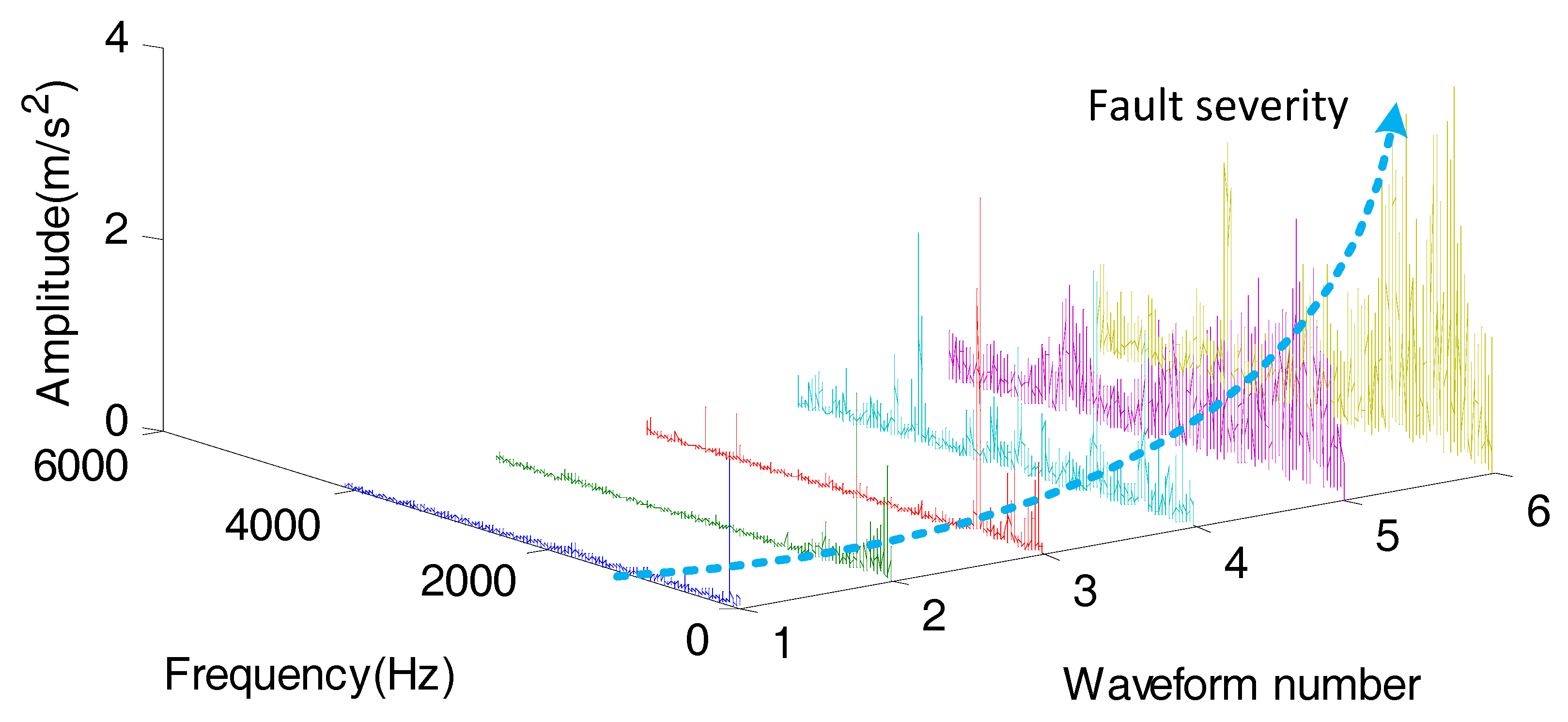
4.2.1. The Effectiveness of the Health Indicators

The fault characteristic frequencies of the bearing are calculated and shown in Table 2 [46]. Here, f r is the rotational frequency.
The discrete Meyer wavelet has been previously used to accurately extract the characteristic signal in the bearing vibration signals [51]. In Figure 9, there are different reconstruction signals with different basic functions. Compared with the results based on several common basis functions, the Meyer function performs well in extracting the characteristic signal; some interference would appear in the reconstructed signal using other basic functions. Thus, the Meyer function is selected as the basic function of WPT. Considering the characteristic frequency range and the sampling frequency, the vibration data have been decomposed into five levels. The energies of the terminal nodes are as shown in Figure 10. In Figure 10, the waveform numbers represent the vibration signals in six months from wind turbine #1. In Table 3, the mean energy ratio value of nodes 0 to 14 of 6 signals represents more than 80% of the total energy. Therefore, the terminal nodes 0 to 14 are chosen to reconstruct the signal. The reconstructed signal is obtained by setting other wavelet terminal coefficients to zero, which is shown in Figure 11. The influence of noise can be eliminated by pre-processing while retaining the characteristic signals by the WPT method. According to Section 3.1 the RMS and EE values are extracted as the health indicators from the de-noised signals.
As an alternative to the WPT method, the empirical mode decomposition (EMD) method is a self-adaptive signal processing technique and is widely used [52]. We also implemented the EMD method to de-noise the raw signal, as summarized in Figure 12. In the EMD method, the intrinsic mode functions (IMFs) with a high correlation coefficient (>0.1) are selected. As Figure 13 shows, the first seven IMFs are used to construct signals. The constructed signals by the EMD method is expected to retain the main information of the raw signals and eliminate the noise.
The frequency spectrums of the signals by the EMD and WPT methods are shown in Figure 14. Compared with the WPT method, the reconstructed EMD signals have more spectral content in both low and high frequencies which is irrelevant for the fault detection. Therefore, the WPT method is used to de-noise and extract health indicators in this paper.

4.2.2. The Effectiveness of the IW Method

According to wind farm operators, a WTGB with a fault in the bearing may continue to operate. Assuming that the bearings are initially healthy, during SPMT, the fault severity will develop very slowly. Thus, it is thought that the variation of health indicators only results from a change in operating conditions. Here, as the fault is caused by electrical corrosion, the two days are taken as SPMT.
As in the previous subsection, the RMS and the EE values are the health indicators after WPT decomposition, and then the health indicators are processed by the IW method. As shown in Figure 15, the whitened health indicators (processed health indicators by the IW method) are denoted with ‘*’, and the raw health indicators are denoted with ‘·’. Since the whitened health indicators have a smaller variation than the raw health indicators, the IW method can be used to reduce the fluctuation level. The fluctuations of the health indicators are reduced and the tendency is retained. Thus, the IW method is effective in reducing the interference of non-stationary operating condition.

4.2.3. The Effectiveness of the Prediction Model

The wind turbine downtime starts with the fault and continues with the logistic time to prepare parts and equipment, the time to wait for good weather, the time to travel/access to the site, and the actual repair and dispatch time. According to the statistics, most of the wind turbine downtimes is 10 days to 20 days [53]. In this paper, the failure is in generator bearing. According to Reference [53], the two wind turbines downtime (i.e., maintenance process) can be calculated for approximately 12 days. Here, considering practical complexities and logistics, a safe total preparation time t s = 20 days is a practical value for the wind farm operators to bring the turbine back to work after a bearing fault.
The dataset of wind turbine #1 is used for training the model and the other wind turbine dataset is used for testing. The GP method is used to construct the model. The health indicators are the model input, the corresponding RUL (days to the end life) is as the model output.
The prediction result is shown in Figure 16. The blue line represents the actual RUL, the red line represents the prediction result by the IWGP method. As Figure 16 shows, the IWGP gives an accurate prediction, especially in the late stage of the bearing life. Moreover, when the actual RUL reaches t s , the estimated RUL by IWGP is 16.7 days, so the predicting accuracy is ( 20 16.7 ) / 20 = 16.5 % . In practical applications, it is sufficient to make an effective maintenance schedule. Note that the cost of repair, which is partly that of getting a large crane to the site, means that the value of RUL is most often the ability to schedule the maintenance of the maximum number of wind turbines at the same time.
Figure 17 shows the prediction results with different methods in the late stage of the bearing life based on WI health indicators. The health indicators processed by the IW method are called the WI health indicators. In this figure, the blue line is the actual RUL, the purple line represents the prediction result by the IW method and SVR method, the green line represents the result by the IW method and BP method, the red line represents the result of the IWGP method. As Figure 17 shows, the prediction effect of IWGP is better than the other methods in the late stage. Moreover, when the real RUL reaches t s , the prediction results of IW-BP and IW-SVR are 50.8 and 29.6 days respectively. Obviously, the prediction effect of BP is poor. The prediction error of the SVR method is up to |20 − 29.6|/20 = 48.2%. Thus, compared with the two methods, the IWGP method gives better predictions.
The prediction results that the IW method does not use are shown in Figure 18. Compared with Figure 17, a great improvement in the prediction accuracy is seen after applying the IW method. The IW method can reduce the effect of non-stationary operating conditions, moreover improving the prediction accuracy.

5. Conclusions

In this paper, the IWGP method is proposed for the RUL prediction of bearing under non-stationary operating conditions. The health indicators are selected through correlating with the degradation process. It is the first time that the IW method is used to eliminate the effect of non-stationary operating conditions. The RUL is predicted using the GP method.
Two wind turbine generator bearing vibration datasets are used to validate the effectiveness of the proposed method. The prediction results demonstrate that the prediction accuracy of the IWGP method is 16.5%, compared with 48.2% of the SVR method and 154% of BP method, which has an improvement of more than 65.8%. The proposed method has a better effect on WTGB RUL prediction. From the aspect of an actual wind turbine operation and maintenance situation, 20 days is selected as a safe preparation time. The prediction results show acceptable accuracy to make an effective maintenance.
However, there are still some limitations to the proposed method. First, in terms of data, the detail information of the fault (e.g., fault location, fault type) is not available to us. Having that information could have improved that method. The other limitation is that the sampling frequency is low because the more fault information would be extracted and the prediction effect would be better based on high sampling frequency data. Moreover, the SPTM of the IW method is chosen to just rely on the statistical data of a wind farm. Therefore, further work is needed to validate the proposed method based on more datasets (high sampling frequency and complete fault information), and optimize the choice of SPTM to improve the prediction accuracy. These are the future works of the authors.

Author Contributions

Methodology, L.C.; writing—original draft, L.C., Z.Q. and S.T.; draft—review and editing, Z.Q., H.Z., D.W., E.M. and P.Y.

Funding

This research was funded by the National Nature Science Foundation of China grant number [61573046].

Conflicts of Interest

The authors declare no conflict of interest.

Abbreviations

RULremaining useful life
O&Moperation and maintenance
PFparticle filtering
ANNartificial neural network
IFinstantaneous frequency
TFDtime frequency distribution
SCADAsupervisory control and data acquisition
IWGPinterval whitenization and gaussian process
IWinterval whitenization
GPgaussian process
SVRsupport vector regression
SVMsupport vector machine
WPTwavelet packet transform
BPFIball pass inner race
FTFfundamental train frequency
BSFball spin frequency
BPFOball pass outer race
WTGBwind turbine generator bearing
RMSroot mean square
EEenergy entropy
SPMTshort period of measurement time
PDFprobability density function
MMmatch matrix
EKFextend kalman filtering
EMDempirical mode decomposition
IMFintrinsic mode function

References

  1. Hu, Y.; Li, H.; Shi, P.; Chai, Z.; Wang, K.; Xie, X.; Chen, Z. A prediction method for the real-time remaining useful life of wind turbine bearings based on the wiener process. Renew. Energy 2018, 127, 452–460. [Google Scholar] [CrossRef]
  2. Peeters, C.; Guillaume, P.; Helsen, J. Vibration-based bearing fault detection for operations and maintenance cost reduction in wind energy. Renew. Energy 2018, 116, 74–87. [Google Scholar] [CrossRef]
  3. de Azevedo, H.D.M.; Araújo, A.M.; Bouchonneau, N. A review of wind turbine bearing condition monitoring: State of the art and challenges. Renew. Sustain. Energy Rev. 2016, 56, 368–379. [Google Scholar] [CrossRef]
  4. Sheng, S. Wind Turbine Gearbox Reliability Database, Condition Monitoring, and O&M Research Update; National Renewable Energy Laboratory (NREL): Golden, CO, USA, 2016.
  5. Lin, Y.; Tu, L.; Liu, H.; Li, W. Fault analysis of wind turbines in china. Renew. Sustain. Energy Rev. 2016, 55, 482–490. [Google Scholar] [CrossRef]
  6. Gao, Q.W.; Liu, W.Y.; Tang, B.P.; Li, G.J. A novel wind turbine fault diagnosis method based on intergral extension load mean decomposition multiscale entropy and least squares support vector machine. Renew. Energy 2018, 116, 169–175. [Google Scholar] [CrossRef]
  7. Chen, J.; Pan, J.; Li, Z.; Zi, Y.; Chen, X. Generator bearing fault diagnosis for wind turbine via empirical wavelet transform using measured vibration signals. Renew. Energy 2016, 89, 80–92. [Google Scholar] [CrossRef]
  8. Yang, D.; Li, H.; Hu, Y.; Zhao, J.; Xiao, H.; Lan, Y. Vibration condition monitoring system for wind turbine bearings based on noise suppression with multi-point data fusion. Renew. Energy 2016, 92, 104–116. [Google Scholar] [CrossRef]
  9. Zhang, P.; Neti, P. Detection of gearbox bearing defects using electrical signature analysis for doubly fed wind generators. IEEE Trans. Ind. Appl. 2015, 51, 2195–2200. [Google Scholar] [CrossRef]
  10. Teng, W.; Zhang, X.; Liu, Y.; Kusiak, A.; Ma, Z. Prognosis of the remaining useful life of bearings in a wind turbine gearbox. Energies 2017, 10, 32. [Google Scholar] [CrossRef]
  11. Cheng, F.; Qu, L.; Qiao, W. Fault prognosis and remaining useful life prediction of wind turbine gearboxes using current signal analysis. IEEE Trans. Sustain. Energy 2018, 9, 157–167. [Google Scholar] [CrossRef]
  12. LaCava, W.; Xing, Y.; Marks, C.; Guo, Y.; Moan, T. Three-dimensional bearing load share behaviour in the planetary stage of a wind turbine gearbox. IET Renew. Power Gener. 2013, 7, 359–369. [Google Scholar] [CrossRef]
  13. Saidi, L.; Ben Ali, J.; Bechhoefer, E.; Benbouzid, M. Wind turbine high-speed shaft bearings health prognosis through a spectral kurtosis-derived indices and SVR. Appl. Acoust. 2017, 120, 1–8. [Google Scholar] [CrossRef]
  14. Kim, H.; Tan, A.C.C.; Mathew, J.; Choi, B. Bearing fault prognosis based on health state probability estimation. Expert Syst. Appl. 2012, 39, 5200–5213. [Google Scholar] [CrossRef]
  15. Fu, L.; Wei, Y.; Fang, S.; Zhou, X.; Lou, J. Condition monitoring for roller bearings of wind turbines based on health evaluation under variable operating states. Energies 2017, 10, 1564. [Google Scholar] [CrossRef]
  16. Djeziri, M.A.; Benmoussa, S.; Sanchez, R. Hybrid method for remaining useful life prediction in wind turbine systems. Renew. Energy 2018, 116, 173–187. [Google Scholar] [CrossRef]
  17. Qiao, W.; Lu, D. A survey on wind turbine condition monitoring and fault diagnosis 2014; part II: Signals and signal processing methods. IEEE Trans. Ind. Electron. 2015, 62, 6546–6557. [Google Scholar] [CrossRef]
  18. Lei, Y.; Li, N.; Gontarz, S.; Lin, J.; Radkowski, S.; Dybala, J. A model-based method for remaining useful life prediction of machinery. IEEE Trans. Reliab. 2016, 65, 1314–1326. [Google Scholar] [CrossRef]
  19. Saidi, L.; Ben Ali, J.; Benbouzid, M.; Bechhofer, E. An integrated wind turbine failures prognostic approach implementing Kalman smoother with confidence bounds. Appl. Acoust. 2018, 138, 199–208. [Google Scholar] [CrossRef]
  20. Lei, Y.; Li, N.; Lin, J. A new method based on stochastic process models for machine remaining useful life prediction. IEEE Trans. Instrum. Meas. 2016, 65, 2671–2684. [Google Scholar] [CrossRef]
  21. Gong, X.; Qiao, W. Current-based mechanical fault detection for direct-drive wind turbines via synchronous sampling and impulse detection. IEEE Trans. Ind. Electron. 2015, 62, 1693–1702. [Google Scholar] [CrossRef]
  22. Singleton, R.K.; Strangas, E.G.; Aviyente, S. The use of bearing currents and vibrations in lifetime estimation of bearings. IEEE Trans. Ind. Inform. 2017, 13, 1301–1309. [Google Scholar] [CrossRef]
  23. Boukra, T. Identifying new prognostic features for remaining useful life prediction using particle filtering and neuro-fuzzy system predictor. In Proceedings of the 2015 IEEE 15th International Conference on Environment and Electrical Engineering (EEEIC), Rome, Italy, 10–13 June 2015; pp. 1533–1538. [Google Scholar]
  24. Qian, Y.; Yan, R. Remaining useful life prediction of rolling bearings using an enhanced particle filter. IEEE Trans. Instrum. Meas. 2015, 64, 2696–2707. [Google Scholar] [CrossRef]
  25. Chehade, A.; Bonk, S.; Liu, K. Sensory-based failure threshold estimation for remaining useful life prediction. IEEE Trans. Reliab. 2017, 66, 939–949. [Google Scholar] [CrossRef]
  26. Sun, F.; Wang, N.; Li, X.; Zhang, W. Remaining useful life prediction for a machine with multiple dependent features based on bayesian dynamic linear model and copulas. IEEE Access 2017, 5, 16277–16287. [Google Scholar] [CrossRef]
  27. Zimroz, R.; Bartelmus, W.; Barszcz, T.; Urbanek, J. Diagnostics of bearings in presence of strong operating conditions non-stationarity—A procedure of load-dependent features processing with application to wind turbine bearings. Mech. Syst. Signal Process. 2014, 46, 16–27. [Google Scholar] [CrossRef]
  28. He, G.; Ding, K.; Li, W.; Jiao, X. A novel order tracking method for wind turbine planetary gearbox vibration analysis based on discrete spectrum correction technique. Renew. Energy 2016, 87, 364–375. [Google Scholar] [CrossRef]
  29. Li, Y.; Ding, K.; He, G.; Jiao, X. Non-stationary vibration feature extraction method based on sparse decomposition and order tracking for gearbox fault diagnosis. Measurement 2018, 124, 453–469. [Google Scholar] [CrossRef]
  30. Feng, Z.; Chen, X.; Wang, T. Time-varying demodulation analysis for rolling bearing fault diagnosis under variable speed conditions. J. Sound Vib. 2017, 400, 71–85. [Google Scholar] [CrossRef]
  31. Kan, M.S.; Tan, A.C.C.; Mathew, J. A review on prognostic techniques for non-stationary and non-linear rotating systems. Mech. Syst. Signal Process. 2015, 62–63, 1–20. [Google Scholar] [CrossRef]
  32. Hong, S.; Zhou, Z. Application of gaussian process regression for bearing degradation assessment. In Proceedings of the 2012 6th International Conference on New Trends in Information Science, Service Science and Data Mining (ISSDM2012), Taipei, Taiwan, 23–25 October 2012; Shen, C.W., Kuo, S.Y., DalKwack, K., Chen, Y.W., Hsu, P.Y., Ko, F., Eds.; pp. 644–648. [Google Scholar]
  33. Boškoski, P.; Gašperin, M.; Petelin, D.; Juričić, Đ. Bearing fault prognostics using rényi entropy based features and gaussian process models. Mech. Syst. Signal Process. 2015, 52–53, 327–337. [Google Scholar] [CrossRef]
  34. Kocijan, J.; Tanko, V. Prognosis of gear health using gaussian process model. In Proceedings of the 2011 IEEE EUROCON—International Conference on Computer as a Tool, Lisbon, Portugal, 27–29 April 2011. [Google Scholar]
  35. Liu, D.; Pang, J.; Zhou, J.; Peng, Y.; Pecht, M. Prognostics for state of health estimation of lithium-ion batteries based on combination gaussian process functional regression. Microelectron. Reliab. 2013, 53, 832–839. [Google Scholar] [CrossRef]
  36. Chen, N.; Qian, Z.; Nabney, I.T.; Meng, X. Wind power forecasts using gaussian processes and numerical weather prediction. IEEE Trans. Power Syst. 2014, 29, 656–665. [Google Scholar] [CrossRef]
  37. Kanwal, S.; Khan, B.; Ali, S.M.; Mehmood, C.A. Gaussian process regression based inertia emulation and reserve estimation for grid interfaced photovoltaic system. Renew. Energy 2018, 126, 865–875. [Google Scholar] [CrossRef]
  38. Hoolohan, V.; Tomlin, A.S.; Cockerill, T. Improved near surface wind speed predictions using gaussian process regression combined with numerical weather predictions and observed meteorological data. Renew. Energy 2018, 126, 1043–1054. [Google Scholar] [CrossRef]
  39. Kong, D.; Chen, Y.; Li, N. Gaussian process regression for tool wear prediction. Mech. Syst. Signal Process. 2018, 104, 556–574. [Google Scholar] [CrossRef]
  40. Rasmussen, C.E.; Williams, C.K.I. Gaussian Processes for Machine Learning; The MIT Press: Cambridge, UK, 2006; pp. 24–50. [Google Scholar]
  41. Williams, C.K.I. Regression with Gaussian Processes; Springer: New York, NY, USA, 1997. [Google Scholar]
  42. Mollasalehi, E.; Wood, D.; Sun, Q. Indicative fault diagnosis of wind turbine generator bearings using tower sound and vibration. Energies 2017, 10, 1853. [Google Scholar] [CrossRef]
  43. García Plaza, E.; Núñez López, P.J. Analysis of cutting force signals by wavelet packet transform for surface roughness monitoring in CNC turning. Mech. Syst. Signal Process. 2018, 98, 634–651. [Google Scholar] [CrossRef]
  44. Wang, Y.; Xu, G.; Liang, L.; Jiang, K. Detection of weak transient signals based on wavelet packet transform and manifold learning for rolling element bearing fault diagnosis. Mech. Syst. Signal Process. 2015, 54–55, 259–276. [Google Scholar] [CrossRef]
  45. Gómez Muñoz, C.Q.; Arcos Jiménez, A.; García Márquez, F.P. Wavelet transforms and pattern recognition on ultrasonic guides waves for frozen surface state diagnosis. Renew. Energy 2018, 116, 42–54. [Google Scholar] [CrossRef]
  46. Barszcz, T.; Sawalhi, N. Fault detection enhancement in rolling element bearings using the minimum entropy deconvolution. Arch. Acoust. 2012, 37, 131–141. [Google Scholar] [CrossRef]
  47. Liu, S.; Tao, L.; Xie, N.; Yang, Y. On the new model system and framework of grey system theory. J. Grey Syst. 2016, 28, 1–15. [Google Scholar]
  48. Liu, J.; Djurdjanovic, D.; Ni, J.; Casoetto, N.; Lee, J. Similarity based method for manufacturing process performance prediction and diagnosis. Comput. Ind. 2007, 58, 558–566. [Google Scholar] [CrossRef]
  49. Wang, W.P.; Liao, S.; Xing, T.W. Particle filter for state and parameter estimation in passive ranging. In Proceedings of the 2009 IEEE International Conference on Intelligent Computing and Intelligent Systems, Shanghai, China, 20–22 November 2009; pp. 257–261. [Google Scholar]
  50. Arulampalam, S.; Ristic, B. Comparison of the particle filter with range-parameterized and modified polar ekfs for angle-only tracking. Proc. SPIE 2000, 4048, 288–299. [Google Scholar]
  51. Jiang, Y.; Tang, B.; Qin, Y.; Liu, W. Feature extraction method of wind turbine based on adaptive morlet wavelet and SVD. Renew. Energy 2011, 36, 2146–2153. [Google Scholar] [CrossRef]
  52. Lei, Y.; Lin, J.; He, Z.; Zuo, M.J. A review on empirical mode decomposition in fault diagnosis of rotating machinery. Mech. Syst. Signal Process. 2013, 35, 108–126. [Google Scholar] [CrossRef]
  53. Le, B.; Andrews, J. Modelling wind turbine degradation and maintenance. Wind Energy 2016, 19, 571–591. [Google Scholar] [CrossRef]
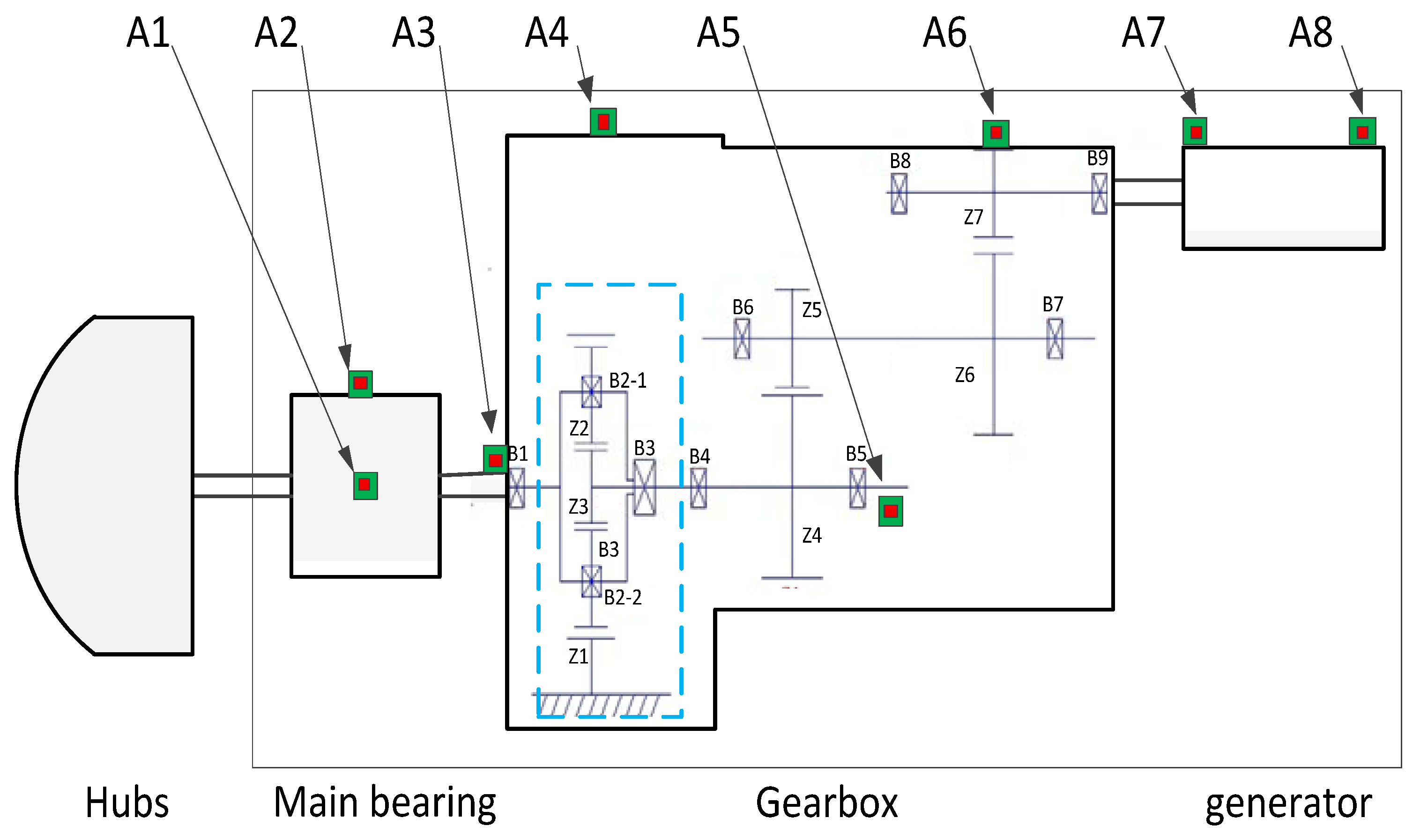
Figure 1. The block diagram of the proposed IWGP model.
Energies 11 03318 g001
Figure 2. The amplitude spectrums with different fault levels.
Energies 11 03318 g002
Figure 3. The variation of the RMS value.
Energies 11 03318 g003
Figure 4. The whitenization weight function.
Energies 11 03318 g004
Figure 5. The health indicator sequence layer and its portable value.
Energies 11 03318 g005
Figure 6. The raw and IW method processed normal WTGB vibration RMS values.
Energies 11 03318 g006
Figure 7. The vibration signals acquisition process in wind turbine generator bearing.
Energies 11 03318 g007
Figure 8. The distribution of the accelerometer on the wind turbine.
Energies 11 03318 g008
Figure 9. The comparison of the raw data and the reconstructed WPT signal in the frequency domain for different base functions: (a) dmey function, (b) db3 function, (c) haar function, (d) db2 function.
Energies 11 03318 g009
Figure 10. The WPT node energy distribution with different fault levels.
Energies 11 03318 g010
Figure 11. The comparison of the original signal and the reconstructed signal: (a) time domain; (b) frequency domain.
Energies 11 03318 g011
Figure 12. The pre-process for de-noising by EMD.
Energies 11 03318 g012
Figure 13. The IMFs decomposed by EMD.
Energies 11 03318 g013
Figure 14. The constructed signals in the frequency domain by EMD and WPT.
Energies 11 03318 g014
Figure 15. The raw and whiten health indicators: (a) RMS of training datasets; (b) EE of training datasets; (c) RMS of testing datasets; (d) EE of testing datasets.
Energies 11 03318 g015aEnergies 11 03318 g015b
Figure 16. The prediction accuracy with IWGP method.
Energies 11 03318 g016
Figure 17. The prediction accuracy with different methods: the WI health indicators.
Energies 11 03318 g017
Figure 18. The prediction accuracy with different methods: the raw health indicators.
Energies 11 03318 g018
Table 1. The detail information on the datasets.
Wind Turbine NumberData LengthSampling FrequencySensor Location
#1 (training)165 days2500 HzA8
#2 (test)169 days2500 HzA8
Table 2. The fault characteristic frequencies of the WTGB.
Fault Type Outer   Race   F O Inner   Race   F I Rolling   Element   F R
Characteristic frequency (Hz)3.133 f r 4.867 f r 2.198 f r
Variation range (Hz)57.6–87.789.6–136.340.4–61.5
Four-octave coverage (Hz)57.6–350.889.6–545.240.4–246
Table 3. Nodes energy ratio.
Waveform Number123456Mean
Nodes Energy Radio
Nodes
0–10 nodes0.69350.91890.97700.57890.67450.75070.7656
0–11 nodes0.70910.92130.97780.58960.71630.77220.7810
0–12 nodes0.73000.92510.97870.60760.74360.78700.7953
0–13 nodes0.71500.92960.97870.61730.76110.79650.7997
0–14 nodes0.79450.93380.97920.64900.79840.82190.8295

