Probabilistic Wind Power Forecasting Approach via Instance-Based Transfer Learning Embedded Gradient Boosting Decision Trees

Abstract

With the high wind penetration in the power system, accurate and reliable probabilistic wind power forecasting has become even more significant for the reliability of the power system. In this paper, an instance-based transfer learning method combined with gradient boosting decision trees (GBDT) is proposed to develop a wind power quantile regression model. Based on the spatial cross-correlation characteristic of wind power generations in different zones, the proposed model utilizes wind power generations in correlated zones as the source problems of instance-based transfer learning. By incorporating the training data of source problems into the training process, the proposed model successfully reduces the prediction error of wind power generation in the target zone. To prevent negative transfer, this paper proposes a method that properly assigns weights to data from different source problems in the training process, whereby the weights of related source problems are increased, while those of unrelated ones are reduced. Case studies are developed based on the dataset from the Global Energy Forecasting Competition 2014 (GEFCom2014). The results confirm that the proposed model successfully improves the prediction accuracy compared to GBDT-based benchmark models, especially when the target problem has a small training set while resourceful source problems are available.

1. Introduction

Wind energy has grown to an extent whereby its impact on the power system has become relevant in many regions. According to a report by the World Wind Energy Association (WWEA), the total capacity of wind turbines installed worldwide reached 539 GW at the end of 2017 [1]. In recent years, an increasing number of countries, including Germany, Ireland, Portugal, Spain, Sweden, and Uruguay, have reached a double-digit wind power share. Considering the higher variability of wind power generation, the increased wind power penetration level will introduce considerable uncertainties to power systems, resulting in higher requirements on power system transmission capacity, reserve capacity and system flexibility [2]. Probabilistic wind power forecasting is proposed to model the uncertainty of wind power by estimating the probability distribution of wind power generation. Based on the probability distribution, many decision-making applications, including unit commitment [3,4,5,6,7,8], wind power trading [9,10,11,12], reserve procurement [13,14], demand response [15,16], probabilistic power flow [17,18], and economic dispatch [19,20,21], can be developed.

To model the wind power distribution, some researchers developed a point wind power forecasting model, and subsequently, parametric models [22,23,24,25,26,27,28] and non-parametric models [29,30,31,32] were built to model the error distribution. In recent years, much attention has been paid to quantile regression. In the wind power forecasting track of the Global Energy Forecasting Competition 2014 (GEFCom2014) [32], three of the five most-effective models incorporated quantile regression to solve the wind power distribution. By utilizing the pinball loss function, quantile regression estimates the wind power quantiles directly, which has been shown to be an effective probabilistic wind power forecasting method. For example, a quantile regression forest model and a stacked random forest-gradient boosting decision trees (GBDT) model were built in [33]. These two models form a voted ensemble for forecasting the probability distribution of wind power. In [34], a quantile linear regression model was built, whereby the non-linear feature transformations of the input variable are taken as the model input. The winner of the GEFCom2014 wind power track developed a gradient boosted machine (GBM) approach for multiple quantile regression, therein fitting each quantile and zone independently [35]. Notably, the model developed in [35] utilizes the information on correlated wind farms in the other zones. The case study shows that when the information of the wind farms in the other zones is used as the input, a 2.5% decrease in the pinball loss can be achieved. Similarly, rather than solely using one numerical weather predictions (NWP) sample point measured at the location of the power plant, the work in [36] explored information from the NWP data of both the local zone and the nearby zones, which constitutes a spatial grid of NWP. By constructing new variables from the raw NWP data of the NWP grid, [36] significantly improved the forecast skill of state of the art forecasting systems by 16.09% and 12.85% for solar and wind power, respectively. The success of [35,36] suggested that introducing information of the wind farms in other zones is a viable technique to reduce the prediction error.

To utilize the information of wind power generations in other zones, this paper proposes a wind power quantile forecasting method based on instance-based transfer learning. Transfer learning focuses on solving a specific problem (target problem) using knowledge gained from different, but related problems (source problems) [37]. With this knowledge, transfer learning can improve the results achieved on a target problem [38]. Many successful applications can be found in visual adaptation [39] and text classification [40]. In instance-based transfer learning, the data of the related problems are used as training examples for the target problem [41,42]. For wind power quantile regression, the wind power generation of the wind farm in different zones shows spatial cross-correlation [43]. Therefore, it is reasonable to apply instance-based transfer learning techniques to reduce forecasting error on the target zone by introducing the data of related wind farms to the training set.

To review existing works that use instance-based transfer learning in forecasting, the work in [44] focused on adding data from the source problems (auxiliary training data) to the training process together with the data from the target problem (base training data). As the source problem set may mix with unrelated problems and the resulting negative knowledge transfers can degrade the prediction accuracy [45], thus [44] introduced a source problem selection technique based on the covariance coefficient of the load vectors. However, the selected auxiliary training data from different source problems are directly added to the training set and treated equally, neglecting the fact that the relatedness to the target problem is not the same for each source problem.

In this paper, an IBT-GBDT (instance-based transfer learning embedded gradient boosting decision trees) model is proposed. The gradient boosting decision trees algorithm is very effective in wind power generation probabilistic forecasting, which is chosen as the core forecasting method. Following the instance-based transfer learning technique, the base training data from the target problem and auxiliary training data from the source problems together constitute the training set, but with different weights assigned. To derive the weights, this paper analyzes two types of errors, i.e., random errors and systematic errors. Then, the formula for the weights, which considers the distribution of the errors, is given. However, the errors are unknown before the model is trained; thus, in practice, based on the theoretical analysis, the weights of the auxiliary training sets are solved by iteration, whereas the weight of the base training set is a hyperparameter chosen by cross-validation. As a result of the advantages of transfer learning, the combination successfully utilizes information about other zones. With the enlarged training set, the model is well trained using the GBDT algorithm, which results in the improvement in prediction accuracy. The IBT-GBDT model is tested on a public dataset from the wind track of GEFCom2014. This dataset consists of 10 zones. Measured by quantile forecasting score (QS), the results show that the IBT-GBDT method can increase the forecasting accuracy for the target zone, especially when this target problem has many closely-correlated problems and a small training set.

To the best of our knowledge, this is the first time that instance-based transfer learning has been used for wind power quantile regression. The contributions of this paper are three-fold:

• Instance-based transfer learning is utilized to increase the forecasting accuracy of probabilistic wind power forecasting. Different weights are assigned to different auxiliary training sets according to their relatedness to the target problem to reflect the real relatedness between source problems and the target problem. Based on the maximum likelihood method, the theoretical formula for the weights is derived.
• A unique method for solving the weights is proposed in this paper. The weight for a target zone is a hyperparameter chosen by cross-validation, and the weights for the source problems are solved by iteration.
• Several GBDT-based benchmark models are developed in this paper to illustrate the effect of the instanced-based transfer learning method. Compared to those benchmark models, the IBT-GBDT model earned the highest prediction accuracy.

The remainder of this paper is organized as follows. In Section 2, the mathematical formulation of the proposed IBT-GBDT model and the corresponding training method are described. Case studies are conducted to validate the proposed approach in Section 3. Finally, Section 4 gives a summary of this paper.

2. The Instance-Based Transfer Learning Embedded Gradient Boosting Decision Trees

At the beginning of this section, the methodology of GBDT and its application in quantile regression are introduced. Then, the architecture of the IBT-GBDT model is described. Finally, the weight formula and the corresponding iterative weight-solving algorithm are derived.

2.1. Gradient Boosting Decision Trees for Quantile Regression

2.1.1. Pinball Loss Function and Weighted Pinball Loss

The pinball loss function is an error measure for quantile regression. Given a target percentile $\tau$, $f_{\tau }(·)$ denotes the predictive function for the wind power quantile. The corresponding pinball loss, denoted by $l_{\tau }(y,f_{\tau }\left(\mathbf{X}\right))$, is defined as:

$$l_{\tau }(y,f_{\tau }\left(\mathbf{X}\right))=\left\{\begin{array}{c}\tau (y-f_{\tau }\left(\mathbf{X}\right)),\mathbf{y}>{\mathbf{f}}_{ø}\left(\mathbf{X}\right)\hfill \\ (\mathbf{1}-\tau )(f_{\tau }\left(\mathbf{X}\right)-\mathbf{y}),\mathbf{y}\le {\mathbf{f}}_{ø}\left(\mathbf{X}\right).\hfill \end{array}\right.$$

(1)

where $\mathbf{X}$ denotes the model inputs such as the weather, wind speed, and wind direction. y denotes the actual wind power generation.

For a sample set denoted by $\mathbf{S}$, by summing the pinball losses across all samples from $\mathbf{S}$, the pinball loss of the set $\mathbf{S}$ is obtained. As some data points contribute more than others, large weights are assigned to the samples with higher contributions. In this case, the weighted pinball loss for the sample set $\mathbf{S}$ is defined as the weighted sum of all the pinball losses of samples from $\mathbf{S}$. Let $({\mathbf{X}}_i,y_i)$ denote the ith sample of $\mathbf{S}$ and $w_i$ denote the corresponding weight (the determination of $w_i$ depends on $({\mathbf{X}}_i,y_i)$, which is introduced in detail in Section 2.3). The weighted pinball loss is defined as:

$$\begin{array}{cc}\hfill L_{\tau }(y,f_{\tau }\left(\mathbf{X}\right))& =\sum _{i=1}^N{w}_i{l}_{\tau }(y_i,f_{\tau }\left({\mathbf{X}}_i\right))\hfill \\ & =\tau \sum _{y_i>f_{\tau }\left({\mathbf{X}}_i\right)}{w}_i(y_i-f_{\tau }\left({\mathbf{X}}_i\right))\hfill \\ & +(1-\tau )\sum _{y_i\le f_{\tau }\left({\mathbf{X}}_i\right)}{w}_i(f_{\tau }\left({\mathbf{X}}_i\right)-y_i).\hfill \end{array}$$

(2)

2.1.2. Gradient Boosting Decision Trees with Weighted Pinball Loss

Gradient boosting is a machine learning technique for regression and classification problems, which produces a prediction model in the form of an ensemble of base learners. Typically, gradient boosting is used with decision trees of a fixed size as base learners, e.g., Classification And Regression Trees (CART). By utilizing the weighted pinball loss, the use of gradient boosting decision trees (GBDT) becomes an effective technique for quantile regression.

GBDT builds the model in a stage-wise manner. In every stage, the target is to fit the residual error. $f^{\left(t\right)}$ denotes the fitted function after stage t. The number of boosting stages is denoted by T. Before the tth stage, the residual error for point i is:

$${\epsilon }_i^{(t-1)}=y_i-f^{(t-1)}\left({\mathbf{X}}_i\right).$$

(3)

$v_i^{\left(t\right)}$ denotes the fitted value on the ith sample in stage t.

$$f^{\left(t\right)}\left({\mathbf{X}}_{\mathbf{i}}\right)=f^{(t-1)}\left({\mathbf{X}}_{\mathbf{i}}\right)+v_i^{\left(t\right)}$$

(4)

After the residual error is fitted, the updated weighted pinball loss for the sample set $\mathbf{S}$ becomes:

$$\begin{array}{cc}\hfill L_{\tau }^{\left(t\right)}& =\tau \sum _{v_i^{\left(t\right)}<{\epsilon }_i^{(t-1)}}{w}_i({\epsilon }_i^{(t-1)}-v_i^{\left(t\right)})\hfill \\ & +(1-\tau )\sum _{v_i^{\left(t\right)}\ge {\epsilon }_i^{(t-1)}}{w}_i(v_i^{\left(t\right)}-{\epsilon }_i^{(t-1)}).\hfill \end{array}$$

(5)

The gradient of $L_{\tau }^{\left(t\right)}$ on $v_i^{\left(t\right)}$ is:

$$g_i^{\left(t\right)}=\frac{\partial L_{\tau }^{\left(t\right)}}{\partial v_i^{\left(t\right)}}=\left\{\begin{array}{c}-w_i\tau ,v_i^{\left(t\right)}<{\epsilon }_i^{(t-1)}\hfill \\ w_i(1-\tau ),v_i^{\left(t\right)}\ge {\epsilon }_i^{(t-1)}.\hfill \end{array}\right.$$

(6)

Recall the definition of gradient boosting. The base learner should fit the negative gradient of the loss function ($-g_i^{\left(t\right)}$). When choosing CART as the base learner, the updated weighted pinball loss is:

$$\begin{array}{cc}\hfill L_{\tau }^{\left(t\right)}& =\tau \sum _{k=1}^{K^{\left(t\right)}}\sum _{{\rho }_k^{\left(t\right)}<{\epsilon }_i^{(t-1)}}{w}_i({\epsilon }_i^{(t-1)}-{\rho }_k^{\left(t\right)})\hfill \\ & +(1-\tau )\sum _{k=1}^{K^{\left(t\right)}}\sum _{{\rho }_k^{\left(t\right)}\ge {\epsilon }_i^{(t-1)}}{w}_i({\rho }_k^{\left(t\right)}-{\epsilon }_i^{(t-1)}),\hfill \end{array}$$

(7)

where ${\rho }_k^{\left(t\right)}$ denotes the value of the kth tree leaf in stage t and $K^{\left(t\right)}$ denotes the number of tree leaves in stage t. To minimize the weighted pinball loss function $L_{\tau }^{\left(t\right)}$, we take the partial derivative of $L_{\tau }^{\left(t\right)}$ with respect to the value of the kth node (${\rho }_k^{\left(t\right)}$).

$$\begin{array}{cc}\hfill \frac{\partial L_{\tau }^{\left(t\right)}}{\partial {\rho }_k^{\left(t\right)}}& =-\tau \sum _{{\rho }_k^{\left(t\right)}<{\epsilon }_i^{(t-1)}}{w}_i+(1-\tau )\sum _{{\rho }_k^{\left(t\right)}\ge {\epsilon }_i^{(t-1)}}{w}_i\hfill \end{array}$$

(8)

${\rho }_k^{\left(t\right)}$ is chosen according to the following equation.

$${\rho }_k^{\left(t\right)}=arg\underset{{\rho }_k^{\left(t\right)}}{min}\left|\tau \sum _{{\rho }_k^{\left(t\right)}<{\epsilon }_i^{\left(t\right)}}{w}_i-(1-\tau )\sum _{{\rho }_k^{\left(t\right)}\ge {\epsilon }_i^{\left(t\right)}}{w}_i\right|$$

(9)

2.1.3. Hyperparameters of Gradient Boosting Decision Trees

In the application of the GBDT algorithm, hyperparameter tuning is crucially important. In this paper, we consider several key hyperparameters, which can be classified into two groups: (1) regression tree-related hyperparameters; (2) gradient boosting-related hyperparameters.

The regression tree-related hyperparameters are (1) maximum depth $D_{max}$ and (2) minimum number of samples in leaf node $N_{leaf}$. Maximum depth controls the number of nodes used in the individual tree. The common value of maximum depth is between five and nine, which gives a suitable model complexity for the decision tree as a base learner of gradient boosting. The minimum number of samples in the leaf node is always between 20 and 80 [36].

The gradient boosting-related hyperparameters are (1) the number of boosting iterations T, (2) learning rate $\lambda$, and (3) bag fractions $bag$. The bag fraction stands for the fraction of samples to be used to train the individual decision tree and is a real number satisfying $bag\in [0,1]$. The number of boosting stages controls the number of trees used in the model. With sufficient boosting stages, it is a common pattern that the smaller the learning rate is, the better the generalization achieved [46]. However, the quantile GBDT model has to repeat the training process 99 times at each percentile ($\tau =0.01,0.02,\cdots ,0.99$), which is time consuming. Considering the computation time, the value of $\lambda$ is chosen as 0.05. For this specific $\lambda$, the optimal value of T is between 400 and 800 [36].

The optimal values for these super parameters are determined by cross-validation, which will be discussed later.

2.2. The Architecture of IBT-GBDT

Consider M source problems $\left\{P^{\left(m\right)}\right\}$, where m is the source problem index. When training the forecasting model for the target zone, the sample data of the target problem (base training data) constitute the training set. In an ideal scenario, wind power generations of the wind farm in different zones are strongly correlated. For the wind power quantile regression in the target zone, other than the base training data, the auxiliary training data can be added directly to the training set. With the enlarged training set, the model can be better trained, and the forecasting error will thus be reduced. In this case, the samples from the auxiliary training set and base training set satisfy the following equations.

$$\begin{array}{c}{y}_i^{\left(m\right)}=f({\mathbf{X}}_i^{\left(m\right)})+{\epsilon }_i^{\left(m\right)}\hfill \\ y_i^{\left(\mathrm{target}\right)}=f({\mathbf{X}}_i^{\left(\mathrm{target}\right)})+{\epsilon }_i^{\left(\mathrm{target}\right)},\hfill \end{array}$$

(10)

where f denotes the real mapping function between the input variable ${\mathbf{X}}_i^{\left(\mathrm{target}\right)}$ and the wind power $y_i^{\left(\mathrm{target}\right)}$ for the target problem; ${\mathbf{X}}_i^{\left(m\right)}$ and $y_i^{\left(m\right)}$ represent the ith input variable and output wind power from the mth source problem, respectively; and ${\epsilon }_i^{\left(\mathrm{target}\right)}$ and ${\epsilon }_i^{\left(m\right)}$ denote the random error for samples from $P^{\left(\mathrm{target}\right)}$ and $P^{\left(m\right)}$, respectively.

However, in practice, the cross-correlation between the target problem and source forecasting problems is not ideal. In the worst case, the source problem set may be mixed with totally irrelevant problems. Therefore, the systematic error ${\delta }_i^{\left(m\right)}$ is introduced to denote the imperfect relatedness of $P^{\left(m\right)}$ to $P^{\left(\mathrm{target}\right)}$. With the systematic error considered, Formula (10) becomes:

$$\begin{array}{c}{y}_i^{\left(m\right)}=f^{\left(m\right)}({\mathbf{X}}_i^{\left(m\right)})+{\delta }_i^{\left(m\right)}+{\epsilon }_i^{\left(m\right)}\hfill \\ y_i^{\left(\mathrm{target}\right)}=f({\mathbf{X}}_i^{\left(\mathrm{target}\right)})+{\epsilon }_i^{\left(\mathrm{target}\right)}.\hfill \end{array}$$

(11)

where $f^{\left(m\right)}$ denotes the real mapping function between the input variable ${\mathbf{X}}_i^{\left(m\right)}$ and the wind power $y_i^{\left(m\right)}$ for the mth source problem. $f^{\left(m\right)}$ is different from f.

In this case, the base training data and auxiliary training data should not be treated equally. In this paper, different weights are assigned to the target problem and source problems. The weight of the base training set is defined as $w^{\left(\mathrm{target}\right)}$, and $w^{\left(m\right)}$ denotes the weight of the mth auxiliary training set. $w^{\left(m\right)}$ should reflect the relatedness of different source problems $P^{\left(m\right)}$ to the target problem. A larger $w^{\left(m\right)}$ for $P^{\left(m\right)}$ implies a stronger relatedness to the target problem. The formula for weights is derived in Section 2.3. In this formula, the weights are calculated based on the performance of the GBDT model. Based on the formula for weights, an iterative algorithm is developed to solve the weight, where the weights are adjusted according to the weight formula in every iteration. Then, the updated weight is sent back to the GBDT model. The iteration stops when the weights converge.

When the target percentile $\tau$ changes, this paper assumes that the relatedness between the target problem and source problems does not change. Thus, the weights are the same for different quantiles and only need to be solved once. Therefore, the IBT-GBDT described in this paper is divided into two training steps. In Step 1, the weight is solved, and the quantile regression model with $\tau =0.5$ is trained. In Step 2, the weight from Step 1 is assigned to different datasets accordingly, and then, the quantile regression with $\tau =0.01\sim 0.49$ and $0.51\sim 0.99$ is solved. In both two steps, the inner GBDT model is trained using the algorithm described in Section 2.1.2. The structure of the proposed IBT-GBDT model is depicted in Figure 1.

2.3. Derivation of the Weight Formula

The analysis in [27] shows that the error distribution of wind power generation forecasting is a heavy-tailed distribution. Thus, when solving the quantile regression model with $\tau =0.5$ in Step 1, we assume that the random variants ${\delta }^{\left(m\right)}+{\epsilon }^{\left(m\right)}$ and ${\epsilon }_i^{\left(\mathrm{target}\right)}$ are independent and follow the Laplace distribution. The expressions are:

$$\begin{array}{c}{\epsilon }^{\left(\mathrm{target}\right)}\sim \mathrm{Laplace}(0,b_{\epsilon }^{\left(\mathrm{target}\right)})\hfill \\ {\delta }^{\left(m\right)}+{\epsilon }^{\left(m\right)}\sim \mathrm{Laplace}(0,b_{\delta +\epsilon }^{\left(m\right)}).\hfill \end{array}$$

(12)

where $b_{\epsilon }^{\left(\mathrm{target}\right)}$ and $b_{\delta +\epsilon }^{\left(m\right)}$ represent the scale parameter of ${\epsilon }^{\left(\mathrm{target}\right)}$ and ${\delta }^{\left(m\right)}+{\epsilon }^{\left(m\right)}$, respectively.

For the hypothesis set of the prediction functions $f_{\theta }$ ($\theta$ is a parameter), the likelihood of the prediction function $f_{\theta }$ being the correct prediction function is:

$$\begin{array}{cc}\hfill Likelihood\left(\theta \right)& =\log \left(P\right(Y|X;\theta ))\hfill \\ & =N^{\left(\mathrm{target}\right)}log\frac{1}{2b_{\epsilon }^{\left(\mathrm{target}\right)}}-\sum _{i=1}^{N^{\left(\mathrm{target}\right)}}\frac{1}{b_{\epsilon }^{\left(\mathrm{target}\right)}}\left|y_i^{\left(\mathrm{target}\right)}-f_{\theta }({\mathbf{X}}_i^{\left(\mathrm{target}\right)})\right|\hfill \\ & +\sum _{m=1}^M{N}^{\left(m\right)}log\frac{1}{2b_{\delta +\epsilon }^{\left(m\right)}}-\sum _{m=1}^M\sum _{i=1}^{N^{\left(m\right)}}\frac{1}{b_{\delta +\epsilon }^{\left(m\right)}}\left|y_i^{\left(m\right)}-f_{\theta }({\mathbf{X}}_i^{\left(m\right)})\right|.\hfill \end{array}$$

(13)

Using the maximum likelihood method, the most likely value for the parameter $\widehat{\theta }$ is:

$$\begin{array}{c}\widehat{\theta }=argmax\left(Likelihood\left(\theta \right)\right)\hfill \\ =argmin\left({\displaystyle \sum _{m=1}^M}{\displaystyle \sum _{i=1}^{N^{\left(m\right)}}}\frac{1}{b_{\delta +\epsilon }^{\left(m\right)}}\left|y_i^{\left(m\right)}-f_{\theta }({\mathbf{X}}_i^{\left(m\right)})\right|\right.\hfill \\ +\left.{\displaystyle \sum _{i=1}^{N^{\left(\mathrm{target}\right)}}}\frac{1}{b_{\epsilon }^{\left(\mathrm{target}\right)}}\left|y_i^{\left(\mathrm{target}\right)}-f_{\theta }({\mathbf{X}}_i^{\left(\mathrm{target}\right)})\right|\right).\hfill \end{array}$$

(14)

The target optimization function for solving the most likely prediction function $f_{\widehat{\theta }}$ is:

$$loss=\sum _{m=1}^M\frac{1}{b_{\delta +\epsilon }^{\left(m\right)}}\sum _{i=1}^{N^{\left(m\right)}}\left|y_i^{\left(m\right)}-f_{\widehat{\theta }}({\mathbf{X}}_i^{\left(m\right)})\right|+\frac{1}{b_{\epsilon }^{\left(\mathrm{target}\right)}}\sum _{i=1}^{N^{\left(\mathrm{target}\right)}}\left|y_i^{\left(\mathrm{target}\right)}-f_{\widehat{\theta }}({\mathbf{X}}_i^{\left(\mathrm{target}\right)})\right|.$$

(15)

According to (15), the weight formulas for $w^{\left(\mathrm{target}\right)}$ and $w^{\left(m\right)}$ are:

$$w^{\left(\mathrm{target}\right)}=1/b_{\epsilon }^{\left(\mathrm{target}\right)}$$

(16)

$$w^{\left(m\right)}=1/b_{\delta +\epsilon }^{\left(m\right)}.$$

(17)

For weights, only their relative size matters. Thus, this paper normalizes the weights of the source problems $w^{\left(m\right)}$ to the range 0–1.

$$w^{\left(m\right)}=\underset{m}{min}(b_{\delta +\epsilon }^{\left(m\right)})/b_{\delta +\epsilon }^{\left(m\right)}$$

(18)

The corresponding $w^{\left(\mathrm{target}\right)}$ becomes:

$$w^{\left(\mathrm{target}\right)}=\underset{m}{min}(b_{\delta +\epsilon }^{\left(m\right)})/b_{\epsilon }^{\left(\mathrm{target}\right)}.$$

(19)

2.4. Iterative Weight Assignment Algorithm

According to (18) and (19), the calculation of weights depends on the error distributions, and the error is calculated after the model is trained; however, the model is trained after the weights are set. To solve for the circular dependency, an iterative algorithm is presented in this paper, where $w^{\left(m\right)}$ is solved via iteration, while $w^{\left(\mathrm{target}\right)}$ is a hyperparameter chosen in advance via cross-validation.

Because the relatedness between all the source problems $P^{\left(m\right)}$ and the target problem $P^{\left(\mathrm{target}\right)}$ is initially unknown, all the source problems $P^{\left(m\right)}$ are assigned to the same weight (according to (18), the initial value for all $w^{\left(m\right)}$ is one). With $w^{\left(\mathrm{target}\right)}$ and $w^{\left(m\right)}$ determined, the inner quantile regression model is trained using the gradient boosting decision trees described in Section 2.1.2. After the inner layer is trained, $b_{\delta +\epsilon }^{\left(m\right)}$ (the scale parameter of the Laplace error distribution) is calculated. The weights $w^{\left(m\right)}$, based on (18), are updated according to the corresponding $b_{\delta +\epsilon }^{\left(m\right)}$. With the updated $w^{\left(m\right)}$, the next iteration begins. Finally, the outer iteration stops when every $w^{\left(m\right)}$ converges (Equation (18) holds simultaneously). The pseudocode of the weight assignment algorithm is described in Algorithm 1.

Algorithm 1 Weight assignment via iteration and validation (pseudocode).

1: Choose $w^{\left(\mathrm{target}\right)}$ 2: Initialize every $w^{\left(m\right)}$ to 1 3: repeat 4:   Complete the training of the inner quantile GBDT layer with $\tau =0.5$ according to the updated weight $w^{\left(m\right)}$ 5:   Calculate $b_{\delta +\epsilon }^{\left(m\right)}$ 6:   Calculate $w^{\left(m\right)}$ according to (18) 7: until Every $w^{\left(m\right)}$ converges 8: Complete the training of the inner quantile GBDT layer with $\tau =0.01\sim 0.49$ and $0.51\sim 0.99$ based on the converged weight $w^{\left(m\right)}$

3. Application and Results

3.1. Data Specification

To examine the IBT-GBDT model proposed in this paper, the model is tested on a public dataset from the probabilistic wind power forecasting track of GEFCom2014 (the dataset of GEFCom2014 is available in the Supplementary Material of [32]). The aim of this track was to forecast the normalized wind power generation in 10 zones, corresponding to 10 wind farms in Australia. The competition consisted of 15 tasks. The first three tasks were trial tasks, and the last 12 tasks were the evaluation tasks. To mimic real-world forecasting processes, the tasks were designed in a rolling forecasting manner. In the first trail task, months of data were provided as training data. With one month of incremental data released, the aim of each task was to forecast the wind power generation of the next month. The provided input included a 10-m wind speed vector and a 100-m wind speed vector. The desired output was the probabilistic distribution of wind power generation described by multiple quantiles. For each task, the quantile regression model was trained independently. The data period of the corresponding task is listed in

Table 1. Data period of the scoring task.

Task	Training Set	Testing Set
Task 1	January 2012–December 2012	January 2013
Task 2	January 2012–January 2013	February 2013
Task 3	January 2012–February 2013	March 2013
Task 4	January 2012–March 2013	April 2013
Task 5	January 2012–April 2013	May 2013
Task 6	January 2012–May 2013	June 2013
Task 7	January 2012–June 2013	July 2013
Task 8	January 2012–July 2013	August 2013
Task 9	January 2012–August 2013	September 2013
Task 10	January 2012–September 2013	October 2013
Task 11	January 2012–October 2013	November 2013
Task 12	January 2012–November 2013	December 2013

.

3.2. Benchmark Models

In GEFCom2014, GBDT was shown to be a very effective algorithm for probabilistic forecasting of wind power, as GBDT was used in the top two effective models. In this paper, three GBDT-based models were developed and chosen as the benchmark models. The first one is the DL-GBDT [35], which was the winner of the wind power forecasting track of GEFCom2014. The authors of this paper reproduced the DL-GBDT model with exactly the same structure, input features, and hyperparameters. The last two benchmark models were the basic GBDT models that were developed to exhibit the effectiveness of the weight assignment algorithm. One was the GBDT model trained only by the base training data. The other was the GBDT model trained by both the base training data and auxiliary training data.

3.3. Feature Selection

The input data provided were hourly wind forecasts of the zonal and meridional wind components at 10 and 100 m, for ten separate (but correlated) wind zones. Based on the model input, the wind speed (WS), wind direction (WD), and wind energy (WE) are defined as follows, where u and v are the wind components provided.

$$\begin{array}{c}\mathrm{WS}=\sqrt{u^2+v^2}\hfill \\ \mathrm{WD}=180/\pi \times arctan(u,v)\hfill \\ \mathrm{WE}=0.5\times w{s}^3\hfill \end{array}$$

(20)

In DL-GBDT, features are derived from the provided model input by feature engineering, and different combinations of input features are tested by cross-validation. As a result, the input features of DL-GBDT model are very effective for the quantile model fit. Therefore, the proposed IBT-GBDT model chose the same input features as the DL-GBDT model, except the feature “hour” was added. The corresponding input features for the forecasting model of different zones are listed in

Table 2. Input features for forecasting model of each zone.

Feature	Zones
Current 10-m energy	All zones
Current energy	All zones
Current 10-m direction	All zones
Current direction	All zones
Hour of day	All zones
−1 period energy	All zones, but Zone 1
−2 period energy	All zones, but Zone 1
−3 period energy	Zones 2, 3, 5, 6, 7
+1 period energy	All zones
+3 period energy	Zones 2, 3, 5, 6, 7
+4 period energy	Zone 1
−1 period direction	Zones 1, 6
+1 period direction	Zones 1, 6
Average energy, Periods −3–0	All zones, but Zones 1, 2, 7
Average energy, Periods 0–+3	All zones
Standard deviation of direction, Periods −3–0	Zones 1, 2, 3, 10
Direction difference: 100 m and 10 m	All zones
Energy ratio: 100 m and 10 m	All zones
Percentage speed change: current and −1 period	All zones

Note: all values are for the 100-m wind speed, unless otherwise specified.

.

3.4. Error Measure

The sharpness and reliability are two key measures for probabilistic forecasting. According to [32], the wind power quantile forecasting score (QS) is defined. QS is a comprehensive evaluation of sharpness and reliability, which is the average of pinball loss over all target percentiles. For the convenience of comparison, the target percentiles were chosen to be $\tau =0.01,0.02,\cdots 0.99$, the same as in GEFCom2014.

$$\mathrm{QS}=\frac{1}{99}\left(\sum _{\tau =0.01}^{0.99}{L}_{\tau }(y,f\left(x\right))\right)$$

(21)

3.5. Hyperparameter Tuning through Cross-Validation

For IBT-GBDT and the two basic GBDT models, the hyperparameters were determined through cross-validation. The hyperparameters included decision tree-related hyperparameters and gradient boosting-related hyperparameters. For IBT-GBDT, there was another hyperparameter $w^{\mathrm{target}}$. The data of the first three trial tasks were divided into five distinct parts, which constituted the five-fold cross-validation sets. A brief grid search was conducted to determine the optimal value of those hyperparameters. The result suggested that two sets of parameters should be used, one for percentiles in the middle range 0.16–0.84 and the for other percentiles.

Table 3. Hyperparameter settings.

	$\mathit{\tau }=0.16\sim 0.84$				$\mathit{\tau }=0.01\sim 0.15$ and $0.85\sim 0.99$
Model	GBDT1	GBDT2	DL-GBDT	IBT-GBDT	GBDT1	GBDT2	DL-GBDT	IBT-GBDT
$D_{max}$	7	7	7	8	5	5	5	6
$N_{leaf}$	30	30	30	30	30	30	30	30
T	500	500	500	500	400	400	400	500
$\lambda$	0.05	0.05	0.05	0.05	0.05	0.05	0.05	0.05
$bag$	0.75	0.75	0.75	0.75	0.75	0.75	0.75	0.75

presents the hyperparameter settings for the proposed IBT-GBDT model and the GBDT-based benchmark models (note: in the following tables, GBDT¹ represents the GBDT model trained by the base training data and GBDT² the GBDT model trained by both the base training data and the auxiliary training data.)

Table 4. $w^{\mathrm{target}}$ settings for the IBT-GBDT model.

Zone Index	1	2	3	4	5	6	7	8	9	10
$w^{\mathrm{target}}$	50	20	100	100	20	50	50	20	20	100

presents the optimal value of $w^{\mathrm{target}}$ in the proposed IBT-GBDT model of different zones.

3.6. Illustration of Training Process

To illustrate the training process of the IBT-GBDT model, wind power generation quantile forecasting for Zone 7 in the fourth evaluation task was chosen as the target problem. The auxiliary training sets were the data of wind power generation in zones other than Zone 7.

The cross-validation results showed that the best value of the hyperparameter $w^{\mathrm{target}}$ was 50. Thus, 50 was chosen as the weight of the dataset from Zone 7 (target zone). The weights of the others zones were initialized to one. Then, the quantile regression model with $\tau =0.5$ was trained according to Step 1 of Algorithm 1. The converging process of the weights is presented in

Table 5. Weights of the training sets from different zones after each iteration.

Zone	Iteration Step
	Initial	1	2	3	4	5	6	7	8
Zone 1	1	0.546	0.538	0.539	0.535	0.535	0.536	0.535	0.535
Zone 2	1	0.835	0.819	0.816	0.811	0.817	0.816	0.817	0.817
Zone 3	1	0.380	0.364	0.363	0.361	0.364	0.363	0.363	0.363
Zone 4	1	0.464	0.447	0.449	0.445	0.446	0.448	0.448	0.448
Zone 5	1	0.331	0.314	0.315	0.312	0.315	0.316	0.315	0.315
Zone 6	1	0.294	0.281	0.281	0.278	0.282	0.282	0.282	0.282
Zone 7	50	50	50	50	50	50	50	50	50
Zone 8	1	1	1	1	1	1	1	1	1
Zone 9	1	0.681	0.670	0.671	0.667	0.671	0.670	0.671	0.671
Zone 10	1	0.208	0.201	0.201	0.199	0.201	0.201	0.201	0.201

.

Table 5 shows that the weights converged after almost seven iterations. According to Table 5, the weight of Zone 8 always had the value of one. This means Zone 8 had the highest relatedness to Zone 7 (the same result was also given in [33]).

For the trained quantile regression model with $\tau =0.5$, the pinball losses on the base training set and auxiliary training sets are calculated and shown in

Table 6. Pinball loss after each iteration step.

Zone	Iteration Step
	1	2	3	4	5	6	7
Zone 1	0.0682	0.0686	0.0686	0.0686	0.0687	0.0686	0.0686
Zone 2	0.0542	0.0546	0.0547	0.0547	0.0547	0.0549	0.0548
Zone 3	0.0796	0.0812	0.0813	0.0813	0.0813	0.0812	0.0814
Zone 4	0.0734	0.0746	0.0745	0.0747	0.0748	0.0745	0.0747
Zone 5	0.0850	0.0871	0.0870	0.0872	0.0870	0.0867	0.0871
Zone 6	0.0883	0.0902	0.0903	0.0904	0.0903	0.0899	0.0903
Zone 7	0.0394	0.0391	0.0390	0.0389	0.0390	0.0389	0.0390
Zone 8	0.0509	0.0508	0.0508	0.0507	0.0509	0.0508	0.0509
Zone 9	0.0513	0.0516	0.0516	0.0517	0.0517	0.0516	0.0517
Zone 10	0.1015	0.1030	0.1033	0.1033	0.1033	0.1031	0.1033

. Compared to the training loss after the first iteration, the training loss for zones except Zone 7 and Zone 8 increased after the second iteration. The reason is that the weights of these training sets dropped after the first iteration; thus, the inner GBDT algorithm was less fit to these training sets in the second iteration.

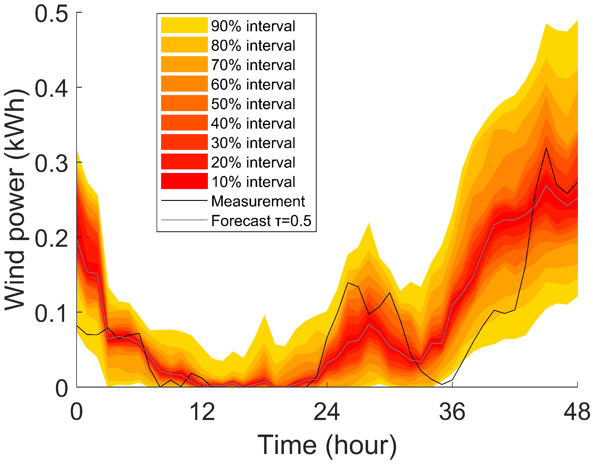
After the weight is determined, Step 2 of Algorithm 1 is executed. The wind power quantiles were forecast for the test set of Zone 7. Line plots of different prediction intervals, measurements, and forecast medium during the first 48 h are drawn in Figure 2.

3.7. The Relationship between Forecasting Error and $w^{\left(\mathrm{target}\right)}$

As stated above, $w^{\left(\mathrm{target}\right)}$ is a hyperparameter. To illustrate the effect of $w^{\left(\mathrm{target}\right)}$, for Zone 7, the relationship between QS and the hyperparameter $w^{\left(\mathrm{target}\right)}$ is drawn in Figure 3.

As $w^{\left(\mathrm{target}\right)}$ increases from 2–500, Figure 3 shows that the QS is first decreasing, but then increases. The reason is as follows. If $w^{\left(\mathrm{target}\right)}$ is too small, the model is more like a common model of all the zones, where negative transfer occurs. When $w^{\left(\mathrm{target}\right)}$ is too large, the model is more like a model trained only on data of the target zone, and no positive transfer is involved. When $w^{\left(\mathrm{target}\right)}$ is given a suitable value, the positive transfer is strengthened, whereas the negative transfer is prevented; thus, the QS obtained the best result.

3.8. Analysis on Model Reliability

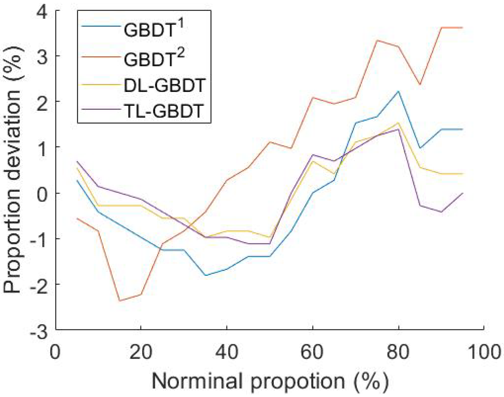
For any probabilistic forecasting method, reliability is seen as a primary requirement [47]. For the TL-GBDT model and benchmark models, the average proportion deviations between nominal and empirical proportions [47], which is the measure of reliability, are depicted in Figure 4.

According to Figure 4, the effectiveness of these models is analyzed. For all these GBDT-based methods, the quantiles were slightly overestimated for proportions lower than 0.5 and slightly underestimated for proportions above that value, which indicates that the corresponding predictive distributions were slightly too narrow. Among them, the worst-performing model was the GBDT model trained with both base training data and auxiliary training data. Negative transfer should be the main reason causing this. The second worst-performing model was the GBDT model trained with base training data. Comparing with the IBT-GBDT model, those two basic GBDT models did not perform well when the target percentile $\tau$ was between 80 and 95. For those quantiles, the distribution of training data was sparser, and the complicated model would easily overfit the training data; whereas for IBT-GBDT, with more training data, the over-fitting was suppressed.

To further evaluate the reliability of probabilistic forecasting, average coverage error (ACE) is introduced, which is defined as:

$$\begin{array}{c}{\mathrm{ACE}}_{\tau }=\frac{1}{n}{\displaystyle \sum _{i=1}^n}{C}_i\times 100\%-(1-\tau )\times 100\%,\hfill \end{array}$$

(22)

where $C_i$ is the indicative function of whether $y_i$ are covered by the prediction interval.

For any probabilistic forecasting model, the reliability may not be the same in different forecast horizons. Thus, the proposed model and benchmark models were tested on different forecast horizons. Measured by the ACE (the chosen prediction interval nominal confidences (PINCs) is 90%), a comparison of the reliability across different forecast horizons is shown in

Table 7. Comparison of the criterion average coverage error (ACE) (%).

Model	GBDT1	GBDT2	DL-GBDT	IBT-GBDT
First Week	−2.59	−3.10	−1.87	−2.21
Second Week	−2.64	−4.60	−2.77	−2.84
Third Week	1.03	1.51	0.92	0.63
Fourth Week	0.47	0.82	0.38	0.27

.

According to the results, the criteria ACE maintained within certain ranges in all forecasting horizons, which indicates that the proposed IBT-GBDT model achieved a rather high reliability in short probabilistic forecasting.

3.9. Comparison of Forecasting Error

In this paper, the forecasting errors were measured by the quantile score (QS), which was defined in (21). By definition, the QS of a model is the average of the pinball loss over all target percentiles. However, for different probabilistic wind power forecasting methods, their performance on different target percentiles is uneven. Thus, their pinball losses on several selected percentiles are listed and compared in

Table 8. The pinball loss of the IBT-GBDT model and benchmark models.

$\mathit{\tau }$	GBDT1	GBDT2	DL-GBDT	IBT-GBDT	Improvement on GBDT1	Improvement on GBDT2	Improvement on DL-GBDT
0.1	0.0150	0.0216	0.0139	0.0132	12.25%	38.84%	4.94%
0.2	0.0250	0.0329	0.0237	0.0230	7.83%	29.92%	3.05%
0.3	0.0323	0.0367	0.0315	0.0310	4.10%	15.59%	1.56%
0.4	0.0367	0.0403	0.0362	0.0359	2.18%	10.87%	0.83%
0.5	0.0396	0.0424	0.0392	0.0390	1.35%	7.98%	0.42%
0.6	0.0379	0.0422	0.0375	0.0372	1.68%	11.73%	0.71%
0.7	0.0360	0.0407	0.0352	0.0347	3.67%	14.65%	1.44%
0.8	0.0291	0.0377	0.0278	0.0270	7.33%	28.40%	2.89%
0.9	0.0186	0.0258	0.0174	0.0166	10.63%	35.63%	4.18%

.

When the target percentile $\tau$ is away from the central percentile, Table 8 shows that the improvement of the IBT-GBDT model over the DL-GBDT model is larger. The reason is discussed in the following. Around the edge of the distribution of the wind power generation, the training data were relatively scarce and had higher volatility. Furthermore, according to the definition of pinball loss, these higher volatility data had higher weights when the target percentile $\tau$ was away from the central percentile. Those training samples with high volatility caused the quantile regression model to fluctuate more, which led to lower predictive accuracy. In the proposed IBT-GBDT model, the volatility and variation of training data were reduced when more training data were available; whereas for the DL-GBDT model, the shortage of training data and the resulting high volatility still existed. This explains why the proposed IBT-GBDT model was more effective when the target percentile $\tau$ was away from the central percentile.

In addition, according to the bias variance theory, a complicated model will easily overfit a small dataset, but a complicated model is better than a simple model when more data are available. For the tree-based model, max depth $D_{max}$ reflects the complexity of the model. In Table 3, the validation result shows that the optimal value of $D_{max}$ in the IBT-GBDT model is larger than the optimal value of $D_{max}$ of the other benchmark models. This means, with more training data available in IBT-GBDT, the training dataset was large enough for the IBT-GBDT model with higher model complexity getting the upper hand, which led to the improvement in prediction accuracy.

To further test the applicability of the proposed IBT-GBDT model, this model was then applied to the zones other than Zone 7. For different zones, the QS of IBT-GBDT model was calculated and compared with the QS of the benchmark models in

Table 9. The QS improvement of the IBT-GBDT model over the benchmark models.

Zone	GBDT1	GBDT2	DL-GBDT	IBT-GBDT	Improvement on GBDT1	Improvement on GBDT2	Improvement on DL-GBDT
Zone 1	0.0257	0.0389	0.0251	0.0248	3.62%	36.22%	1.39%
Zone 2	0.0236	0.0294	0.0229	0.0226	4.27%	23.07%	1.05%
Zone 3	0.0302	0.0386	0.0294	0.0293	3.02%	24.25%	0.54%
Zone 4	0.0342	0.0439	0.0332	0.0327	4.24%	25.39%	1.50%
Zone 5	0.0338	0.0409	0.0330	0.0327	3.40%	20.15%	0.94%
Zone 6	0.0356	0.0443	0.0349	0.0346	2.89%	21.90%	0.86%
Zone 7	0.0271	0.0324	0.0262	0.0256	5.57%	21.05%	2.22%
Zone 8	0.0299	0.0329	0.0288	0.0281	5.90%	14.65%	2.40%
Zone 9	0.0311	0.0342	0.0303	0.0297	4.55%	13.09%	1.94%
Zone 10	0.0435	0.0538	0.0428	0.0421	3.22%	21.76%	1.75%

.

According to Table 9, the QS improvement over DL-GBDT achieved by IBT-GBDT ranged from 0.54%–2.40% for different zones, and the average improvement was 1.46%. Furthermore, for different tasks, the QS of the IBT-GBDT model was calculated and compared with the generalized additive tree model (GAT) [33], the linear regression model (LR) [34], and three benchmark models. The QS of these models (The QS of the DL-GBDT model, the GAT model, and the LR model came from the provisional leader board of the GEFCom2014. The provisional leader board can be download from the Supplementary Material of [32]) for different tasks are recorded in

Table 10. Comparison of QS.

Task	GBDT1	GBDT2	DL-GBDT	IBT-GBDT	GAT	LR
Task 1	0.0365	0.0443	0.0349	0.0356	0.0373	0.0394
Task 2	0.0410	0.0498	0.0389	0.0399	0.0412	0.0431
Task 3	0.0399	0.0485	0.0381	0.0389	0.0409	0.0392
Task 4	0.0315	0.0385	0.0301	0.0307	0.0315	0.0320
Task 5	0.0398	0.0486	0.0385	0.0389	0.0396	0.0390
Task 6	0.0325	0.0397	0.0314	0.0319	0.0333	0.0330
Task 7	0.0374	0.0454	0.0358	0.0364	0.0380	0.0380
Task 8	0.0379	0.0464	0.0366	0.0371	0.0390	0.0375
Task 9	0.0399	0.0484	0.0382	0.0388	0.0394	0.0407
Task 10	0.0428	0.0519	0.0411	0.0417	0.0418	0.0424
Task 11	0.0400	0.0489	0.0386	0.0392	0.0394	0.0401
Task 12	0.0403	0.0488	0.0387	0.0392	0.0386	0.0398
All	0.0383	0.0466	0.0368	0.0374	0.0383	0.0387

.

3.10. The Forecasting Error under a Small Base Training Set

One advantage of transfer learning is that it performs well when the training set is small. Thus, it is reasonable to infer that IBT-GBDT would be more effective than benchmark models when the training set becomes smaller. To illustrate this effect, the forecasting errors of the models trained with a small base training set (5%, 10%, 20%, and 50% of the samples of the original base training data) were calculated for both the IBT-GBDT model and the three benchmark models. Their QS are compared in

Table 11. QS of different models across different amounts of training data.

Model	GBDT1	GBDT2	DL-GBDT	IBT-GBDT	Improvement on GBDT1	Improvement on GBDT2	Improvement on DL-GBDT
5%	0.0429	0.0474	0.0419	0.0399	7.05%	15.97%	4.74%
10%	0.0413	0.0471	0.0404	0.0390	5.61%	17.16%	3.28%
20%	0.0398	0.0468	0.0389	0.0381	4.44%	18.63%	2.05%
50%	0.0392	0.0466	0.0383	0.0376	3.97%	19.32%	1.74%
100%	0.0383	0.0466	0.0374	0.0368	3.80%	21.01%	1.41%

.

According to Table 11, the maximum improvement over DL-GBDT is 4.74%. The forecasting error of IBT-GBDT was always smaller than other GBDT-based benchmark models, especially when the training set of the target problem was small. For different sample percentages of base training data, the weights of different zones are recorded in

Table 12. Weights after convergence (different sample percentages of base training data).

Zone	5%	10%	20%	50%	100%
Zone 1	0.550	0.631	0.512	0.504	0.535
Zone 2	0.789	0.784	0.772	0.842	0.817
Zone 3	0.360	0.319	0.326	0.351	0.363
Zone 4	0.474	0.435	0.386	0.419	0.448
Zone 5	0.326	0.318	0.290	0.269	0.315
Zone 6	0.302	0.262	0.227	0.249	0.282
Zone 7	50	50	50	50	50
Zone 8	1	1	1	1	1
Zone 9	0.748	0.661	0.625	0.596	0.671
Zone 10	0.219	0.200	0.171	0.183	0.201

. It shows that those weights are almost the same across different sample percentages of the base training set. This result is in agreement with the above analysis, which is that the weights of the source problems just depend on their relatedness to the target problem.

3.11. The Relatedness between Different Zones

Based on the converged weight, the relatedness between different zones is analyzed. One characteristic of the proposed IBT-GBDT model is that the converged weight varies with different tasks. Thus, the converged weights were averaged over all tasks and formed a correlation matrix (the value of elements on diagonal axis were set to one). In Figure 5, a heat map is drawn to present the correlation. According to Figure 5, Zone 7 and Zone 8 are closely cross-correlated. This result agrees with the analysis of the correlation between zones conducted by [35].

3.12. The Comparison of Computational Time

The training process of those GBDT-based models is very time consuming. For the proposed IBT-GBDT model, which added extra structure onto the GBDT model, it is necessary to compare the computational time. In this paper, the GBDT algorithm was built on the R GBM package [48]. The training times (the tests were performed on an Intel(R) Core(TM) i7-4790 CPU, with 8 GB RAM, running a 64-bit Windows 10 operating system) of the IBT-GBDT model and the three benchmark models are compared in

Table 13. The comparison of the training times.

	GBDT1	GBDT2	DL-GBDT	IBT-GBDT
Training time	567 s	1864 s	620 s	2014 s

.

According to Table 13, the DL-GBDT model and GBDT model have similar training times. However, that of the IBT-GBDT model was three-times larger than that of the basic GBDT model, mainly because there were more training data involved in the training process.

4. Conclusions

To increase the performance of probabilistic wind power forecasting, instance-based transfer learning is described in this paper and combined with GBDT to form the IBT-GBDT model. To the best of our knowledge, this is the first time that instance-based transfer learning has been used for wind power quantile regression.

The IBT-GBDT model was tested on a public dataset from the wind track of GEFCom2014. Measured by quantile forecasting score, the IBT-GBDT model outperformed GBDT-based benchmark models across different zones. This result shows that the IBT-GBDT method can increase the forecasting accuracy for the target zone. Furthermore, the IBT-GBDT model became more effective when the training set of the target problem became smaller.

References

- Wind Power Capacity in 2017. Available online: https://wwindea.org/blog/2018/02/12/2017-statistics/ (accessed on 24 December 2018).
- Albadi, M.H.; El-Saadany, E.F. Overview of wind power intermittency impacts on power systems. Electr. Power Syst. Res. 2010, 80, 627–632. [Google Scholar] [CrossRef]
- Zhao, C.; Wang, J.H.; Watson, P.; Guan, Y. Multi-Stage Robust Unit Commitment Considering Wind and Demand Response Uncertainties. IEEE Trans. Power Syst. 2013, 28, 2708–2717. [Google Scholar] [CrossRef]
- Wang, Q.; Guan, Y.; Wang, J. A Chance-Constrained Two-Stage Stochastic Program for Unit Commitment with Uncertain Wind Power Output. IEEE Trans. Power Syst. 2012, 27, 206–215. [Google Scholar] [CrossRef]
- Wang, Y.; Xia, Q.; Kang, C. Unit Commitment with Volatile Node Injections by Using Interval Optimization. IEEE Trans. Power Syst. 2011, 26, 1705–1713. [Google Scholar] [CrossRef]
- Zhao, C.; Guan, Y. Data-Driven Stochastic Unit Commitment for Integrating Wind Generation. IEEE Trans. Power Syst. 2016, 31, 2587–2596. [Google Scholar] [CrossRef]
- Ackooij, W.V.; Finardi, E.C.; Ramalho, G.M. An Exact Solution Method for the Hydrothermal Unit Commitment Under Wind Power Uncertainty with Joint Probability Constraints. IEEE Trans. Power Syst. 2018, 33, 6487–6500. [Google Scholar] [CrossRef]
- Wen, Y.; Li, W.; Huang, G.; Liu, X. Frequency Dynamics Constrained Unit Commitment with Battery Energy Storage. IEEE Trans. Power Syst. 2016, 31, 5115–5125. [Google Scholar] [CrossRef]
- Morales, J.M.; Conejo, A.J.; Pérez-Ruiz, J. Short-Term Trading for a Wind Power Producer. IEEE Trans. Power Syst. 2010, 25, 554–564. [Google Scholar] [CrossRef]
- Xu, Q.; Zhang, N.; Kang, C.; Xia, Q.; He, D.; Liu, C.; Huang, Y.; Cheng, L.; Bai, J. A Game Theoretical Pricing Mechanism for Multi-Area Spinning Reserve Trading Considering Wind Power Uncertainty. IEEE Trans. Power Syst. 2016, 31, 1084–1095. [Google Scholar] [CrossRef]
- Zugno, M.; Jónsson, T.; Pinson, P. Trading wind energy on the basis of probabilistic forecasts both of wind generation and of market quantities. Wind Energy 2013, 16, 909–926. [Google Scholar] [CrossRef]
- Pinson, P.; Chevallier, C.; Kariniotakis, G.N. Trading Wind Generation From Short-Term Probabilistic Forecasts of Wind Power. IEEE Trans. Power Syst. 2007, 22, 1148–1156. [Google Scholar] [CrossRef] [Green Version]
- Matos, M.A.; Bessa, R.J. Setting the Operating Reserve Using Probabilistic Wind Power Forecasts. IEEE Trans. Power Syst. 2011, 26, 594–603. [Google Scholar] [CrossRef]
- Paterakis, N.G.; Erdinc, O.; Bakirtzis, A.G.; Catalão, J.P. Load-Following Reserves Procurement Considering Flexible Demand-Side Resources Under High Wind Power Penetration. IEEE Trans. Power Syst. 2015, 30, 1337–1350. [Google Scholar] [CrossRef]
- Sahin, C.; Shahidehpour, M.; Erkmen, I. Allocation of Hourly Reserve Versus Demand Response for Security-Constrained Scheduling of Stochastic Wind Energy. IEEE Trans. Sustain. Energy 2013, 4, 219–228. [Google Scholar] [CrossRef]
- Fang, X.; Hu, Q.; Li, F.; Wang, B.; Li, Y. Coupon-Based Demand Response Considering Wind Power Uncertainty: A Strategic Bidding Model for Load Serving Entities. IEEE Trans. Power Syst. 2016, 31, 1025–1037. [Google Scholar] [CrossRef]
- Jabr, R.A. Adjustable Robust OPF with Renewable Energy Sources. IEEE Trans. Power Syst. 2013, 28, 4742–4751. [Google Scholar] [CrossRef]
- Li, Y.; Li, W.; Yan, W.; Yu, J.; Zhao, X. Probabilistic Optimal Power Flow Considering Correlations of Wind Speeds Following Different Distributions. IEEE Trans. Power Syst. 2014, 29, 1847–1854. [Google Scholar] [CrossRef]
- Han, L.; Zhang, R.; Wang, X.; Dong, Y. Multi-Time Scale Rolling Economic Dispatch for Wind/Storage Power System Based on Forecast Error Feature Extraction. Energies 2018, 11, 2124. [Google Scholar] [CrossRef]
- Lorca, A.; Sun, X.A. Adaptive Robust Optimization with Dynamic Uncertainty Sets for Multi-Period Economic Dispatch Under Significant Wind. IEEE Trans. Power Syst. 2015, 30, 1702–1713. [Google Scholar] [CrossRef]
- Alham, M.H.; Elshahed, M.; Ibrahim, D.K.; El Zahab, E.E.D.A. A dynamic economic emission dispatch considering wind power uncertainty incorporating energy storage system and demand side management. Renew. Energy 2016, 96, 800–811. [Google Scholar] [CrossRef]
- Bracale, A.; Falco, P.D. An Advanced Bayesian Method for Short-Term Probabilistic Forecasting of the Generation of Wind Power. Energies 2015, 8, 10293–10314. [Google Scholar] [CrossRef] [Green Version]
- Zhang, Z.S.; Sun, Y.Z.; Gao, D.W.; Lin, J.; Cheng, L. A Versatile Probability Distribution Model for Wind Power Forecast Errors and Its Application in Economic Dispatch. IEEE Trans. Power Syst. 2013, 28, 3114–3125. [Google Scholar] [CrossRef]
- Wang, Z.; Shen, C.; Liu, F. A Conditional Model of Wind Power Forecast Errors and Its Application in Scenario Generation. Appl. Energy 2017, 212, 771–785. [Google Scholar] [CrossRef]
- Tewari, S.; Geyer, C.J.; Mohan, N. A Statistical Model for Wind Power Forecast Error and its Application to the Estimation of Penalties in Liberalized Markets. IEEE Trans. Power Syst. 2011, 26, 2031–2039. [Google Scholar] [CrossRef]
- Pinson, P. Very-short-term probabilistic forecasting of wind power with generalized logit—Normal distributions. J. R. Stat. Soc. 2012, 61, 555–576. [Google Scholar] [CrossRef]
- Bruninx, K.; Delarue, E.; Dhaeseleer, W. Statistical Description of the Error on Wind Power Forecasts via a Lévy Alpha-Stable Distribution. EUI RSCAS Working Paper 2013/50. 2013, pp. 1–8. Available online: http://cadmus.eui.eu/handle/1814/27520 (accessed on 24 December 2018).
- Bludszuweit, H.; Dominguez-Navarro, J.A.; Llombart, A. Statistical Analysis of Wind Power Forecast Error. IEEE Trans. Power Syst. 2008, 23, 983–991. [Google Scholar] [CrossRef]
- Taylor, J.; Jeon, J. Forecasting wind power quantiles using conditional kernel estimation. Renew. Energy 2015, 80, 370–379. [Google Scholar] [CrossRef] [Green Version]
- Qin, Z.; Li, W.; Xiong, X. Estimating wind speed probability distribution using kernel density method. Electr. Power Syst. Res. 2011, 81, 2139–2146. [Google Scholar] [CrossRef]
- Jeon, J.; Taylor, J.W. Using Conditional Kernel Density Estimation for Wind Power Density Forecasting. J. Am. Stat. Assoc. 2012, 107, 66–79. [Google Scholar] [CrossRef] [Green Version]
- Hong, T.; Pinson, P.; Fan, S.; Zareipour, H.; Troccoli, A.; Hyndman, R.J. Probabilistic energy forecasting: Global Energy Forecasting Competition 2014 and beyond. Int. J. Forecast. 2016, 32, 896–913. [Google Scholar] [CrossRef] [Green Version]
- Nagy, G.I.; Barta, G.; Kazi, S.; Borbély, G.; Simon, G. GEFCom2014: Probabilistic solar and wind power forecasting using a generalized additive tree ensemble approach. Int. J. Forecast. 2016, 32, 1087–1093. [Google Scholar] [CrossRef]
- Juban, R.; Ohlsson, H.; Maasoumy, M.; Poirier, L.; Kolter, J.Z. A multiple quantile regression approach to the wind, solar, and price tracks of GEFCom2014. Int. J. Forecast. 2016, 32, 1094–1102. [Google Scholar] [CrossRef]
- Landry, M.; Erlinger, T.P.; Patschke, D.; Varrichio, C. Probabilistic gradient boosting machines for GEFCom2014 wind forecasting. Int. J. Forecast. 2016, 32, 1061–1066. [Google Scholar] [CrossRef]
- Andrade, J.R.; Bessa, R.J. Improving Renewable Energy Forecasting with a Grid of Numerical Weather Predictions. IEEE Trans. Sustain. Energy 2017, 8, 1571–1580. [Google Scholar] [CrossRef]
- West, J.; Ventura, D.; Warnick, S. Inductive Transfer. In Spring Research Presentation: A Theoretical Foundation for Inductive Transfer; College of Physical and Mathematical Sciences, Brigham Young University: Provo, UT, USA, 2007. [Google Scholar]
- Pan, S.J.; Yang, Q. A Survey on Transfer Learning. IEEE Trans. Knowl. Data Eng. 2010, 22, 1345–1359. [Google Scholar] [CrossRef] [Green Version]
- Zhang, L.; Zuo, W.; Zhang, D. LSDT: Latent Sparse Domain Transfer learning for visual adaptation. IEEE Trans. Image Process. 2016, 25, 1177–1191. [Google Scholar] [CrossRef] [PubMed]
- Do, C.B.; Ng, A.Y. Transfer Learning for Text Classification. Adv. Neural Inf. Process. Syst. 2006, 299–306. [Google Scholar]
- Kamishima, T.; Hamasaki, M.; Akaho, S. TrBagg: A Simple Transfer Learning Method and its Application to Personalization in Collaborative Tagging. In Proceedings of the 2009 Ninth IEEE International Conference on Data Mining, Miami, FL, USA, 6 December 2009. [Google Scholar]
- Dai, W.; Yang, Q.; Xue, G.R.; Yu, Y. Boosting for transfer learning. In Proceedings of the 24th International Conference on Machine Learning, Corvalis, OR, USA, 20 June 2007. [Google Scholar]
- Zhao, Y.; Ye, L.; Pinson, P.; Tang, Y.; Lu, P. Correlation-Constrained and Sparsity-Controlled Vector Autoregressive Model for Spatio-Temporal Wind Power Forecasting. IEEE Trans. Power Syst. 2018, 33, 5029–5040. [Google Scholar] [CrossRef]
- Zhang, Y.; Luo, G. Short term power load prediction with knowledge transfer. Inf. Syst. 2015, 53, 161–169. [Google Scholar] [CrossRef]
- Rosenstein, M.T.; Marx, Z.; Kaelbling, L.; Dietterich, T.G. To transfer or not to transfer. In NIPS 2005 Workshop on Inductive Transfer: 10 Years Later; 2005; Available online: http://citeseerx.ist.psu.edu/viewdoc/summary?doi=10.1.1.94.7909 (accessed on 24 December 2018).
- Natekin, A.; Knoll, A. Gradient boosting machines, a tutorial. Front. Neurorobot. 2013, 7, 21. [Google Scholar] [CrossRef]
- Pinson, P.; Nielsen, H.A.; MØLler, J.K.; Madsen, H.; Kariniotakis, G.N. Non-parametric probabilistic forecasts of wind power: Required properties and evaluation. Wind Energy 2010, 10, 497–516. [Google Scholar] [CrossRef]
- Ridgeway, G. Generalized Boosted Regression Models. Available online: https://cran.r-project.org/web/packages/gbm/index.html (accessed on 24 December 2018).
Figure 1.
The structure of the proposed IBT-GBDT model.
Figure 2.
Example forecast from the IBT-GBDT model.
Figure 3.
The relationship between and quantile forecasting score (QS).
Figure 4.
Comparison of reliability.
Figure 5.
The correlation between different zones.