Article

Peak Operation Problem Solving for Hydropower Reservoirs by Elite-Guide Sine Cosine Algorithm with Gaussian Local Search and Random Mutation

1
School of Hydropower and Information Engineering, Huazhong University of Science and Technology, Wuhan 430074, China
2
Bureau of Hydrology, ChangJiang Water Resources Commission, Wuhan 430010, China
3
Department of Water Resources Management, China Yangtze Power Company Limited, Yichang 443000, China
4
China Ship Development and Design Center, Wuhan 430064, China
*
Author to whom correspondence should be addressed.
Submission received: 17 April 2019 / Revised: 3 June 2019 / Accepted: 4 June 2019 / Published: 8 June 2019
(This article belongs to the Section A: Sustainable Energy)

Abstract

:
In recent years, growing peak pressure is posing a huge challenge for the operators of electrical power systems. As the most important clean renewable energy, hydropower is often advised as a response to the peak loads in China. Thus, a novel hybrid sine cosine algorithm (HSCA) is proposed to deal with the complex peak operation problem of cascade hydropower reservoirs. In HSCA, the elite-guide evolution strategy is embedded into the standard sine cosine algorithm to improve the convergence rate of the swarm. The Gaussian local search strategy is used to increase the diversity of the population. The random mutation operator is adopted to enhance the search capability of the individuals in the evolutionary process. The proposed method is applied to solve the complex peak operation problem of two hydropower systems. The simulations indicate that in different cases, HSCA can generate the scheduling results with higher quality than several benchmark methods. Hence, this paper provides a feasible method for the complex peak operation problem of cascade hydropower reservoirs.

1. Introduction

Economic development and social progress are closely linked with the energy industry. With the rapid promotion of the people’s living standard, the energy consumption grows rapidly all over the world [1]. As the world’s largest developing country [2], China’s energy demand has also been booming over the past decades [3]. The peak operation of power systems is attracting more and more attention from scholars and engineers [4]. Among all the energy resources, the coal-fired units often produce a large amount of pollution in the form of gas and waste. Nuclear plants cannot respond to the rapid load change at peak periods due to their relatively low flexibility. The power generation of renewable energy (like wind and solar) is usually affected by the weather situation [5,6,7]. Compared with the above energies, hydropower is seen as one of the most important environment-friendly and pollution-free energy sources since it has the advantages of low operating cost and multiple comprehensive benefits (like flood control, power generation, water supply, shipping and irrigation) [8,9,10]. Meanwhile, the working conditions of hydropower plants can rapidly change in a very short period of time [11,12,13]. Thus, hydropower is playing an irreplaceable role in the peak operation of electric power systems, especially in China.
Generally, the peak operation of hydropower reservoirs aims at finding the optimal scheduling solution that can effectively reduce the maximum loads of power systems. In such a way, a smooth residual load is left for other kinds of power plants (like thermal generators) so that the frequent change of the low-efficiency generating units can be sharply reduced, which will cut down the total operational cost of power systems in the long run [14]. In practice, a variety of constraints should be considered in the peak operation of cascade hydropower reservoirs [15]. Then, a slight change of the decision variables at any period may lead to a huge change on the scheduling results of the hydropower system [16], making it become much more difficult to obtain a satisfying solution [17,18,19]. Over the past decades, many classical methods have been developed by scholars to determine a feasible decision-making solution for the complicated hydropower peak operation problem [20], such as linear programming [21], dynamic programming [22] and nonlinear programming [23]. Even though a great deal of success has been achieved in practice, these methods may fail to solve the non-differentiable problems due to the strong nonlinearity and tight coupling relationship in hydropower reservoirs [24,25,26]. Hence, with the merits of strong flexibility and adaptation, and the evolutionary methods inspired by biological evolution in nature are attracting more and more attention in a lot of engineering fields. The representative methods are the genetic algorithm (GA) [27], differential evolution (DE) [28] and the particle swarm optimization algorithm (PSO) [29]. Overall, evolutionary methods can generate multiple random initial solutions for optimization and find feasible solutions for the complicated optimization problems, but are often prone to defects such as premature convergence and optimization stagnation [30,31,32,33]. Thus, it is of great necessity to develop more effective methods for the peak operation of cascade hydropower reservoirs.
The sine cosine algorithm (SCA) is a brand new evolutionary algorithm inspired by the sine and cosine functions [34,35]. The key point of SCA is to iteratively explore unknown problem space through a simple but powerful mathematical structure and model [36,37]. Since its origin, the strong search ability of the SCA method has been verified in many experiments [38]. However, there are few reports about using SCA to deal with the hydropower peak operation problem. Thus, in order to fill the research gap, SCA is introduced to solve the reservoir operation problem for the first time. Unfortunately, the SCA algorithm is not a panacea that can be applied to all the problems due to the inherent premature convergence in intelligence algorithms [39,40]. In order to enhance the SCA performance, a novel elite-guide sine cosine algorithm based on Gaussian local search and a random mutation operator is proposed in this research, which is named hybrid sine cosine algorithm (HSCA). Then, several benchmark functions are used to verify the feasibility of the HSCA method in the global optimization problems, while two hydropower systems are employed to further test the performances of the HSCA method in the complex hydropower peak operation problem. The results show that mixing strategies can effectively improve the local exploration and global search abilities of the standard SCA method.
Finally, to better understand this study, the key contributions are summarized as below. The SCA method is employed to deal with the hydropower peak operation problem, which may be the first research report so far. A novel HSCA method based on the elite-guide evolution strategy, Gaussian local search strategy and random mutation strategy is proposed to enhance the SCA performance, which can produce satisfying optimization results for the complex problems. A practical constraint handling strategy is proposed to guarantee the solution quality in the evolutionary process. To sum up, this paper has the potential to provide certain technical reference for engineering problems in other places in the world.

2. Hybrid Sine Cosine Algorithm (HSCA)

In this section, the optimization problem and the detailed information of the developed HSCA method are given, including the elite-guide evolution strategy, Gaussian local search strategy and random mutation strategy.

2.1. Optimization Problem

In practice, global optimization widely exists in a variety of engineering fields. Without loss of generality, it is assumed that the goal of the optimization problem is to seek out the best decision variable vector X to minimize the objective function while satisfying a set of complicated equality and inequality constraints, which can be described as:
{ minmize f ( X ) subject to . g y ( X ) 0 ,   y = 1 , , Y h m ( X ) = 0 ,   m = 1 , , M X _ X X ¯
where f ( X ) is the objective function, g y ( X ) 0 is the yth inequality constraint. h m ( X ) = 0 is the mth equality constraint. Y and M are the number of inequality and equality constraints. X ¯ and X _ are the upper and lower limits of the decision variable vector X .
When the evolutionary algorithms are employed to solve the problem presented in Equation (1), an improved solution will be generated on the basis of the newly obtained solutions. In the iterative process, the fitness value of solution X i k can be obtained by Equation (2) where the total violation value is added into the objective function:
F ( X i k ) = f ( X i k ) + y = 1 Y [ ϕ y × | max { g y ( X i k ) , 0 } | 2 ] + m = 1 M [ λ m × | h m ( X i k ) | 2 ]
where X i k is the ith solution at the kth iteration, F ( X i k ) and f ( X i k ) are the fitness value and objective function of X i k . g y ( X i k ) and ϕ y are the yth inequality constraint value and its penalty coefficient. h m ( X i k ) and λ m denote the mth equality constraint value and its penalty coefficient. It is to be mentioned that if X i k is out of the boundary limit, it will be forced to be in the feasible space:
X i k = { X ¯ if ( X i k > X ¯ ) X _ if ( X i k < X _ ) X i k otherwise

2.2. Sine Cosine Algorithm (SCA)

The standard SCA method starts from the random determination of a set of solutions in the search space. Then, the oscillating mathematical model based on disturbance rate is used to dynamically update the positions of all the individuals, and then the search regions can be explored with different sine and cosine return values [41,42,43]. During the evolutionary process, the greedy selection strategy is used to guarantee that the population can move in the better evolutionary direction, the evolution formula for the individuals in SCA is given as below:
X i k + 1 = { X i k + r 1 × sin ( r 2 ) × | r 3 × g B e s t k X i k | if ( r 4 < 0.5 ) X i k + r 1 × cos ( r 2 ) × | r 3 × g B e s t k X i k | otherwise
r 1 = 2 × ( 1 k / k ¯ )
where r 1 is the variable used to balance the local exploration and global exploitation of the swarm. r 2 is a random number uniformly in the range of [ 0 , 2 π ] , which can control the search range of the sine and cosine functions in SCA. r 3 is a random number in the range of [ 0 , 2 ] , which can affect the search direction by adding the stochastic perturbation to the global optimal position. r 4 is a random number in the range of [ 0 , 1 ] . k ¯ is the maximum iteration. I is the swarm size. g B e s t k is the position of the global optimal solution at the kth iteration, which is defined below:
g B e s t k = arg min { F ( X 1 k ) , , F ( X I k ) , F ( g B e s t k 1 ) }

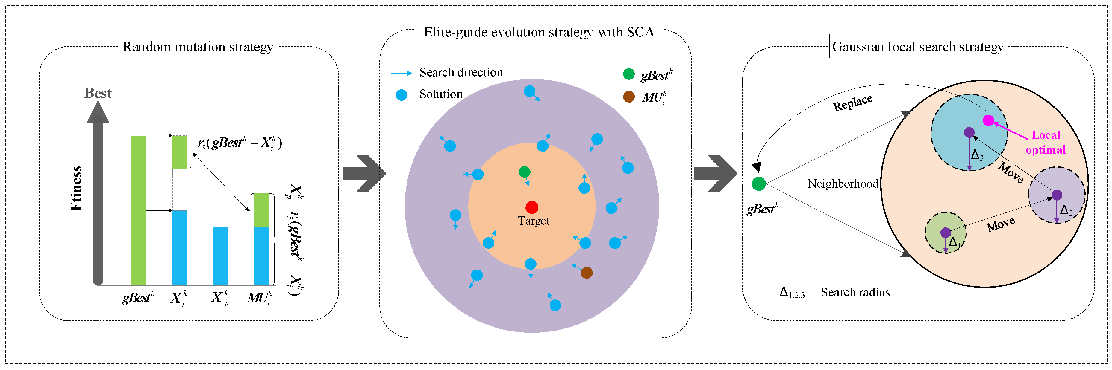
2.3. Elite-Guide Evolution Strategy to Improve the Convergence Speed

Generally, the global optima are the best position found by the swarm from the beginning to the current cycle. When the individuals search in the neighborhoods of the global optima, it is possible to find a solution with better performance [44,45,46]. Thus, the elite-guide evolution strategy is proposed to improve the convergence rate of the population. The combined individual balancing the current individual and the global optima is firstly generated, and then the positions of all the individuals are dynamically updated to improve the converged rate. Then, the above analysis can be expressed as:
X i k + 1 = { M i k + r 1 × sin ( r 2 ) × | r 3 × g B e s t k X i k | if ( r 4 < 0.5 ) M i k + r 1 × cos ( r 2 ) × | r 3 × g B e s t k X i k | otherwise
M i k = a × X i k + ( 1 a ) × g B e s t k
where M i k is the position of the ith combined individual at the kth iteration. a is the combination coefficient in the range of [0,1].

2.4. Gaussian Local Search Strategy to Improve the Individuals’ Search Capability

As mentioned above, it is possible to find a better position around the global optimal individual in the evolution process [47,48,49,50]. Therefore, the Gaussian local search strategy in Figure 1 is used to improve the individuals’ performance. Based on the Gaussian distribution, a random perturbation is employed to generate a Gaussian individual around the global optima, and then the greedy selection is used to ensure that the better solution is chosen, which can help the swarm jump out of local optima and improve the convergence rate. Then, the Gaussian local search strategy can be expressed as:
B k = g B e s t k × ( 1 + Gauss ( 0 , 1 ) )
g B e s t k = { B k if { F ( B k ) < F ( g B e s t k ) } g B e s t k otherwise
where Gauss ( 0 , 1 ) is the random number obeying the Gaussian distribution. B k is the position of the Gaussian individual at the kth iteration.

2.5. Random Mutation Strategy to Increase the Population Diversity

Similar to the other evolutionary methods, the SCA method is often trapped into local optima because the population diversity gradually decreases during the evolution process [51]. Hence, it is important to find some strategies that can help individuals search in different directions [52,53]. To achieve this goal, a novel random mutation strategy is proposed to effectively increase the diversity of the swarm. Firstly, the global optimal solution is used to generate a mutant individual for each individual so as to provide multiple search directions. Then the parent solution will be replaced by the mutant individual when certain criteria is satisfied. Figure 2 shows the sketch map of the random mutation strategy, which can be expressed as follows:
M U i k = X p k + r 5 × ( g B e s t k X i k )
X i k = { M U i k if { F ( M U i k ) < F ( X i k ) }   or   { F ( M U i k ) < F ¯   and   r 6 < P x } X i k otherwise
where M U i k is the position of the ith mutant individual at the kth iteration. P x is the preset mutation probability, p is the index randomly selected from the set of { 1 , 2 , , I } . r 5 and r 6 are two random numbers in the range of [ 0 , 1 ] . F ¯ is the average fitness value of all the individuals in the current population.

2.6. Execution Procedure of the Proposed HSCA Method

In the HSCA algorithm, three modified strategies are used to improve the performance of the standard SCA method in high-dimensional and multi-constraint problems, including the convergence speed, swarm diversity and solution stability. Figure 3 shows the sketch map of the HSCA algorithm while Table 1 shows the execution procedures of the HSCA method. It can be found that firstly, the SCA method can help individuals search in the problem space. Secondly, the random mutation strategy is used to generate the mutant solutions and replace the poor quality individuals with a certain probability. Finally, the Gaussian local search strategy is used to enhance the exploration capabilities as well as the quality of the global optimal position in the current swarm.

3. Numerical Experiments to Verify the Feasibility of the HSCA Method

In this section, six classical benchmark functions were used to testify the performance of HSCA, while four classic algorithms were introduced for comparative analysis.

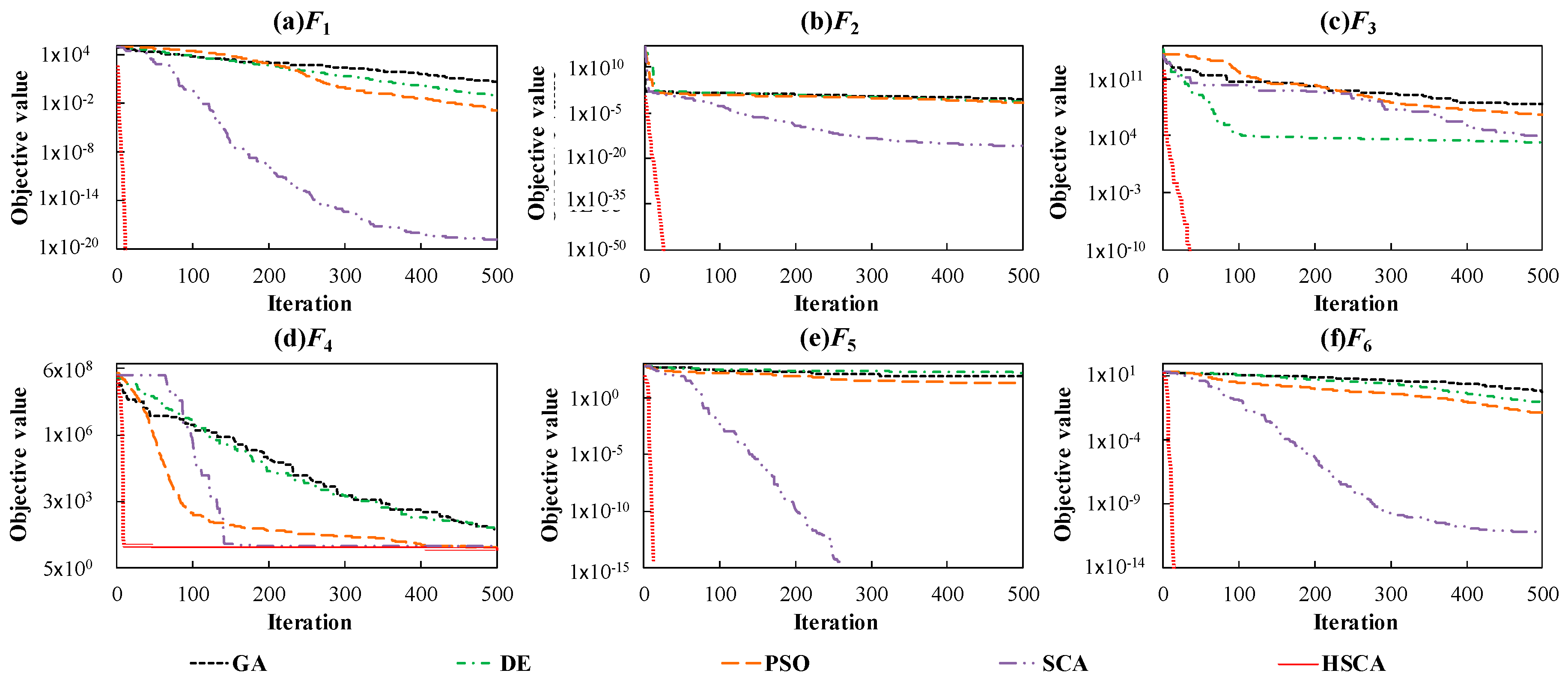
3.1. Benchmark Functions

In this section, six famous benchmark functions in Ref [54] are employed to test the feasibility of the HSCA method. Table 2 shows the detailed information of test functions. The selected benchmark functions can be roughly classified into two different groups, unimodal functions (F1F4) used to test the convergence ability and multimodal functions (F5F6) used to testify the ability of jumping out of local optima.

3.2. Parameter Settings

Here, four methods are introduced for comparison and analysis, including genetic algorithm, differential evolution algorithm, particle swarm optimization algorithm and sine cosine algorithm. For the sake of comparison, the swarm size and maximum iterations of four algorithms are set to 50 and 500 based on numerical experiments. Besides, the other parameters are defined as:
HSCA: The combination coefficient a and mutation probability Px are set to 0.5 and 0.01.
GA: The crossover probability and mutation probability are set to 0.6 and 0.2, respectively.
DE: The crossover probability and scaling factor are set to be 0.8 and 0.5, respectively.
PSO: The inertia weight (w) is decreased linearly from the initial value 0.9 to the final value 0.4, while the values of two learning factors (c1 and c2) are set as 2.0, respectively.

3.3. Performances of the HSCA Method

Table 3 and Table 4 show the statistical indexes of the objective values obtained by different algorithms in 30 independent runs for the benchmark functions with 40 and 80 variables, including the best, average and standard deviation. Figure 4 and Figure 5 show the convergence trajectories of five algorithms for 6 benchmark functions, where the number of decision variables are set as 40 and 80, respectively.
The data listed in Table 3 and Table 4 show that HSCA achieves better results than four other methods. Especially in the experiments of three benchmark functions (F1, F2 and F5), HSCA is able to find the optimal objective value. For three other functions (F3, F4 and F6), HSCA can still seek out the best solutions among all the methods, demonstrating the feasibility of the developed modified strategies in enhancing the SCA performance. From Figure 4 and Figure 5, it can be seen that for three functions (F1, F5 and F6), the search abilities of GA and DE gradually become poor. PSO using historical memory of individuals and swarm can obtain better results than GA and DE but is still inferior to HSCA. The convergence rate of SCA outperforms three other methods. For F3 and F4, DE and SCA produce satisfying performances at the initial phase, while the advantage of PSO gradually emerges as the search process increases. Meanwhile, the convergence rate of HSCA always stands out among five algorithms regardless of the function form. Thus, it can be concluded that the modified strategies can effectively accelerate the convergence rate and search capability, and HSCA is a feasible tool for solving global optimization problems.

4. HSCA for the Peak Operation of Cascade Hydropower Reservoirs

In this section, the details of the HSCA method for the peak operation of cascade hydropower reservoirs are given, like the optimization model, swarm initialization and the constraint handling method.

4.1. Mathematical Model

4.1.1. Objective Function

As mentioned above, the dynamic balance between load demand and energy consumption at peak periods is posing an enormous challenge for operators in electric power systems. Thus, the goal of this paper is chosen to determine the scheduling process of all the hydropower plants to obtain a smooth residual load curve, which can be expressed as below:
min F = 1 2 t = 1 T [ L t n = 1 N P n , t ] 2
where T is the number of periods. Lt is the load demand of the power system at tth period. N is the number of hydropower reservoirs. Pn,t is the output of nth hydropower plant at tth period.

4.1.2. Operation Constraints

In the modeling process, the following equality and inequality constraints should be strictly satisfied to guarantee the safe operation of power system in the entire scheduling horizon [55,56,57,58].
(1) Water balance equation:
V n , t + 1 = V n , t + [ I n , t + j = 1 N U n ( Q j , t + S j , t ) Q n , t S n , t ] Δ t
where NUn is the number of upstream reservoirs directly connected to the nth reservoir. V n , t = f n ( Z n , t ) , In,t, Qn,t and Sn,t are the storage volume, local flow, turbine discharge and spillage of the nth reservoir at the tth period. f n ( · ) denotes the nonlinear relationship between forebay water level and storage volume of the nth reservoir. Z n , t is the forebay water level of the nth reservoir at the tth period.
(2) Water level constraint:
Z n , t d o w n Z n , t Z n , t u p
where Z n , t d o w n and Z n , t u p are the minimum and maximum forebay water levels of the nth reservoir at the tth period, respectively.
(3) Turbine discharge constraints:
q n , t d o w n q n , t q n , t u p
where q n , t d o w n and q n , t u p are the minimum and maximum turbine discharges of the nth reservoir at the tth period, respectively.
(4) Power output constraints:
P n , t d o w n P n , t P n , t u p
where P n , t d o w n and P n , t u p are the minimum and maximum power outputs of the nth reservoir at the tth period, respectively.
(5) Total output constraints:
L t d o w n n = 1 N P n , t L t u p
where L n , t d o w n and L n , t u p are the minimum and maximum total outputs of hydropower system at the tth period, respectively.
(6) Initial and final water levels constraints:
{ Z n , 0 = Z n b e g i n Z n , T = Z n e n d
where Z n b e g i n and Z n e n d are the initial and final water levels of the nth reservoir, respectively.

4.2. Details of HSCA for Peak Operation of Cascade Hydropower Reservoirs

4.2.1. Individual Encoding and Swarm Initiation Strategies

When solving the peak operation problem of cascade hydropower reservoirs, the appropriate decision variable will be useful to accelerate the execution efficiency of the algorithm. Here, the decision variables are chosen as the total discharges of each hydropower reservoir that can be used to obtain the detailed scheduling processes (like output and water level). Then, the elements for the ith individual at the kth iteration can be described as below:
X i k = [ q 1 , 1 , q 1 , 2 , , q 1 , T , q n , t , , q N , 1 , q N , 2 , , q N , T ]
In the initialization stage, the decision variable qn,t of each hydropower reservoir is randomly generated in the feasible range between q n , t d o w n and q n , t u p ,which can be described as follows:
q n , t = q n , t d o w n + R a n d o m × ( q n , t u p q n , t d o w n )
where Random is the random number in the range of [0,1].

4.2.2. Constraint Handling Method

Due to plenty of physical constraints in practice, some individuals may fall into the infeasible zones during the evolutionary process [53,59]. To address this case, an effective constraint handling method based on penalty coefficient and heuristic modification strategies is proposed, where the variables violating the feasible zone are forced to be the boundary range, and then the constraint violation is merged into the objective function. The detailed procedure for solution X i k is as below:
Step 1: Set n = 0 and start the constraint handling process.
Step 2: Set n = n + 1 . If n > N , turn to Step 7, otherwise go to Step 3 to deal with the constraints of the nth hydropower reservoir.
Step 3: Define the counter c = 1. The total discharges q n , t are substituted into the water balance equation to calculate the feasible storages, which can be expressed as below:
V n , t = max { V n , t d o w n , min { V n , t 1 + [ I n , t 1 + j = 1 N U n ( Q j , t 1 + S j , t 1 ) Q n , t 1 S n , t 1 ] Δ t 1 , V n , t u p } }
Step 4: Set c = c + 1 . Calculate the difference Δ V between the obtained final storage V n , T and the predetermined terminal storage V n e n d . If Δ V is smaller than the minimum accuracy μ or c exceeds the constraint adjustment time c max , go to Step 6, otherwise go to Step 5.
Δ V = V n , T V n e n d
Step 5: Use Equation (24) to calculate the modified total discharges in the feasible range. Then, Equation (22) is used to recalculate the corresponding reservoir storage volume before going back to Step 4.
q n , t = max { q n , t d o w n , min { q n , t + Δ V T × t = 1 T Δ t , q n , t u p } }
Step 6: Record the outputs and constraint violations of the nth reservoir and turn to Step 2.
Step 7: Calculate the objective function and constraint violation values for the target solution, which can be described as below:
F ( X i k ) = 1 2 t = 1 T [ L t n = 1 N P n , t ] 2 + j = 1 J λ j A j
where F ( X i k ) is the fitness value of solution X i k . J is the number of constraints. λ j and Aj are the penalty factor and constraint violation value of the jth constraint, respectively.

4.2.3. Overall Execution Procedures

The execution procedure of HSCA for the peak operation of cascade hydropower reservoirs is given in Figure 6.

5. Case Studies

In this section, the HSCA method was applied to determine the optimal scheduling process of two multi-reservoir hydropower systems, and the detailed procedures are given in Section 4.2. In the first hydropower system, it is assumed that there are linear relationships and no units in the characteristic curves to reduce the modeling complexity. In the second hydropower system, all the prototype physical constraints are used to verify the practicality of the developed methods.

5.1. Mature Multi-Reservoir System

In this section, the mature multi-reservoir system problem is used to verify the feasibility of the proposed method. The topology of the multi-reservoir system is shown in Figure 7, while basic information can be found in Table 5 and Table 6. It is to be mentioned that the storage capacity changes of the 7th and 10th reservoirs are larger than those of other reservoirs. Then, five swarm-based methods mentioned in Section 3.2. are introduced for comparison. To guarantee the computational efficiency, the swarm size and maximal iterations are set as 50 and 200 for the mature multi-reservoir system. To avoid the possible solution randomness problem, four cases with different final storages in Table 7 are used for testing, and each method is independently executed 20 times.

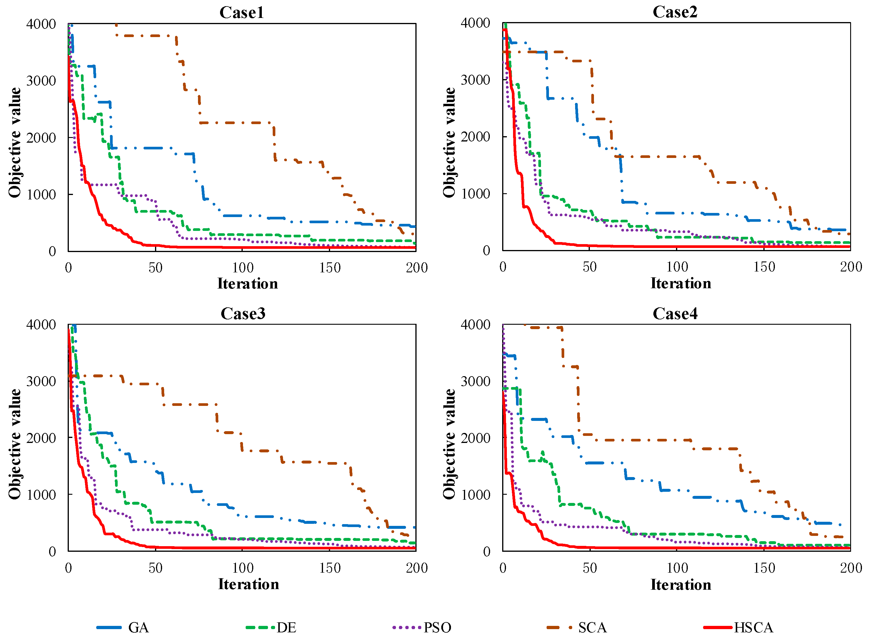
5.1.1. Convergence Process Analysis

The convergence trajectories of five methods in four cases with different terminal storages are drawn in Figure 8. It can be found that as the iteration processes, the performances of DE and GA are gradually improved and the objective values of PSO and SCA change slightly, which means that the four methods are lacking search ability for the multi-constrained reservoir operation problems. On the other hand, the objective values of the HSCA method always outperform the other algorithms from beginning to end, while the entire search process presents a smooth decline trend at the early stage. Thus, it can be concluded that the proposed method has strong search efficiency in solving the high-dimensional cascade reservoir operation problem.

5.1.2. Simulation and Result Analysis

Figure 9 shows the optimal objective values of five algorithms for four cases. It can be seen that the objective value of the proposed HSCA algorithm is the best in different cases. In the comparison of SCA, the objective values are reduced by about 240.64, 225.65, 195.98, and 191.66, respectively. Thus, HSCA has strong search ability in the peak operation of cascade hydropower reservoirs.

5.1.3. Robustness Performance of the HSCA Method

Figure 10 shows the box plots of five methods obtained in 100 independent runs for the mature hydropower system in four cases. The box plots are composed of the lower quartile, the median, the upper quartile, the upper and lower limits of the objective values, where the median is the number in the middle position in ascending order. In general, the stability of the dispersive box plot is poor. From Figure 10, it can be found that in four cases, GA and SCA show a relatively large distribution. The distributions of PSO and DE are relatively small, while HSCA shows a highly concentrated distribution. Besides, similar results between PSO and HSCA can be observed, and the reasons are analyzed as follows. Several modified strategies contribute to the best search ability of the HSCA method. In the evolutionary model of PSO, the tendency following preceding velocity and the impacts of the personal best and global best solution are simultaneously considered, making it have better performance than GA and SCA. Thus, this case fully demonstrates that although the initial swarm is generated from different random seeds, the developed HSCA method always achieves stable results in reducing the peak loads of power systems.

5.2. Real-World Multi-Reservoir System

5.2.1. Engineering Background

In this section, five reservoirs located in the mainstream of the Wu River in China are selected to further test the performance of the HSCA method, including Hongjiadu (HJD), Dongfeng (DF) and Suofengying (SFY), Wujiangdu (WJD) and Goupitan (GPT). Wu River is regarded as one of the most important hydropower bases and plays an important role in boosting the economic development of Guizhou province in southwest China. Figure 11 and Table 8 show the topological structure and basic information of the studied hydropower reservoirs, respectively. Next, the five methods in Section 3.2. are employed for comparison. To balance the computational accuracy and execution time, the swarm size and maximal iterations are set as 150 and 500. The scheduling horizon is set as 1 day with 24 identical intervals.

5.2.2. Simulation and Analysis of the HSCA Method

Table 9 shows the real-world simulation results of five algorithms in spring. From Table 9, it can be found that HSCA can get better results than four other methods in terms of all the statistical indexes. For instance, as compared with GA, DE, PSO and SCA, the peak loads in the optimization results of the HSCA method are reduced by about 1300.82, 628.00, 190.85, 1148.04 MW, respectively. Obviously, the proposed method can obtain smoother residual load curves and stand out among the compared algorithms.
Table 10 shows the optimization results of the HSCA algorithm in different load requirements. The data in Table 10 shows that HSCA can achieve satisfying scheduling results in three seasons. For instance, compared with the original loads, the peak values of the residual loads obtained by HSCA was improved by 26.79%, 21.68% and 25.71%, while the average standard deviations are reduced by more than 80%. Thus, this case fully demonstrates that HSCA can undertake the peak operation task of the real-world hydropower system in practice.
To further show the solution rationality, Figure 12 shows the best scheduling results obtained by the HSCA method for the Wu hydropower system in four seasons. For the original load curve in four seasons, the loads in the valley periods are relatively stable at the beginning and then increase at both morning and evening peak periods. Obviously, for the optimization method, it becomes much more difficult to find the feasible scheduling solution due to the fast changing characteristic of the energy load curve. The HSCA method can collect hydropower generation during peak periods to respond to the load change and decrease the outputs during valley periods to store energy in reservoirs. In the hydropower system, HJD mainly undertakes the peak operation tasks at the early stages. The outputs of three downstream reservoirs (DF, SFY and WJD) show a relatively stable trend, while GPT plays an important role in providing generation at the later stages. In this way, the satisfactory residual loads are produced in four cases with varying load requirements. Thus, it can be concluded that HSCA has strong capability in solving the hydropower peak operation problem with multiple spatial–temporal coupling constraints.
In the HSCA method, six computational parameters may have certain effects on the optimized results. The orthogonal experiment design is used to test the role of six parameters [58]. Table 11 shows the results of the HSCA method with different parameter combinations in summer. In Table 11, the level denotes the possible value of the target parameter (the swarm sizes in level 1~3 are 100, 150 and 200), while the objective value denotes the average value of the standard deviation of the HSCA method in five independent runs. It can be found that the maximum iterations and the constraint adjustment time have the greatest influence on the final result. The reasons lie in that two parameters with larger values can effectively help the swarm produce feasible solutions with better objective values during the evolutionary process. Thus, the computation parameters have different effects on the objective value obtained by the HSCA method, and it is of great significance to carefully choose the parameter combination based on the characteristics of engineering problems in practice.

5.2.3. Robustness Performance of the HSCA Method

Figure 13 shows the box plot of five algorithms in different seasons, where the results of each method are obtained in 20 independent runs where the initial swarm per run is generated from a newly obtained random seed. As showed in Figure 13, although three methods (GA, DE and SCA) exhibit satisfying stability in the peak operation of hydropower systems, the results of the HSCA method have the best performance due to the smallest fluctuation in the objective function. Thus, this case proves that from different initial swarms, HSCA can generate a stable scheduling process for high-dimensional and multi-constrained engineering problems.
Figure 14 shows the results of the remaining electrical loads obtained by three methods in four seasons, where the difference represents the maximum peak load minus the minimum valley load. As shown in Figure 14, there are no obvious differences in the average loads of SCA and HSCA, but the peak-valley differences and standard deviations of HSCA are much smaller than SCA. Generally, the smaller values of the peak-valley difference and standard deviation denote a smoother load series [60]. Therefore, it can be concluded that the HSCA approach has a stronger optimization ability in using the hydropower generation to reduce the peak loads of the power system.

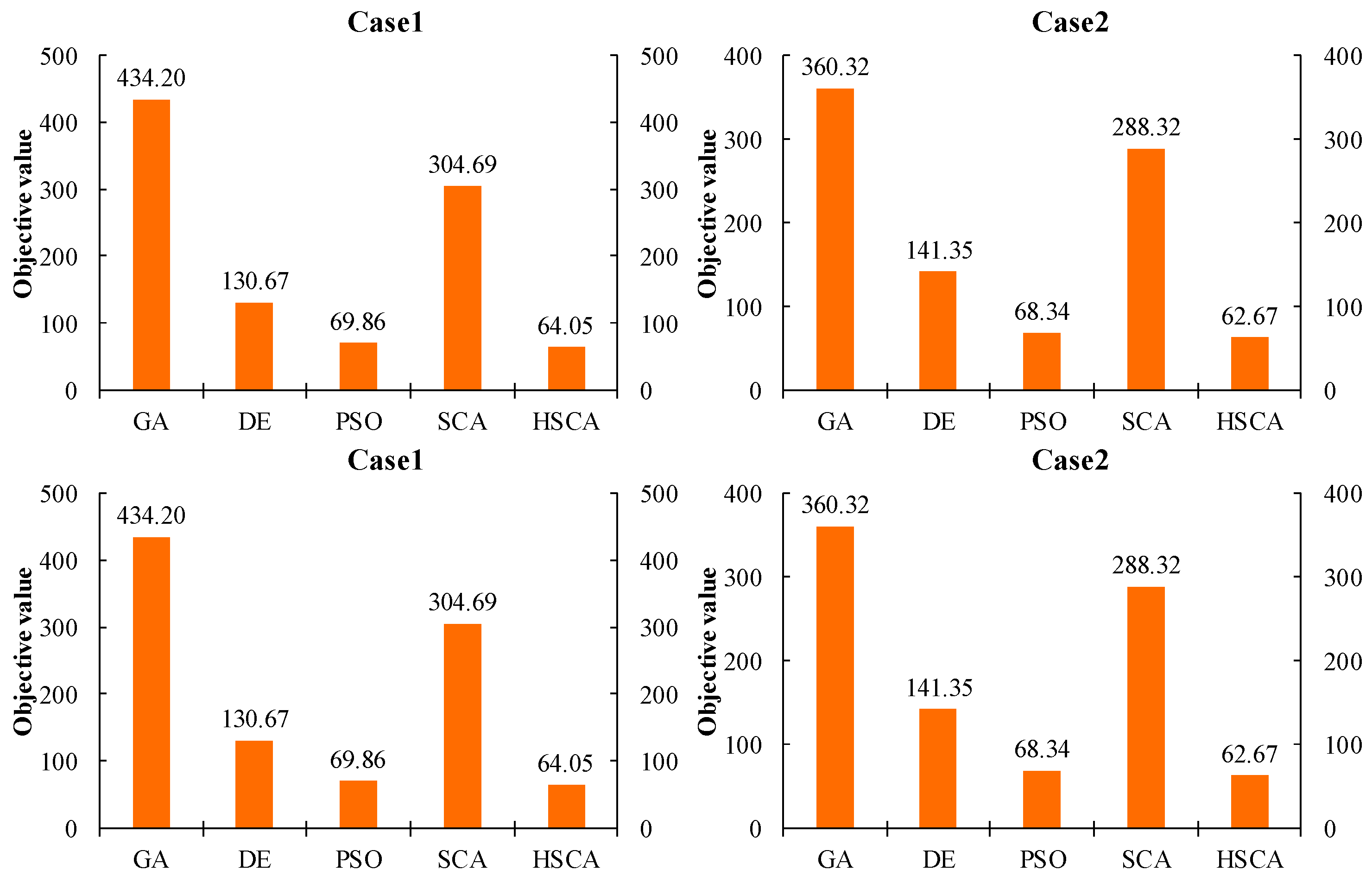
5.2.4. Performances of the HSCA Method in Different Cases

Table 12 shows the statistical results of different algorithms in 12 cases where the operation conditions (like local inflow and load demand) per case are different, including the peak load, peak-valley difference, standard deviation and load rate. Figure 15 shows the hydropower output and residual loads obtained by HSCA and SCA. From the data listed in Table 12, it can be found that the results obtained by the SCA algorithm in 12 cases are inferior to HSCA since the peak-valley difference and peak load are improved by about 300 MW and 700 MW, while the average load rates are increased by about 96%. This fully demonstrates that HSCA can solve the complex hydropower peak operation problem. Meanwhile, from Figure 15, it can be found that the residual loads obtained by SCA are unstable in the scheduling horizon, while the hydropower outputs of HSCA can respond to the load change in a better way and a smoother residual load curve is left for other energy sources represented by thermal plants. Thus, this case proves that the HSCA method has a strong ability to satisfy the peak loads of the power system under uncertainty.

5.3. Result Discussion

From the above simulated results, it can be clearly found that the developed method has better performances than several benchmark methods (like GA, PSO and SCA). The standard GA method uses the crossover, selection and mutation operators to simulate the survival of the fittest in nature, and the parameter choices of three operators and the quality of the initial swarm have an important effect on the final solution. In the standard PSO method, each potential solution is seen as a particle with velocity and position vectors, and all the particles tend to fall into the neighborhood of the best-known solution of the swarm due to the loss of population diversity. In the SCA method, the sine and cosine functions are employed to guide the evolutionary process while the role of elitist individuals is ignored at a certain degree, resulting in the premature convergence problem. On the other hand, several modified strategies are helpful to guarantee the superior performance of the developed HSCA method. Firstly, the elite-guide strategy embedded in the updating equation of the standard method takes full use of the elitist individuals to provide multiple search directions, which can effectively enhance the convergence rate of the swarm in the evolutionary process. Secondly, the Gaussian local search strategy is used to generate a temporary solution for the global best-known position, which can dynamically update the shared knowledge of the swarm and then improve the search ability of all the individuals. Thirdly, the random mutation strategy is used to provide the chance to improve the solution quality for each individual, which can increase the diversity of the swarm and avoid falling into local optima. Finally, the heuristic constraint handling method can iteratively adjust the scheduling processes of all the hydropower reservoirs from upstream to downstream, which can alleviate the negative effects of the infeasible solutions. In this way, the HSCA algorithm is able to produce solutions with higher quality in different cases as used to handle the peak operation of cascade hydropower reservoirs. Besides, it can be implied that the solution quality of the evolutionary algorithms can be improved by incorporating multiple beneficial strategies in the iterative search process [56,61,62], which can provide technical reference for similar engineering problems.

6. Conclusions

In recent years, the peak operation of cascade hydropower reservoirs is posing a great challenge for operators in China’s electrical power system. As a brand new evolutionary method, the sine cosine algorithm (SCA) has not been applied in the hydropower operation field. In order to fill this gap, the performance of the SCA method is tested in the studied engineering problem for the first time, but it was found that the standard SCA method still suffers from the premature convergence problem. Thus, for the sake of improving the SCA performance, this research develops a hybrid sine cosine algorithm (HSCA) linking the merits of several modified strategies into SCA. The HSCA method is applied to solve several test functions and the hydropower peak operation problems. The following conclusions can be deduced from the experimental results: (1) due to the premature convergence problem, the standard SCA, GA and PSO methods have poor performances in the peak operation of cascade hydropower reservoirs, (2) the HSCA method can obtain better solutions by reasonably allocating hydropower generation in the scheduling horizon, where the elite-guide evolution strategy, Gaussian local search strategy and random mutation operator can effectively improve the convergence speed and search ability of the swarm, (3) a practical constraint handling strategy is proposed to guarantee the solutions’ quality in the evolutionary process. Thus, a feasible tool is provided to solve the peak operation of cascade hydropower reservoirs.
It should be mentioned that even though the feasibility of the developed method is verified in this study, there are still some shortcomings deserving attention. One is the inevitable premature convergence problem rooted in evolutionary algorithms. The other is the practicality of the constraint handling technique in the elaborate management of cascade hydropower reservoirs where more complex spatial–temporal coupling constraints need to be considered. Hence, in the future, the research can be carried out in two aspects. The first is to enhance the global search ability of the HSCA method by developing more effective strategies or introducing new ideas from other methods. The other is to develop more practical constraint handling tools based on the actual characteristics of the target engineering problems.

Author Contributions

All authors contributed extensively to the work of this paper. S.L. contributed to the modeling. Z.-K.F. and W.-J.N. finalized the manuscripts. H.-R.Z. contributed to the data analysis, while Z.-G.S. contributed to the literature review.

Acknowledgments

This study is supported by the National Key R&D Program of China (2017YFC0405900), National Natural Science Foundation of China (51709119), the Natural Science Foundation of Hubei Province (2018CFB573), and Fundamental Research Funds for the Central Universities (HUST: 2017KFYXJJ193). The writers would like to thank editors and reviewers for their valuable comments and suggestions.

Conflicts of Interest

The authors declare no conflict of interest.

References

  1. Feng, Z.K.; Niu, W.J.; Cheng, C.T. China’s large-scale hydropower system: Operation characteristics, modeling challenge and dimensionality reduction possibilities. Renew. Energy 2019, 136, 805–818. [Google Scholar] [CrossRef]
  2. Cheng, C.; Shen, J.; Wu, X.; Chau, K. Operation challenges for fast-growing China’s hydropower systems and respondence to energy saving and emission reduction. Renew. Sustain. Energy Rev. 2012, 16, 2386–2393. [Google Scholar] [CrossRef]
  3. Yu, L.; Li, Y.P.; Huang, G.H. A fuzzy-stochastic simulation-optimization model for planning electric power systems with considering peak-electricity demand: A case study of Qingdao, China. Energy 2016, 98, 190–203. [Google Scholar] [CrossRef]
  4. Yu, L.; Li, Y.P.; Huang, G.H.; An, C.J. A robust flexible-probabilistic programming method for planning municipal energy system with considering peak-electricity price and electric vehicle. Energy Convers. Manag. 2017, 137, 97–112. [Google Scholar] [CrossRef]
  5. Feng, Z.; Niu, W.; Wang, W.; Zhou, J.; Cheng, C. A mixed integer linear programming model for unit commitment of thermal plants with peak shaving operation aspect in regional power grid lack of flexible hydropower energy. Energy 2019, 175, 618–629. [Google Scholar] [CrossRef]
  6. Xu, B.; Zhong, P.A.; Wan, X.; Zhang, W.; Chen, X. Dynamic feasible region genetic algorithm for optimal operation of a multi-reservoir system. Energies 2012, 5, 2894–2910. [Google Scholar] [CrossRef]
  7. Chen, D.; Liu, S.; Ma, X. Modeling, nonlinear dynamical analysis of a novel power system with random wind power and it’s control. Energy 2013, 53, 139–146. [Google Scholar] [CrossRef]
  8. Niu, W.J.; Feng, Z.K.; Feng, B.F.; Min, Y.W.; Cheng, C.T.; Zhou, J.Z. Comparison of multiple linear regression, artificial neural network, extreme learning machine, and support vector machine in deriving operation rule of hydropower reservoir. Water 2019, 11, 88. [Google Scholar] [CrossRef]
  9. Dehghani, M.; Riahi-Madvar, H.; Hooshyaripor, F.; Mosavi, A.; Shamshirband, S.; Zavadskas, E.K.; Chau, K.W. Prediction of hydropower generation using grey Wolf optimization adaptive neuro-fuzzy inference system. Energies 2019, 12, 289. [Google Scholar] [CrossRef]
  10. Zhou, J.; Xu, Y.; Zheng, Y.; Zhang, Y. Optimization of guide vane closing schemes of pumped storage hydro unit using an enhanced multi-objective gravitational search algorithm. Energies 2017, 10, 911. [Google Scholar] [CrossRef]
  11. Ji, C.; Li, C.; Wang, B.; Liu, M.; Wang, L. Multi-Stage dynamic programming method for Short-Term cascade reservoirs optimal operation with flow attenuation. Water Resour. Manag. 2017, 31, 4571–4586. [Google Scholar] [CrossRef]
  12. Ye, L.; Ding, W.; Zeng, X.; Xin, Z.; Wu, J.; Zhang, C. Inherent relationship between flow duration curves at different time scales: A perspective on monthly flow data utilization in daily flow duration curve estimation. Water 2018, 10, 1008. [Google Scholar] [CrossRef]
  13. Ding, W.; Zhang, C.; Peng, Y.; Zeng, R.; Zhou, H.; Cai, X. An analytical framework for flood water conservation considering forecast uncertainty and acceptable risk. Water Resour. Res. 2015, 51, 4702–4726. [Google Scholar] [CrossRef]
  14. Feng, Z.K.; Niu, W.J.; Cheng, C.T.; Zhou, J.Z. Peak shaving operation of hydro-thermal-nuclear plants serving multiple power grids by linear programming. Energy 2017, 135, 210–219. [Google Scholar] [CrossRef]
  15. Madani, K.; Lund, J.R. Modeling California’s high-elevation hydropower systems in energy units. Water Resour. Res. 2009, 45, W09413. [Google Scholar] [CrossRef]
  16. Madani, K. Game theory and water resources. J. Hydrol. 2010, 381, 225–238. [Google Scholar] [CrossRef]
  17. Zhao, J.; Cai, X.; Wang, Z. Optimality conditions for a two-stage reservoir operation problem. Water Resour. Res. 2011, 47, W08503. [Google Scholar] [CrossRef]
  18. Liu, J.; Li, Y.P.; Huang, G.H.; Zeng, X.T. A dual-interval fixed-mix stochastic programming method for water resources management under uncertainty. Resour. Conserv. Recycl. 2014, 88, 50–66. [Google Scholar] [CrossRef]
  19. Zhao, T.; Zhao, J.; Liu, P.; Lei, X. Evaluating the marginal utility principle for long-term hydropower scheduling. Energy Convers. Manag. 2015, 106, 213–223. [Google Scholar] [CrossRef] [Green Version]
  20. Guo, S.; Chen, J.; Li, Y.; Liu, P.; Li, T. Joint operation of the multi-reservoir system of the Three Gorges and the Qingjiang cascade reservoirs. Energies 2011, 4, 1036–1050. [Google Scholar] [CrossRef]
  21. Feng, Z.K.; Niu, W.J.; Wang, S.; Cheng, C.T.; Jiang, Z.Q.; Qin, H.; Liu, Y. Developing a successive linear programming model for head-sensitive hydropower system operation considering power shortage aspect. Energy 2018, 115, 252–261. [Google Scholar] [CrossRef]
  22. Feng, Z.K.; Niu, W.J.; Cheng, C.T.; Wu, X.Y. Optimization of hydropower system operation by uniform dynamic programming for dimensionality reduction. Energy 2017, 134, 718–730. [Google Scholar] [CrossRef]
  23. Zheng, F.; Simpson, A.R.; Zecchin, A.C. A combined NLP-differential evolution algorithm approach for the optimization of looped water distribution systems. Water Resour. Res. 2011, 47, W08531. [Google Scholar] [CrossRef]
  24. Bai, T.; Kan, Y.B.; Chang, J.X.; Huang, Q.; Chang, F.J. Fusing feasible search space into PSO for multi-objective cascade reservoir optimization. Appl. Soft Comput. J. 2017, 51, 328–340. [Google Scholar] [CrossRef]
  25. Ma, C.; Lian, J.; Wang, J. Short-term optimal operation of Three-gorge and Gezhouba cascade hydropower stations in non-flood season with operation rules from data mining. Energy Convers. Manag. 2013, 65, 616–627. [Google Scholar] [CrossRef]
  26. Cai, X.; McKinney, D.C.; Lasdon, L.S. Solving nonlinear water management models using a combined genetic algorithm and linear programming approach. Adv. Water Resour. 2001, 24, 667–676. [Google Scholar] [CrossRef]
  27. Feng, Z.K.; Niu, W.J.; Cheng, C.T. Optimization of hydropower reservoirs operation balancing generation benefit and ecological requirement with parallel multi-objective genetic algorithm. Energy 2018, 153, 706–718. [Google Scholar] [CrossRef]
  28. Osório, G.J.; Gonçalves, J.N.D.L.; Lujano-Rojas, J.M.; Catalão, J.P.S. Enhanced forecasting approach for electricity market prices and wind power data series in the short-term. Energies 2016, 9, 693. [Google Scholar] [CrossRef]
  29. Feng, Z.K.; Niu, W.J.; Cheng, C.T. Multi-objective quantum-behaved particle swarm optimization for economic environmental hydrothermal energy system scheduling. Energy 2017, 131, 165–178. [Google Scholar] [CrossRef]
  30. Vašcák, J. Adaptation of fuzzy cognitive maps by migration algorithms. Kybernetes 2012, 41, 429–443. [Google Scholar] [CrossRef] [Green Version]
  31. Shams, M.; Rashedi, E.; Dashti, S.M.; Hakimi, A. Ideal gas optimization algorithm. Int. J. Artif. Intell. 2017, 15, 116–130. [Google Scholar]
  32. Vrkalovic, S.; Lunca, E.-C.; Borlea, I.-D. Model-free sliding mode and fuzzy controllers for reverse osmosis desalination plants. Int. J. Artif. Intell. 2018, 16, 208–222. [Google Scholar]
  33. Precup, R.E.; David, R.C. Nature-Inspired Optimization Algorithms for Fuzzy Controlled Servo Systems; Butterworth-Heinemann: Oxford, UK, 2019. [Google Scholar]
  34. Wang, J.; Yang, W.; Du, P.; Niu, T. A novel hybrid forecasting system of wind speed based on a newly developed multi-objective sine cosine algorithm. Energy Convers. Manag. 2018, 163, 134–150. [Google Scholar] [CrossRef]
  35. Gupta, S.; Deep, K. A hybrid self-adaptive sine cosine algorithm with opposition based learning. Expert Syst. Appl. 2019, 119, 210–230. [Google Scholar] [CrossRef]
  36. Abd Elaziz, M.; Oliva, D.; Xiong, S. An improved Opposition-Based Sine Cosine Algorithm for global optimization. Expert Syst. Appl. 2017, 90, 484–500. [Google Scholar] [CrossRef]
  37. Li, S.; Fang, H.; Liu, X. Parameter optimization of support vector regression based on sine cosine algorithm. Expert Syst. Appl. 2018, 91, 63–77. [Google Scholar] [CrossRef]
  38. Fu, W.; Tan, J.; Li, C.; Zou, Z.; Li, Q.; Chen, T. A hybrid fault diagnosis approach for rotating machinery with the fusion of entropy-based feature extraction and SVM optimized by a chaos quantum sine cosine algorithm. Entropy 2018, 20, 626. [Google Scholar] [CrossRef]
  39. Yuan, X.; Tian, H.; Yuan, Y.; Zhang, X. Multi-objective artificial physical optimization algorithm for daily economic environmental dispatch of hydrothermal systems. Electr. Power Compon. Syst. 2016, 44, 533–543. [Google Scholar] [CrossRef]
  40. Lai, X.; Li, C.; Zhang, N.; Zhou, J. A multi-objective artificial sheep algorithm. Neural Comput. Appl. 2018, 1–35. [Google Scholar] [CrossRef]
  41. Rizk-Allah, R.M. Hybridizing sine cosine algorithm with multi-orthogonal search strategy for engineering design problems. J. Comput. Des. Eng. 2018, 5, 249–273. [Google Scholar] [CrossRef]
  42. Gupta, S.; Deep, K. Improved sine cosine algorithm with crossover scheme for global optimization. Knowl. Based Syst. 2019, 165, 374–406. [Google Scholar] [CrossRef]
  43. Nenavath, H.; Kumar Jatoth, D.R.; Das, D.S. A synergy of the sine-cosine algorithm and particle swarm optimizer for improved global optimization and object tracking. Swarm Evol. Comput. 2018, 43, 1–30. [Google Scholar] [CrossRef]
  44. Zhang, R.; Zhou, J.; Ouyang, S.; Wang, X.; Zhang, H. Optimal operation of multi-reservoir system by multi-elite guide particle swarm optimization. Int. J. Electr. Power Energy Syst. 2013, 48, 58–68. [Google Scholar] [CrossRef]
  45. Mu, C.; Jiao, L.; Liu, Y.; Li, Y. Multiobjective nondominated neighbor coevolutionary algorithm with elite population. Soft Comput. 2015, 19, 1329–1349. [Google Scholar] [CrossRef]
  46. Li, Z.; Tan, H.; Zhang, Y. Efficient artificial immune network with elite-learning inspired from PSO for optimization. J. Comput. Inf. Syst. 2008, 4, 1331–1338. [Google Scholar]
  47. Chang, J.X.; Huang, Q.; Wang, Y.M. Genetic algorithms for optimal reservoir dispatching. Water Resour. Manag. 2005, 19, 321–331. [Google Scholar]
  48. Coelho, L.D.S. Gaussian quantum-behaved particle swarm optimization approaches for constrained engineering design problems. Expert Syst. Appl. 2010, 37, 1676–1683. [Google Scholar] [CrossRef]
  49. Kang, F.; Han, S.; Salgado, R.; Li, J. System probabilistic stability analysis of soil slopes using Gaussian process regression with Latin hypercube sampling. Comput. Geotech. 2015, 63, 13–25. [Google Scholar] [CrossRef]
  50. Niu, W.; Feng, Z.; Cheng, C.; Zhou, J. Forecasting daily runoff by extreme learning machine based on quantum-behaved particle swarm optimization. J. Hydrol. Eng. 2018, 23, 4018002. [Google Scholar] [CrossRef]
  51. Long, W.; Wu, T.; Liang, X.; Xu, S. Solving high-dimensional global optimization problems using an improved sine cosine algorithm. Expert Syst. Appl. 2019, 123, 108–126. [Google Scholar] [CrossRef]
  52. Lu, P.; Zhou, J.; Zhang, H.; Zhang, R.; Wang, C. Chaotic differential bee colony optimization algorithm for dynamic economic dispatch problem with valve-point effects. Int. J. Electr. Power Energy Syst. 2014, 62, 130–143. [Google Scholar] [CrossRef]
  53. Niu, W.J.; Feng, Z.K.; Cheng, C.T.; Wu, X.Y. A parallel multi-objective particle swarm optimization for cascade hydropower reservoir operation in southwest China. Appl. Soft Comput. J. 2018, 70, 562–575. [Google Scholar] [CrossRef]
  54. Mirjalili, S. SCA: A Sine Cosine Algorithm for solving optimization problems. Knowl. Based Syst. 2016, 96, 120–133. [Google Scholar] [CrossRef]
  55. Li, F.F.; Qiu, J. Multi-objective reservoir optimization balancing energy generation and firm power. Energies 2015, 8, 6962–6976. [Google Scholar] [CrossRef]
  56. Li, Y.; Zhao, T.; Wang, P.; Gooi, H.B.; Wu, L.; Liu, Y.; Ye, J. Optimal operation of multimicrogrids via cooperative energy and reserve scheduling. IEEE Trans. Ind. Inform. 2018, 14, 3459–3468. [Google Scholar] [CrossRef]
  57. Feng, Z.K.; Niu, W.J.; Cheng, C.T. Optimizing electrical power production of hydropower system by uniform progressive optimality algorithm based on two-stage search mechanism and uniform design. J. Clean. Prod. 2018, 190, 432–442. [Google Scholar] [CrossRef]
  58. Feng, Z.K.; Niu, W.J.; Cheng, C.T.; Lund, J.R. Optimizing hydropower reservoirs operation via an orthogonal progressive optimality algorithm. J. Water Resour. Plan. Manag. 2018, 144, 4018001. [Google Scholar] [CrossRef]
  59. Yuan, X.; Tian, H.; Yuan, Y.; Huang, Y.; Ikram, R.M. An extended NSGA-III for solution multi-objective hydro-thermal-wind scheduling considering wind power cost. Energy Convers. Manag. 2015, 96, 568–578. [Google Scholar] [CrossRef]
  60. Feng, Z.; Niu, W.; Wang, S.; Cheng, C.; Song, Z. Mixed integer linear programming model for peak operation of gas-fired generating units with disjoint-prohibited operating zones. Energies 2019, 12, 2179. [Google Scholar] [CrossRef]
  61. Liu, Y.; Li, Y.Z.; Gooi, H.B.; Ye, J.; Xin, H.; Jiang, X.; Pan, J. Distributed Robust Energy Management of a Multi-Microgrid System in the Real-Time Energy Market. IEEE Trans. Sustain. Energy 2019, 10, 396–406. [Google Scholar] [CrossRef]
  62. Fu, W.; Tan, J.; Zhang, X.; Chen, T.; Wang, K. Blind parameter identification of MAR model and mutation hybrid GWO-SCA optimized SVM for fault diagnosis of rotating machinery. Complexity 2019, 2019, 3264969. [Google Scholar] [CrossRef]
Figure 1. Sketch map of the Gaussian local search strategy.
Energies 12 02189 g001
Figure 2. Sketch map of the random mutation strategy.
Energies 12 02189 g002
Figure 3. Sketch map of the HSCA algorithm.
Energies 12 02189 g003
Figure 4. Convergence trajectories of different methods for test functions in 40 variables. (a) F1; (b) F2; (c) F3; (d) F4; (e) F5; (f) F6.
Energies 12 02189 g004
Figure 5. Convergence trajectories of different methods for test functions in 80 variables. (a) F1; (b) F2; (c) F3; (d) F4; (e) F5; (f) F6.
Energies 12 02189 g005
Figure 6. The flowchart of HSCA for the peak operation of cascade hydropower reservoirs.
Energies 12 02189 g006
Figure 7. Topological structure of the mature multi-reservoir system.
Energies 12 02189 g007
Figure 8. Convergence trajectories of four methods for the mature hydropower system in four cases.
Energies 12 02189 g008
Figure 9. Objective value of five algorithms for the mature hydropower system in four cases.
Energies 12 02189 g009
Figure 10. Results of different methods for the mature hydropower system in four cases.
Energies 12 02189 g010
Figure 11. Topological structure of the multi-reservoir system in the Wu River.
Energies 12 02189 g011
Figure 12. The output process obtained by HSCA in the real-world cascade hydropower system.
Energies 12 02189 g012
Figure 13. Box plot test for the real-world cascade hydropower system in four seasons.
Energies 12 02189 g013
Figure 14. Statistical indexes of the original load and the residual loads obtained by Sine Cosine Algorithm (SCA)and HSCA.
Energies 12 02189 g014
Figure 15. Comparison of different methods in 12 cases.
Energies 12 02189 g015
Table 1. Execution pseudocode of the Hybrid Sine Cosine Algorithm (HSCA) method.
Step 1:
Set the computational parameters and generate the initial swarm in the problem space.
Step 2:
Use Equations (2) and (3) to evaluate the fitness values of all individuals in the current swarm.
Step 3:
Use Equation (6) to update the global optimal position of the swarm.
Step 4:
Use Gaussian local search strategy in Equations (9) and (10) to enhance the swarm’s search ability.
Step 5:
Use the random mutation strategy in Equations (11) and (12) to generate the variant individuals.
Step 6:
For each individual, use Equation (7) to update the positions after using Equations (5) and (8) to calculate the values of two intermediate variables (r1 and M i k ).
Step 7:
If the maximal iteration is met, stop the iterative process and then export the global optimal position as the best solution for the target problem. Otherwise go to Step 2 for another cycle.
Table 2. Details of the benchmark functions.
FunctionRangeBest Function
F 1 ( x ) = i = 1 n x i 2 [ 100 , 100 ] n 0
F 2 ( x ) = i = 1 n | x i | + i = 1 n | x i | [ 10 , 10 ] n 0
F 3 ( x ) = i = 1 n ( j = 1 i x j ) 2 [ 100 , 100 ] n 0
F 4 ( x ) = i = 1 n 1 [ 100 ( x i + 1 x i 2 ) 2 + ( x i 1 ) 2 ] [ 30 , 30 ] n 0
F 5 ( x ) = i = 1 n [ x i 2 10 cos ( 2 π x i ) + 10 ] [ 5.12 , 5.12 ] n 0
F 6 ( x ) = 20 exp ( 0.2 1 n i = 1 n x i 2 ) exp ( 1 n i = 1 n cos ( 2 π x i ) ) + 20 + e [ 32 , 32 ] n 0
Table 3. Experimental results of different methods for test functions in 40 variables.
FunctionItemGADEPSOSCAHSCA
F1Best3.52 × 1006.73 × 10−21.14 × 10−31.32 × 10−190
Average1.13 × 1011.12 × 10−14.36 × 10−31.18 × 10−110
Std.7.94 × 1003.02 × 10−23.26 × 10−35.69 × 10−110
F2Best3.65 × 10−15.64 × 10−21.86 × 10−21.85 × 10−160
Average6.64 × 10−17.67 × 10−24.98 × 10−26.09 × 10−110
Std.1.89 × 10−19.83 × 10−32.02 × 10−22.25 × 10−100
F3Best6.88 × 1071.48 × 1033.70 × 1068.66 × 1038.76 × 10−133
Average3.31 × 1091.67 × 1032.05 × 10105.31 × 1049.35 × 10−19
Std.8.64 × 1099.13 × 1014.39 × 10105.88 × 1043.87 × 10−18
F4Best1.56 × 1022.16 × 1023.46 × 1013.66 × 1012.91 × 101
Average5.71 × 1024.19 × 1025.73 × 1013.88 × 1013.15 × 101
Std.3.73 × 1021.07 × 1023.73 × 1013.35 × 1009.31 × 10−1
F5Best6.75 × 1011.44 × 1021.70 × 10100
Average1.34 × 1021.59 × 1024.54 × 1018.39 × 10−40
Std.3.84 × 1018.07 × 1001.51 × 1013.17 × 10−30
F6Best6.51 × 10−16.78 × 10−21.43 × 10−26.05 × 10−124.44 × 10⁻¹⁶
Average1.17 × 1001.03 × 10−11.64 × 1001.15 × 1012.46 × 10−15
Std.4.35 × 10−11.82 × 10−21.56 × 1001.02 × 1011.79 × 10−15
Note: std. = standard deviation (the same below).
Table 4. Experimental results of different methods for test functions in 80 variables.
FunctionItemGADEPSOSCAHSCA
F1Best1.31 × 1022.16 × 1021.76 × 10−12.68 × 10−150
Average2.44 × 1023.18 × 1021.29 × 1016.25 × 10−90
Std.7.95 × 1015.66 × 1013.75 × 1012.61 × 10−80
F2Best3.96 × 1009.75 × 1009.94 × 10−12.35 × 10−120
Average5.84 × 1001.13 × 1011.34 × 1001.36 × 10−90
Std.1.02 × 1001.02 × 1002.22 × 10−12.79 × 10−90
F3Best3.32 × 10196.08 × 1031.21 × 10192.88 × 10158.72 × 10−131
Average9.05 × 10206.28 × 1037.90 × 10213.44 × 10163.56 × 10−14
Std.9.68 × 10209.53 × 1011.49 × 10227.40 × 10161.95 × 10−13
F4Best1.74 × 1041.33 × 1059.27 × 1017.74 × 1017.24 × 101
Average7.51 × 1041.87 × 1051.56 × 1029.53 × 1017.37 × 101
Std.5.06 × 1043.09 × 1045.52 × 1016.19 × 1018.26 × 10−1
F5Best2.31 × 1025.17 × 1027.50 × 1013.02 × 10−140
Average4.26 × 1025.61 × 1021.02 × 1021.70 × 1000
Std.8.22 × 1011.92 × 1011.56 × 1015.25 × 1000
F6Best3.53 × 10−17.58 × 10−11.48 × 10−11.18 × 10−94.44 × 10−16
Average5.49 × 10−19.22 × 10−14.93 × 10−12.60 × 10−73.52 × 10−15
Std.1.19 × 10−19.03 × 10−24.47 × 10−14.73 × 10−71.23 × 10−15
Table 5. The computational parameters of the mature multi-reservoir system.
Item (No unit)Plant 1Plant 2Plant 3Plant 4Plant 5Plant 6Plant 7Plant 8Plant 9Plant 10
Maximum storage Vup12.0017.006.0019.0019.1014.0030.1013.167.9030.00
Minimum storage Vdown1.01.00.31.01.01.01.01.00.51.0
Maximum discharge qup4.004.502.127.006.434.2117.103.104.2018.90
Minimum discharge qdown0.0050.0050.0050.0050.0060.0060.0100.0080.0080.010
Generation coefficient C01.11.41.01.11.01.42.61.01.02.7
Initial storage Vbegin6.06.03.08.08.07.015.06.05.015.0
Table 6. Local inflow of the mature multi-reservoir system.
Period I1I2I3I5I6I8Load Lt
10.500.400.801.500.320.7180
21.000.700.802.000.810.8390
32.002.000.802.501.531.00100
43.002.000.802.502.161.2590
53.504.000.803.002.311.6780
62.503.500.803.504.322.5070
72.003.000.803.504.812.8060
81.252.500.803.002.241.8750
91.251.300.802.501.631.4540
100.751.200.802.501.911.2050
111.751.000.802.000.800.9360
121.000.700.801.500.460.8170
130.500.400.801.500.320.7180
141.000.700.802.000.810.8390
152.002.000.802.501.531.00100
163.002.000.802.502.161.2590
173.504.000.803.002.311.6780
182.503.500.803.504.322.5070
192.003.000.803.504.812.8060
201.252.500.803.002.241.8750
Table 7. Final storages (Vend) of the reservoir system in four cases.
CasePlant 1Plant 2Plant 3Plant 4Plant 5Plant 6Plant 7Plant 8Plant 9Plant 10
16.006.003.008.008.007.0015.006.005.0015.00
25.995.992.997.997.996.9914.995.994.9915.00
35.985.982.987.987.986.9814.995.994.9914.99
45.995.992.997.997.996.9914.995.994.9914.99
Table 8. Detailed data of the five reservoirs in the Wu River.
Reservoir HJDDFSFYWJDGPT
Generation coefficient8.008.358.308.008.50
Installed capacity (MW)60069560012503000
Normal water level (m)1140970837760630
Dead water level (m) 1076936822720590
Maximum power flow (m3/s) 490.50632.10994.5010871909
Table 9. Comparison of original load and optimized loads obtained by five algorithms in spring.
MethodItemPeak (MW)Valley (MW)Peak-Valley Difference (MW)Average (MW)Std.
Original load13,477.9310,101.603376.3311,910.931281.95
GAOptimization load11,259.518020.043239.479662.40890.25
Reduction2218.422081.56136.862248.53391.70
Improvement (%)16.4620.614.0518.8830.56
DEOptimization load10,586.698512.562074.139649.85585.83
Reduction2891.241589.041302.202261.08696.12
Improvement (%)21.4515.7338.5718.9854.30
PSOOptimization load10,149.549185.88963.669637.28255.12
Reduction3328.39915.722412.672273.651026.83
Improvement (%)24.709.0771.4619.0980.10
SCAOptimization load11,106.738214.052892.689668.49769.43
Reduction2371.201887.55483.652242.44512.52
Improvement (%)17.5918.6914.3218.8339.98
HSCAOptimization load9958.699255.71702.989637.55166.16
Reduction3519.24845.892673.352273.381115.79
Improvement (%)26.118.3779.1819.0987.04
Note: Improvement = (Original-Optimization)/Original × 100% (the same below).
Table 10. Comparison of original load and optimized loads obtained by HSCA in different seasons.
CaseItemPeak (MW)Valley (MW)Peak-Valley Difference (MW)AverageStd.
SpringOriginal load13,477.9310,101.603376.3311,910.931281.95
Optimization load9958.699255.71702.989637.55166.16
Reduction3519.24845.892673.352273.381115.79
Improvement (%)26.118.3779.1819.0987.04
SummerOriginal load14,119.7810,342.983776.8012,170.941302.21
Optimization load10,337.679451.54886.139896.81192.12
Reduction3782.11891.442890.672274.131110.09
Improvement (%)26.798.6276.5418.6885.25
AutumnOriginal load14,773.8410,786.003987.8413,220.161528.83
Optimization load11,570.4610,338.561231.9010,946.91300.48
Reduction3203.38447.442755.942273.251228.35
Improvement (%)21.684.1569.1117.2080.35
WinterOriginal load14,913.2611,028.243885.0212,971.281489.76
Optimization load11,078.9910,179.92899.0710,695.26256.41
Reduction3834.27848.322985.952276.021233.35
Improvement (%)25.717.6976.8617.5582.79
Table 11. Sensitivity analysis results of the HSCA method with different parameters in summer.
NameItemSwarm SizeMaximum Iterations Mutation ProbabilityCombination CoefficientAccepted AccuracyConstraint Adjustment Time
Level11003000.0050.31.00 × 10−63
21505000.010.51.00 × 10−55
32007000.0150.71.00 × 10−47
Average1238.0243.1225.4226.7218.6241.1
standard2207.6208.5215.0212.6214.0205.3
deviation3204.6198.6209.7210.9217.7203.8
Maximum238.0243.1225.4226.7218.6241.1
Minimum204.6198.6209.7210.9214.0203.8
Range33.444.415.715.94.537.4
Rank315462
Table 12. Results obtained by different algorithms in 12 cases.
ListItemPeak (MW)Peak-Valley Difference (MW)Standard Deviation (MW)Load Rate (%)
Case 1Original load13,827.263943.261421.6486.56
SCA10,946.802899.19987.4088.78
HSCA10,039.14719.99202.2796.53
Case 2Original load13,870.884124.861369.8986.70
SCA11,808.023418.091001.0982.79
HSCA10,099.36781.20197.9696.52
Case 3Original load14,156.404659.781390.0285.35
SCA11,278.183835.12818.9386.14
HSCA10,075.19966.85217.1996.07
Case 4Original load13,680.523882.491323.5185.89
SCA10,678.872847.26785.4388.97
HSCA9909.46875.16213.0495.57
Case 5Original load13,490.693745.081243.2186.60
SCA10,792.233006.65766.7287.41
HSCA9756.73809.19176.6296.38
Case 6Original load14,676.753874.801332.2586.11
SCA12,064.703226.63851.1586.11
HSCA10,774.41983.04196.8696.14
Case 7Original load15,543.895045.081659.7886.24
SCA12,934.254181.351146.9886.34
HSCA11,536.461299.87369.4896.47
Case 8Original load15,123.054589.191618.4687.04
SCA12,298.813595.051021.0388.74
HSCA11,336.991212.21335.5296.03
Case 9Original load15,431.765058.471745.8985.78
SCA12,771.314229.121239.8186.02
HSCA11,593.511402.37415.4894.60
Case 10Original load15,409.614436.591526.0485.36
SCA13,206.723934.85946.3382.62
HSCA11,222.26874.62245.5596.93
Case 11Original load14,878.134156.901498.3788.17
SCA12,524.054050.02949.4086.82
HSCA11,288.571279.77249.6996.04
Case 12Original load14,949.364434.511522.3787.62
SCA12,863.873417.11878.5484.41
HSCA11,271.751194.92317.2896.01

