Article

Coupled Fluid-Structure Interaction Modelling of Loads Variation and Fatigue Life of a Full-Scale Tidal Turbine under the Effect of Velocity Profile

1
Department of Mechanical Engineering, International Islamic University, Islamabad 44000, Pakistan
2
Department of Civil, Environmental and Geomatics Engineering, Florida Atlantic University, Boca Raton, FL 33431, USA
3
Department of Electrical Engineering, International Islamic University, Islamabad 44000, Pakistan
*
Author to whom correspondence should be addressed.
Submission received: 6 May 2019 / Revised: 1 June 2019 / Accepted: 6 June 2019 / Published: 11 June 2019
(This article belongs to the Section A3: Wind, Wave and Tidal Energy)

Abstract

:
Velocity profiles in tidal channels cause cyclic oscillations in hydrodynamic loads due to the dependence of relative velocity on angular position, which can lead to fatigue damage. Therefore, the effect of velocity profile on the load variation and fatigue life of large-scale tidal turbines is quantified here. This is accomplished using Fluid Structure Interaction (FSI) simulations created using the ANSYS Workbench software, which couples the fluid solver ANSYS CFX to the structural solver ANSYS transient structural. While these load oscillations only minimally impact power and thrust fluctuation for rotors, they can significantly impact the load variations on individual rotor blades. To evaluate these loadings, a tidal turbine within a channel with a representative flow that follows a 1/7th power velocity profile and an onset turbulence intensity of 5% is simulated. This velocity profile increases the thrust coefficient variation from mean cycle value of an individual blade from 2.8% to 9% and the variation in flap wise bending moment coefficient is increased from 4.9% to 19%. Similarly, the variation from the mean cycle value for blade deformation and stress of 2.5% and 2.8% increased to 9.8% and 10.3%, respectively. Due to the effect of velocity profile, the mean stress is decreased, whereas, the range and variation of stress are considerably increased.

1. Introduction

Hydrodynamic conditions in actual marine environments are site-specific and vary considerably from site to site [1,2]. Every hydrodynamic condition has different effects on the performance and structural integrity of a tidal turbine [3]. Amongst the various hydrodynamic conditions, the inflow velocity [4], wave-current interaction [5,6], turbulence [7,8] and velocity shear [9,10] have been identified as having substantial effects on the turbine performance. These hydrodynamic conditions will also significantly impact the structural load encountered by tidal turbine blades. The hydrodynamic condition of velocity shear is caused by the sea bed friction, which reduces the current velocity such that its value at the bed is effectively zero. The height of the water column influenced by the sea bed friction is generally known as boundary layer thickness [11]. In relatively shallow waters with a depth range of 25–50 m, the boundary layer generally influences the entire water column. First generation tidal devices operate in shallow water and therefore experience the effect of a boundary layer [12,13], which is typically referred to as the velocity profile. In a tidal channel flow, environment turbine blades are exposed to velocity variations which are a function of blade length and rotational position when a velocity profile exists. Therefore, the turbine power coefficient C P fluctuates during a rotational cycle, with its mean cycle value dropping from its designed value [14]. Similarly, blade loads (i.e., thrust force and flap wise bending moment) are also functions of flow velocity, fluctuating due to the effect of velocity profile during a rotation cycle [15,16]. Since blade fatigue is primarily a function of the load fluctuations on the individual blades, therefore, the velocity profile may significantly impact blade failures. First-generation tidal energy devices are primarily rigidly fixed to the sea bed, and it has already been established that the effect of bottom fixed-support structures on the turbine performance and downstream wake is significant [17]. Just like other hydrodynamic conditions, the effect of velocity profile on the performance of tidal turbines has been established, but its effect on the structural loads encountered by a tidal turbine has not been quantified in detail. Quantifying these impacts is an important step towards ensuring the reliability of these turbines and avoiding sudden structural failures such that long term structural integrity is ensured. Additionally, hydrodynamic conditions will impart unsteady loads to the rotating turbine blades. Due to the rotation of the turbine and periodic nature of hydrodynamic forces the turbines may be prone to fatigue failure [18,19]. Therefore, detailed knowledge about the behavior and magnitude of load variations and the effects of these load variations on the fatigue life of blades will improve the reliability of turbines against structural failures.
Experimental testing of scale models has thus far been the preferred approach for investigating the effect of hydrodynamic conditions on turbine performance. During such tests [20,21], various hydrodynamic conditions are artificially created in the circulating water. A similar approach of scaled model experimental testing has been adopted by the tidal turbine research community for investigating the effect of hydrodynamic conditions on the structural response of turbine blades. The experimental tests have successfully demonstrated the effect of marine conditions like wave-current interaction [22,23,24] and onset turbulence [25,26,27] on the behavior of structural loads encountered by tidal turbine blades. Unlike other hydrodynamic condition, velocity profiles similar to real tidal flows are difficult to represent in an experimental channel. Therefore, experimental data, which are primarily collected in experimental channels, do not provide adequate validation for simulations run using realistic velocity profiles. Some efforts have been made to create velocity profiles in a circulating water channel that are similar to tidal energy sites by inserting grids of parallel rods with varying spacing [16,28]. However, the success achieved using this approach was somewhat limited. Additionally, it is very difficult to manufacture small scale turbine blades representing real blade designs. Therefore, validation of tidal turbine structural response using experimental data is not possible. These challenges are exacerbated as experimental results are also subjected to scaling issues, blockage corrections, and lack the required detail for understanding the complex fluid structure interaction [29]. Numerical models, on the other hand, are capable of modeling more realistic marine environments at the full scale. Although these models have their own limitations and complexities, their intelligent use can greatly reduce the volume of experimental work.
Computational Fluid Dynamics (CFD) based numerical models can be used for the investigation of structural loads in turbine blades. Among the various CFD approaches, the Reynolds Averaged Navier Stokes (RANS) models are most commonly used because they are computationally less expensive. However, these models cannot accurately resolve the turbine near wake region due to its anisotropic nature and large scale turbulence structures [30]. Alternately, Large Eddy Simulations (LES) models solve the spatially averaged Navier-Stokes equations and directly resolve large turbulence structures (eddies). LES models can represent the full spectral distribution of blade bending moments [31,32,33]. However, LES models are computationally expensive and require greater mesh accuracy. For modeling flow situations, where the effect of large-scale turbulence structures is not important (e.g., velocity profile, waves), RANS models may be the preferred approach. CFD based numerical models inherently do not account for the elastic behavior of structures. In reality, tidal turbine blades are flexible and deform due to the onset flow [34]. The hydrodynamic and structural response of a deformed turbine blade is expected to be different than from an undeformed rigid blade, if the blade deformation is significant. Therefore, the elastic behavior of the blade should be accounted for when evaluating the hydrodynamics and structural dynamics of a tidal turbine. Additionally, the CFD-based numerical models only solve the fluid field and are unable to describe the structural field in terms of structural stresses and deformations. Alternately, coupled FSI models are capable of taking the elastic behavior of the structures into account when modeling the dynamics of flow and structure simultaneously by explicitly solving both fields. The use of coupled FSI models in tidal turbine research has thus far been very limited due to the associated computational cost. However, their use is growing due to advancement in the numerical models, computational capabilities, and greater access to the necessary computers. Some efforts have been made to develop FSI models for the investigation of tidal turbine performance and blade deflection [35,36]. These models utilized a single turbine blade and simplified fluid dynamic solvers. A full 3D FSI analysis has also been executed for horizontal axis tidal turbine [37]. However, the focus of the study was solely on the hydrodynamic performance of the turbine under the effect of wave-current interaction. We developed a similar full 3D FSI analysis methodology requiring a shorter computational time for a small scale tidal turbine rotor [38]. While our study reported the load variation during a rotation cycle, the turbine design was a scale model, the support structure/tower was not included, and the blade design was simplified. Additionally, the effect of load variation was not translated into its effect on the fatigue life of turbine blades. Nevertheless, these studies provided a good foundation for executing more robust and higher fidelity coupled FSI models capable of simulating the hydrodynamics and structural dynamics of a full-scale tidal turbine design.
In this paper, we extend our earlier developed [38] coupled FSI analysis procedure to evaluate the effects of velocity profile on the structural loads encountered by rotating tidal turbine blades. To accomplish this, we used a more realistic full-scale complete twin bladed turbine design with hub, nacelle and support tower. The magnitude and behavior of load variation are quantified in the presence of support structure, which is translated into its effect on the fatigue life of turbine blades. The turbine design is based on the non-proprietary open source design (RM1) developed by the U.S. Department of Energy. The large scale turbine has a 20 m rotor diameter and the support structure is a 28 m long steel tubular monopile with a diameter of 2 m. Experimental performance measurements of the University of Minnesota’s St. Anthony Falls Laboratory [39] have been used for the validation of the utilized CFD method. The paper is structured into 6 sections. Section 2 describes the simulation conditions and evaluated parameters. Section 3 presents the computational method, with Section 3.1 outlining the CFD method, Section 3.2 providing the details of coupled FSI model and Section 3.3 describes the computational mesh. The verification and validation of the utilized computational method are provided in Section 4. Section 5 presents results and discussion, with the effect of velocity profile on load variation is presented in Section 5.1 and the variation of stresses and its implication to fatigue failure of the blades is presented in Section 5.2. Finally, major conclusions of this study are presented in Section 6.

2. Simulation Conditions and Load Parameters

Two sets of operational conditions are utilized in this study. These operating conditions are (1) uniform velocity and (2) a velocity profile following the 1/7th power law, which are used as the inlet velocity conditions to model the fluid and structural dynamics of the tidal turbine. Tidal turbine rotor blades are typically nearly neutrally buoyant. In this case, the buoyant forces and gravitational forces approximately balance and therefore the gravitational/buoyant effects are ignored in the simulation. The turbine is considered to be fixed pitched with neutrally buoyant blades. The density of water is assumed to be constant (1000 Kg/m3), and that the flow was free of cavitation. Therefore, the effects of cavitation are also not considered in the simulations. The turbine is simulated at the peak power condition of Tip Speed Ratio (TSR) 4.87 corresponding to the turbine rotational rate of 0.7 rad/s. This operational condition is selected because the largest bending moments occur when the turbine operates near peak power [32]. For the uniform velocity case, mean free stream velocity is set at 1.5 m/s, with a turbulence intensity of 5% and viscosity ratio of 10. For the velocity profile case, it is assumed that the velocity profile follows the 1/7th power law. While velocity profiles vary considerably from site to site depending on the local bathymetric conditions, these velocity profiles can typically be approximated using power laws. The 1/7th and 1/10th power laws have been used to estimate the velocity profiles for EPRI North American tidal in stream power feasibility demonstration project [40] and other previous research works [14,38]. The flow is assumed to only vary along the depth, and stays uniform across the width of the domain. The velocity profile is estimated using a simple 1/7th power law equation ( V y = V 0 × ( y i / y D ) 1 7 ). Here, V 0 is the velocity at the surface of fluid domain, y i   is the depth at position i and y D   is the total domain depth. To enable direct comparison with the uniform velocity case, the velocity is distributed such that velocity at the hub height is 1.5 m/s. The mean velocity above the hub height is therefore greater than this value, while the velocity below the hub is smaller. The average velocity across the turbine swept area is 1.496 m/s, and the turbine rotational velocity is calculated using this velocity for an estimate of the optimum TSR. A plot of the mean velocity profile used at the inlet condition in this paper is provided in Figure 1. This velocity profile changes once the flow passes the turbine. The velocity profile at different downstream locations can be clearly visualized in the results and discussion section of this paper.
To discuss results in this paper, the following non-dimensional performance and load parameters are used:
TSR = ωR/U
CP = P/0.5ρAU3
CT = T/0.5ρAU2
CBM = Bending Moment/0.5ρAU2R
Cθ = Torque/0.5ρAU2R
In these equations, CP is the power coefficient, CT is the thrust coefficient, CBM is the bending moment coefficient of the turbine, U (m/s) represent the free stream velocity, ω (rad/s) the angular speed of the rotor (assumed constant for the simulations conducted in this paper), R (m) the radius of the rotor, A (m2) the swept area of the rotor, P (watts) the total power available in the flow stream, T (N) is the stream-wise (thrust) force on the rotor, and Bending Moment (Nm) is the flap-wise bending moments caused by the moment of thrust force and acts along the chord line.

3. Computational Method

3.1. Computational Fluid Dynamics Model

ANSYS CFX within the ANSYS Workbench 18.2 is used to solve the fluid field of the coupled FSI analysis. One of the major issues with coupled FSI simulations is the requirement of higher computational time, partly due to the simultaneous solution of two independent physics fields of fluid dynamics and structural dynamics at every time step and the data transfer between the two fields. Secondly, these solutions are required to be run for enough rotor rotations to achieve a stable solution. In order to run the simulations for lesser number of rotor rotations while still obtaining a stable solution, an uncoupled steady state CFD solution of the fluid field is first obtained. This solution is used to provide initial values to another uncoupled transient CFD simulation of the fluid field, and this solution is then used to provide initial values to the fluid solver participating in the coupled FSI simulations. This approach provides fast and improved convergence of the coupled FSI simulations. The fluid region is meshed such that it is decomposed into a finite number of control volumes. The general conservation equation for continuity and momentum are then solved on this set of control volumes. The flow domain is subdivided into a stationary rectangular domain and a rotating cylindrical domain to initially set up a steady state model using a Multiple Frame of Reference (MFR) approach. Details of the turbine and fluid domain are shown in Figure 2.
The stationary domain of rectangular shape used a domain that is 3D deep, 4D, wide and has a length of 10D to represent the flow channel in the CFD model. The cylindrical rotational domain uses a diameter of 1.2D and width 0.3D to enclose the turbine blades and hub for modeling the rotation at turbine angular velocity. The domain reference (x, y, z) = (0, 0, 0) is set at the center of the back face of turbine hub. The steady state model is used to initialize a transient simulation to model the rotating turbine. For the transient simulations, Transient Rotor Stator (TRS) frame change model is used to simulate the relative motion between the components on each side of the interface. While this approach more accurately models the relative motion between moving and stationary domains, it does require significant computational resources [41]. The Unsteady Reynolds-Averaged Navier-Stokes (URANS) equations are then solved, and the inner cylindrical domain containing the rotor is physically rotated using a sliding mesh approach every time step. Mesh deformation is enabled for the rotating zone, with the region of motion specified using the displacement relative to previous mesh. Closure of the Navier-Stokes equations is obtained using the Shear Stress Transport (SST) model. The SST model combines the K ω model for use near walls and the standard K ε model away from walls using a blending function, and the eddy viscosity formulation is modified to account for the transport effects of principle turbulent shear stress. This model has the capability of gradually changing from the standard K ω model in the inner region of the boundary layer flow to a high Reynolds-number version of the K ε model in the outer part of the boundary layer so that advantages of both models can be utilized. The SST model is known to predict the onset and amount of flow separation under adverse pressure gradient with better convergence [42] and has been successfully used to model the near wake of tidal turbines [43,44,45]. An SST model with automatic wall function is also utilized for the work presented in this paper. Details about the values of y + considered for the simulations are available in Section 3.3. The wall functions are used to determine the near wall profiles, rather than actually resolving the profile with a very fine mesh. A turbulence intensity of 5% is used and a viscosity ratio 10 is specified at the inlet for all simulations. Velocity specified inlets intended for incompressible flows are predominantly used for regions where inflow is expected. To make the boundary condition robust, the outlet of the flow channel is specified as a pressure outlet, with a relative static pressure of 0 Pa [41]. No-slip wall boundary condition is assigned to the bottom and two sides of rectangular channel domain, as well as to the turbine blades, hub, nacelle and tower surfaces. In a no-slip wall boundary condition, the velocity of the fluid immediately next to the wall is zero. The top of the rectangular channel is assigned a free slip wall boundary condition, specifying that the velocity of fluid immediately next to the wall is not retarded by wall friction effect. The free surface deformation is neglected, although this omission could have an effect on the predicted turbine performance. However, this effect depends upon the clearance between the blade tip and top surface. Several previous studies [20,46,47] have established that a clearance of 1D is large enough to make the free surface effects negligible, and our simulation results show that this assumption is reasonable for the simulation conditions utilized in this paper. Three mesh interfaces are specified at the three connecting surfaces between the cylindrical and rectangular domains. These interfaces are essential for connecting the two domains, as well as to model the changes in reference frame between domains. For the interfaces defined in simulation a general connection interface model is used and the meshes are connected through a General Grid Interface (GGI) method. The interface models and mesh connection method control the way data are transferred across the interfaces. The total time of simulation is set to 25.86 s, corresponding to three complete rotations at angular speed of 0.7 rad/s (TSR 4.87). The time step for simulation is taken as 0.144 s, and this corresponds to six degrees rotation of the turbine. A time step study is conducted to establish the adequacy of this time step value in view of the computational expense, accuracy, and system memory requirements.

3.2. Coupled Fluid Structure Interaction Model

The coupled FSI simulations performed in this paper only considered the elastic behavior of turbine blades, while the support tower is considered rigid. The transient structural analysis system is coupled through system coupling with CFX in ANSYS Workbench 18.2 to perform coupled simulations with two-way data transfer. This is a loosely coupled modular independent domain approach. The fluid and structural domain are solved explicitly in their respective domain without any modification to the CFD or Finite Element Analysis (FEA) code. The coupling code acts as a black box and communicates information between the two solvers by establishing a data transfer mechanism. The individual physics of the fluid and structural field are solved separately and then coupled by passing information across the fluid-solid interfaces. The FSI simulations utilized the same geometric model as that used in the CFD simulations. The FEA, CFD, and system coupling setups are performed sequentially starting with the FEA system. The FEA system only requires the solid parts and therefore the fluid domain is suppressed. The turbine blades, hub, nacelle and tower are all assumed to be made from structural steel. The use of steel material for the FEA model reduces the model complexities as compared to the composite material. In addition, the carbon steel is amongst the prospective materials for turbine blades and intended to be used for one of the two types of turbines planned for the world first commercial array project [48]. Material properties of the utilized steel material are as in Table 1.
Time settings for the FSI simulation are kept similar to the uncoupled CFD model, and the turbine operation is modeled for three complete rotations. Throughout this paper the data has been presented for only two rotations, because the data from the first few time steps during the first rotation is not stable. This is an acceptable behavior normally associated with CFD and FSI simulations. The turbine rotor is assigned an angular velocity of 0.7 rad/s, corresponding to the turbine TSR of 4.87. A remote displacement support is assigned at the turbine hub center and the turbine is fixed with two fix supports at the nacelle tower connection and tower base. Two fluid-solid interfaces are defined at the two blades to receive force data and transfer displacement data to the CFX solver. ANSYS system coupling has the capability to solve each physics in serial or parallel mode. In this paper, the FEA solution is performed with a shared memory parallel solver distribution utilizing 18 CPU cores and GPU acceleration. The transient fluid (CFX) system of coupled analysis is set with similar settings as those employed in the uncoupled CFD simulations except that the blades are set to receive mesh motion from the system coupling. The CFX solver is set to run in a shared memory local parallel mode utilizing 72 CPU cores and the solution is initialized with an already completed uncoupled transient CFD simulation. For the system coupling setting, the analysis type parameters are set to Transient. The coupling duration definition is set to end time and similar time settings as those employed in the transient structural and CFX systems are employed. To communicate information between the two solvers, two data transfers are created for each blade. One of the data transfers will transfer incremental displacement from the FEA system as mesh displacement to the CFD system. Whereas the other data transfer will transfer force from the CFD system as force to the FEA system. The RMS convergence target for all data transfers are set to 0.1, and no ramping is employed for the data transfer. The simulation is executed such that the FEA system will be solved first.

3.3. Computational Mesh

Selective body meshing technique is used with a patch confirming method to set up a tetrahedral mesh starting from the turbine blades in the mesh component system of ANSYS Workbench 18.2. The geometric model is converted into a single part consisting of multiple bodies to obtain a matching conformal mesh on the shared faces between bodies. The mesh used in these simulations is shown in Figure 3.
Tetrahedral mesh elements are used to generate mesh on blades with an element size of 60 mm, hub and nacelle with 150 mm and rest of the cylindrical domain with 260 mm. Prism layer elements are generated around the blade surfaces to capture the boundary layer flow. The distance of the first node away from the wall (blade surface) is set to 0.18 mm, with a growth rate of 1.2 and the total number of layers is 11. This mesh setup ensured that the value of y + is within the prescribed range of 2 y + 300 for the SST turbulence model and the minimum number of nodes is greater than 10 to take full advantage of the automatic wall function switch [41]. The value of y + on the lower and higher-pressure surfaces of the blade is monitored throughout the solution process by creating user function through expression. The value of y + was 31 y + 43 for the steady state and transient CFD simulations, which is within the prescribed range of y + values required for the optimal performance of SST turbulence model. For the cylindrical domain, the total mesh count is 3.1 × 10⁶ elements (7.6 × 10⁵ nodes). The stationary rectangular domain is meshed with an element size of 2900 mm except the surface of the monopile support tower that is meshed with an element size of 100 mm. The total mesh count for the rectangular domain is 1.4 × 10⁶ elements (2.7 × 10⁵ nodes). For the structural analysis system in the coupled FSI simulations, the turbine model is meshed with a patch confirming the tetrahedral method. The turbine blades are meshed with a body sizing of 60 mm, hub and nacelle 300 mm, and tower 200 mm. For blades, the mesh size function is set to the curvature to properly resolve the leading edge. The hub, nacelle and tower had a uniform size function. The FEA model has a total mesh count of 4.4 × 10⁵ elements (7.1 × 10⁵ nodes), of which 67% of the elements are at the turbine blades.

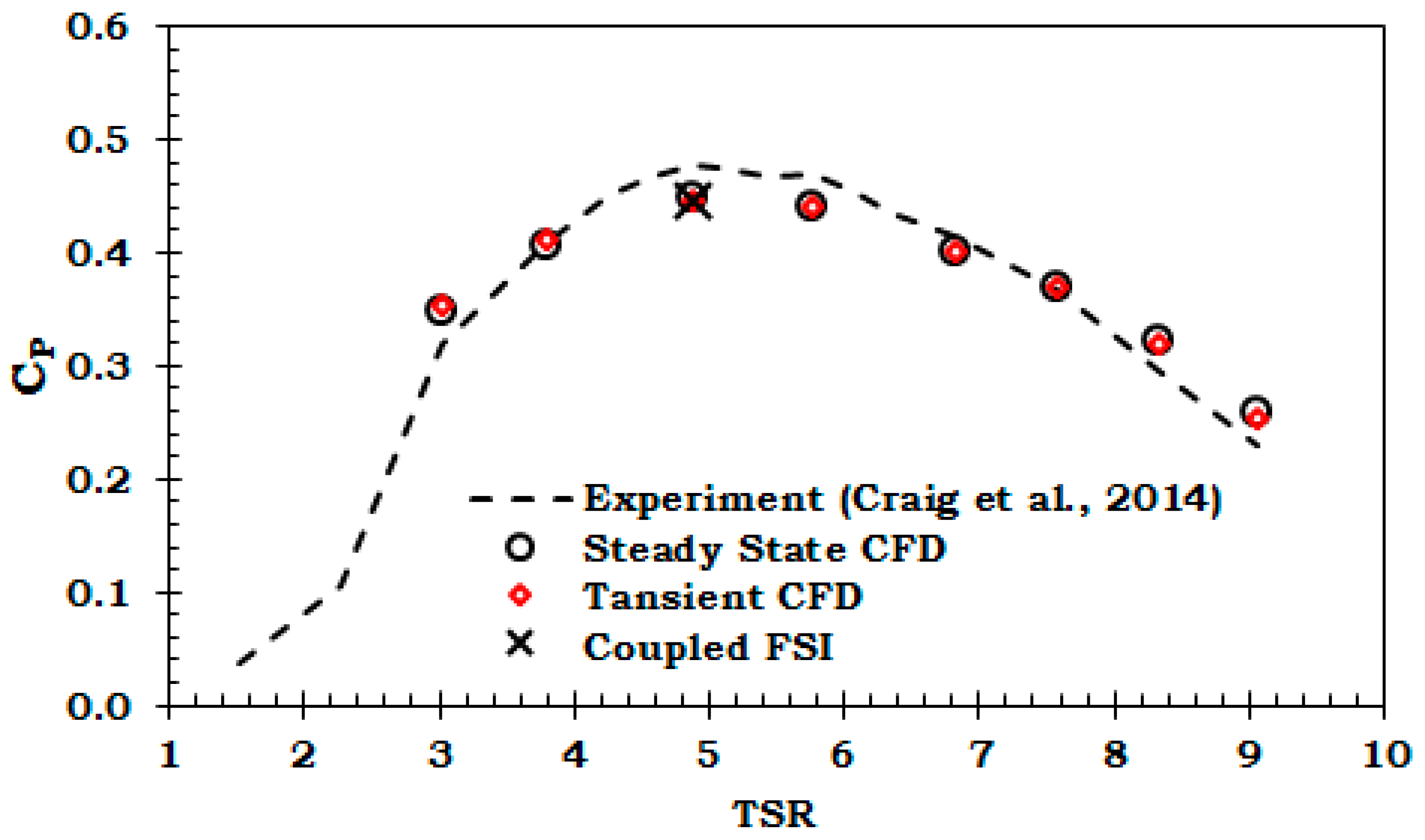
4. Verification and Validation of the Numerical Method

The accuracy of coupled FSI simulations depends largely on the constituent fluid and structural dynamic models. If the spatial and temporal discretization of the constituent fluid and structural dynamic models are verified then the other parameter that can possibly affect the accuracy of the coupled simulation is the mapping error in data transfer. In this paper, a mesh sensitivity is performed to verify that the fluid dynamic model is providing a mesh independent solution. For this purpose, the steady state CFD (MFR) model is utilized on four different grids generated with almost a similar mesh scheme but having different grid densities in the rotating and stationary domains (Table 2).
The meshing strategy is to use 70% or more elements in the rotating domain and keep the number of inflation layers and y + value nearly constant for all the grids utilized in the mesh sensitivity study. The MFR model is selected to eliminate the uncertainties associated with temporal discretization at this stage. The simulations are conducted at uniform velocity of 1.5 m/s and turbulence intensity of 5% with a viscosity ratio of 10 for the turbine operating at optimum TSR of 4.87. The value of torque on a single blade is a direct output of the CFD simulation and is used to evaluate the effect of grid density on the simulation results. Figure 4 shows that increasing the grid density monotonically increases the predicted torque value. The difference in the predicted values of torque for a single blade is only about 0.5% between the last two grids (Table 2). Therefore, the grid with 4.5 × 10⁶ elements (Grid 3) is selected for further simulations. To establish the temporal accuracy of the fluid dynamic model a time step sensitivity study is performed by utilizing the transient CFD model described in Section 3.1 with selected Grid 3. Three simulations at time steps corresponding to 2°, 4° and 6° of turbine rotations and total time corresponding to three turbine rotations are conducted at the optimum TSR 4.87 and each simulation is initialized by the steady flow solution. The difference between the torque values with respect to the 2° case is 0.08% and 0.32% for the 4° and 6° case respectively. The value of predicted torque is found to be less sensitive to the size of the time step. This observation is similar to the findings in other similar studies [47,49] and supported by the fact that ANSYS CFX is an implicit solver and does not require very small Courant numbers for stability [42]. Thus, a time step corresponding to 6° of turbine rotation is selected to ensure computational efficiency is achieved without compromising the accuracy and stability of the numerical solution.
To further validate the utilized numerical methods, power coefficients predicted by the steady state, transient analysis and coupled FSI analysis of the full-scale model are compared with model scale experimental data [39] in Figure 5 and Table 3.
All the numerical models predicted similar values to those measured in the experiment for the turbine power coefficient ( C p ) at the optimum TSR. Experimental values for turbine thrust coefficient (CT) are not available. However, all the numerical models predicted similar values of thrust coefficient ( C T ) . The turbine diameter-based Reynold number ( R e D = U × D / ν ) for the utilized turbine design in this study is 3 × 10⁷, whereas the turbine in the experiment has a Reynold number of 5.2 × 10⁵. But still the performance coefficients of full-scale model matched well with the scaled model experimental data. This observation is consistent with the findings in Reference [9] and supports the fact that performance in terms of non-dimensional parameters is independent of Reynold number beyond a critical value. To ensure the proper execution of data transfer between the fluid and structural dynamic models, the expert parameter “DumpInterfaceMeshes” in the FSI model setup is set to the CFD post. A summary of the data transfer report displayed on the solver run window of the coupled simulation and contour plot of “DumpInterfaceMeshes” showed that 100% of node data were successfully transmitted between the solvers.

5. Results and Discussion

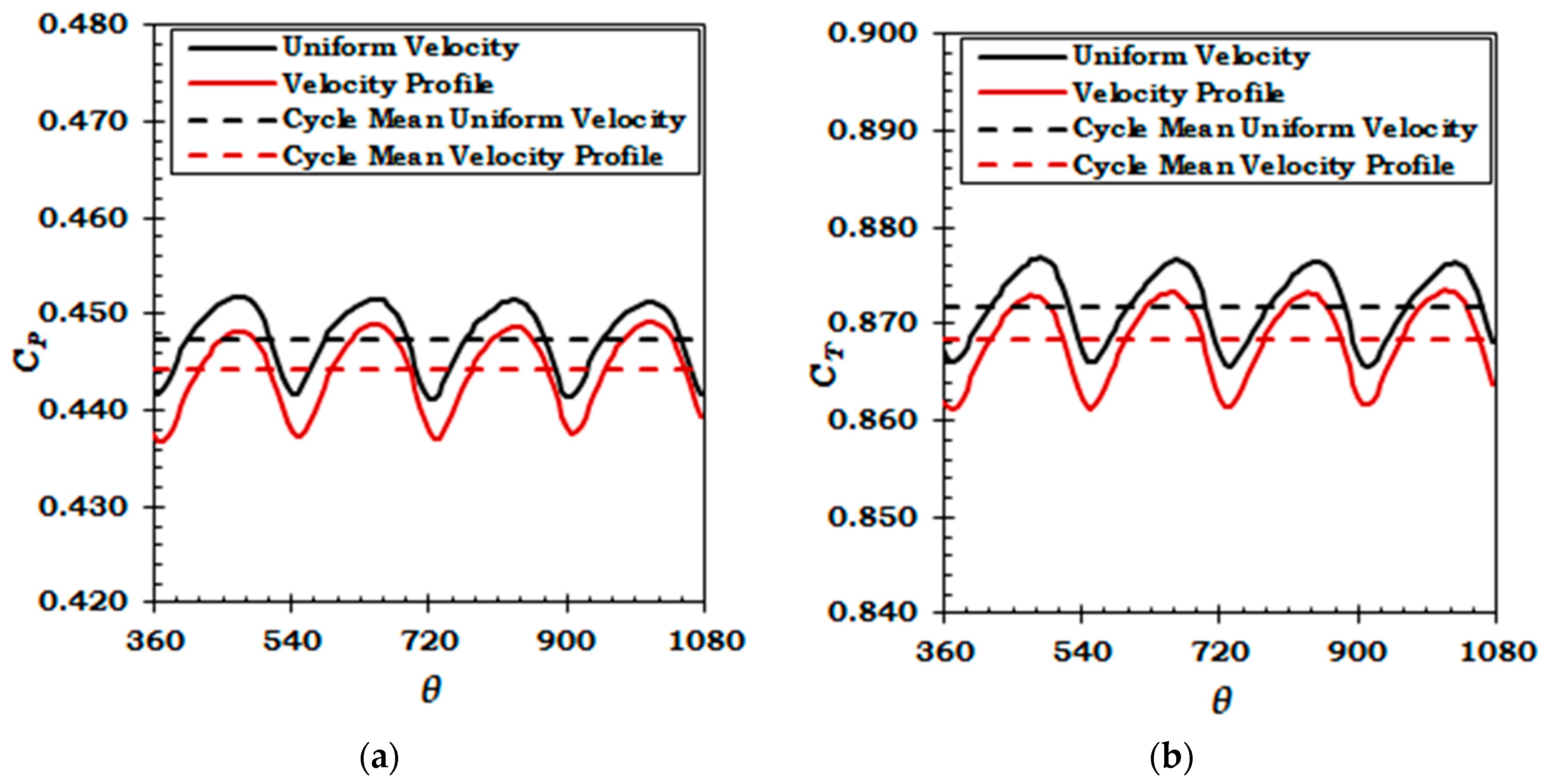
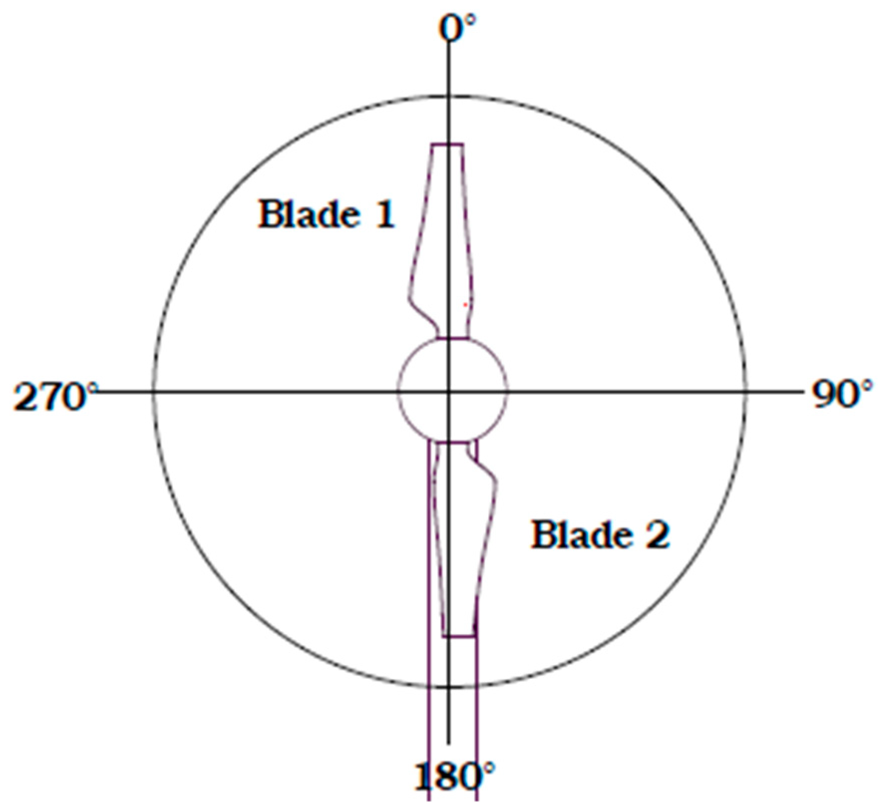
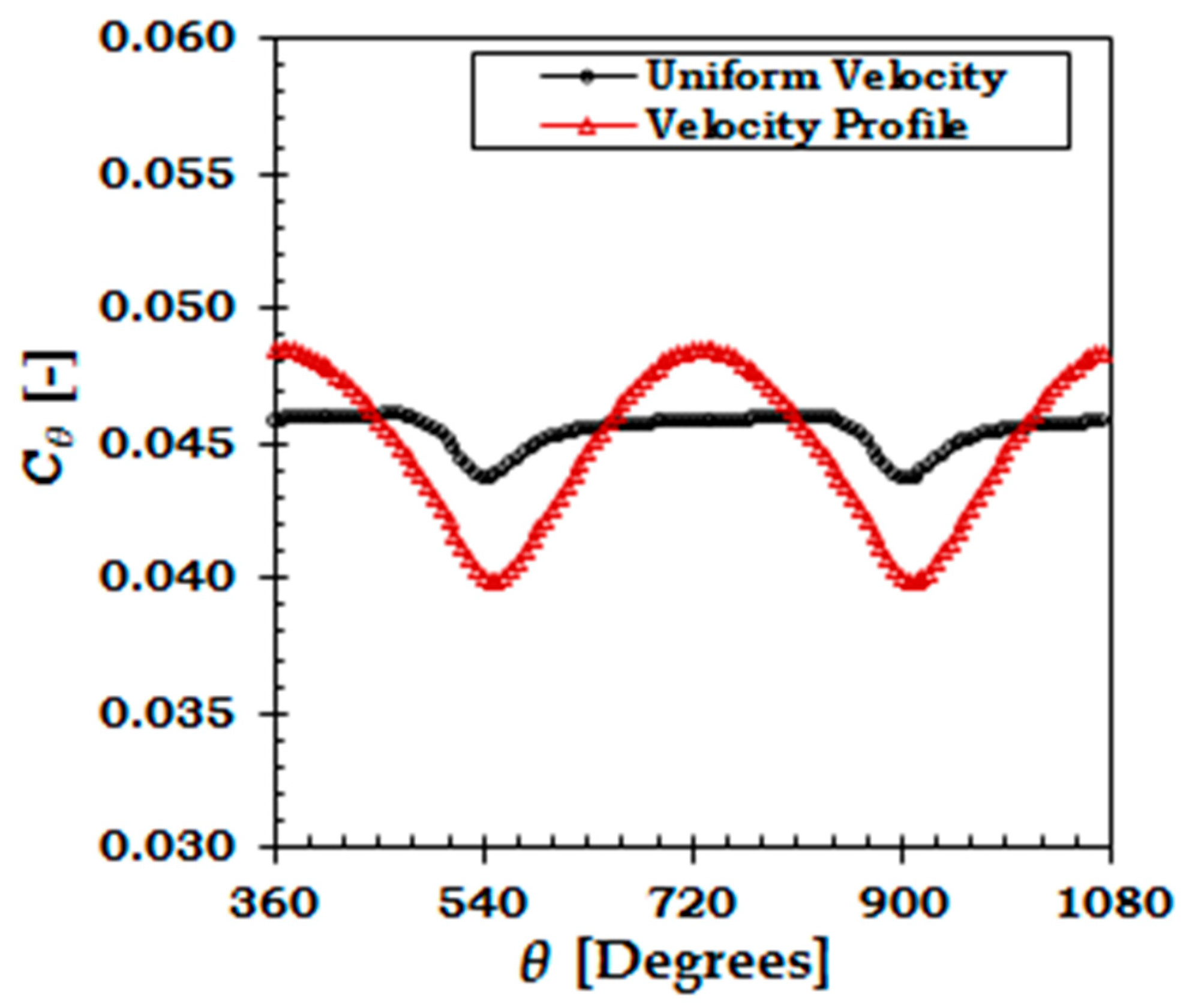
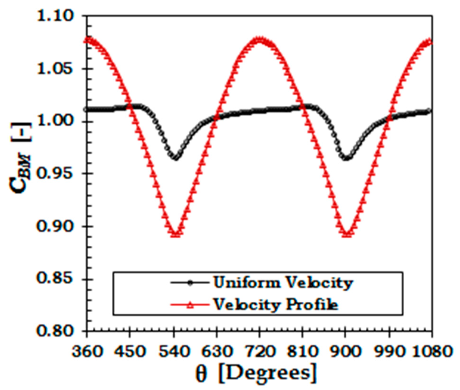
5.1. Effect of Velocity Profile on Variation of Structural Loads

Performance coefficients of the whole rotor, obtained from the FSI simulations, for a uniform inlet velocity and velocity profile are presented in Figure 6.
The mean cycle values of power and thrust coefficient have decreased by about 0.69% and 0.38%, respectively, due to the effect of velocity profile. The percentage drop in power and thrust coefficient is considerably small compared to Mason-Jones et al. [14]. This is mainly because of the velocity profile employed in this study. Two maxima and minima per cycle are evident in Figure 6, which are due to the effect of two blades passing the tower. When any of the turbine blade passes the tower, the whole rotor power and thrust drops below its mean value due to the tower effect. The whole rotor power and thrust coefficients vary from its mean value by 2.31% and 1.25% respectively due to the sole effect of tower. For a combined effect of velocity profile and tower the variation in power and thrust coefficients is 2.73% and 1.42% respectively. Although, it seems that velocity profile will complement the tower shadow effect in reducing the rotor power and thrust. Because when a blade passes the tower it is also operating in the lower part of the water column. However, Figure 6 shows that the combined effect of velocity profile and tower on the whole rotor power and thrust is not much different than the sole effect of tower. This finding is in accordance to similar studies for wind turbines [50,51]. This is because the rotor achieves its peak value near the horizontal position ( θ = 90 ° 270 ° ) (Figure 7). At this position, the effect of velocity profile is not prominent and the onset velocity is almost equal to the hub height velocity of the uniform velocity case. Therefore, the effect of velocity profile is almost negligible. Similarly, the rotor achieves minimum power when it is aligned vertically with the tower ( θ = 0 ° 180 ° ). At this position the lower blade experiences the maximum effect from tower and velocity profile. However, at the same time the upper blade is almost free from the effect of tower and operates in the maximum velocity region in the water column. Therefore, the cumulative effect balances out and the resultant combined effect of tower and velocity profile on the whole rotor power coefficient is not much extravagant. Contrarily, in the case of a single blade, the extreme values of the blade wise torque coefficient C θ (Figure 8) occur when a blade is aligned to the tower either at θ = 0 ° or θ = 180 ° .
The variation in mean cycle values of the thrust coefficient for the whole rotor is smaller than the power coefficient (Table 4). This observation is significant for the useful life of turbine shaft, bearings, seals and other associated components. It was anticipated that a two-bladed rotor would exhibit larger power and thrust coefficient variation compared to a tri-bladed rotor due to the effect of velocity profile and support tower. However, for a tri-bladed device [31] the mean cycle values of power coefficient varied by about 10% with three maxima and minima per cycle. The two-bladed device in this study and another similar study [16] showed a much lower variation in power coefficient of 2.73% and 5.72%, respectively, with two maxima and minima per cycle. However, since these studies utilized different turbine design and tidal conditions therefore, this conflict may be resolved by utilizing similar turbine design with different number of blades operating in similar flow conditions.
Flap wise bending moment at the blade root is considered a critical design load for causing blade failures [32]. Flap wise bending moment is caused by the moment of thrust force and acts along the chord line. The peak rotor loads predominantly come from the thrust characteristics of turbine. The thrust behavior of a single blade is similar to the flap wise blade bending moment but has not been shown here for brevity. Contrary to the total rotor loads, the velocity profile has a significant effect on the variation of individual blade loads (Figure 9).
Detailed quantitative evaluation of load variation on a single blade and whole rotor is provided in Table 4. This table clearly shows that the sole effect of tower on load variation on an individual blade is about twice the load variation on whole rotor. Due to the combined effect of velocity profile and tower, the variation in thrust coefficient from the mean cycle value of an individual blade increases from 2.8% to 9%. Whereas, for flap wise bending moment the addition of velocity profile increases the load variation on a single blade from 4.9% to 19%. The change in both these loads variation is quite significant and indicative of the importance of considering the velocity profile as a possible source of fatigue failure. For the uniform velocity case, the rotor thrust reduced by about 1.3% due to the tower shadow effect. A similar reduction in thrust of 1–2% due to tower shadow has been reported for wind turbines [50,51]. The mean value of the blade wise thrust decreases due to the combined effect of tower and velocity profile compared to the tower only effect (Table 4). But the peak and range of blade wise thrust increases resulting in increasing the variation. The thrust behavior between the two cases is significantly different from each other and can have serious consequences for the fatigue life of turbine components. For the sole effect of tower, both the blade will almost contribute a similar value of thrust that will be transferred to the shaft and associated components. The thrust force can be expected to act almost along the center line of the shaft. For the combined effect of tower and velocity profile the upper blade will contribute significantly more to the rotor thrust compared to the lower blade. The thrust force in this case will not act in axisymmetric manner and will affect the life of shaft, bearings, seals and other associated components. Moreover, the significant variation in flap wise bending moment reasserts its position as the most dominant and critical design load consideration for tidal turbine blade. Torque as a moment (edge-wise bending moment) and torsional bending moment are less critical and their contribution towards causing blade failure is not significant. Therefore, they are not discussed here in details. The torque variation is more relevant for the representation of power fluctuations and has been represented in terms of power coefficient variations in the earlier part of this discussion. The results presented so far in this paper are purely based on simulations and are not compared with full-scale experimental data due to the unavailability of required details. Nevertheless, this study is important as a preliminary step upon which future studies can be based. Additionally, we have selected the peak power operating condition because the largest bending moments will occur at this TSR [32].
Apart from load variations, the constituent fluid dynamic component of the coupled FSI analysis is capable to provide a very good visualization of the turbine flow field. Figure 10 shows that for uniform velocity case the wake is axisymmetric. The addition of velocity profile has shifted the wake upwards and velocity in the lower part of the wake has decreased. To further quantify this effect, velocity variation along the depth of the channel at different downstream locations is provided in Figure 11. The inflow velocity is unaffected up to a distance of 2D upstream (x/D = −2) in both cases. At the turbine location (x/D = 0) and 1D downstream (x/D = 1), the velocity variation is almost similar between the two cases. However, further downstream at (x/D = 3) and beyond that the wake has clearly shifted upwards. For the velocity profile case, the velocity in the upper bypass region of the wake has increased.
Figure 12 shows that for the uniform velocity case at 1D above and below the turbine, the velocity deficit gradually reduces along the channel length with almost a similar velocity recovery. However, for the velocity profile, at 1D above turbine the velocity deficit is negative throughout the length of the channel. This indicates that higher velocity than the mean free stream velocity is available at this height. This finding can be utilized for the future array designs as the power out of turbine is a function of the cube of velocity. In an axial array layout, if the downstream devices are positioned successively higher than the upstream devices, this higher velocity can be utilized to obtain higher power outputs. However, there are several other complications and site constraints that need to be further analyzed.

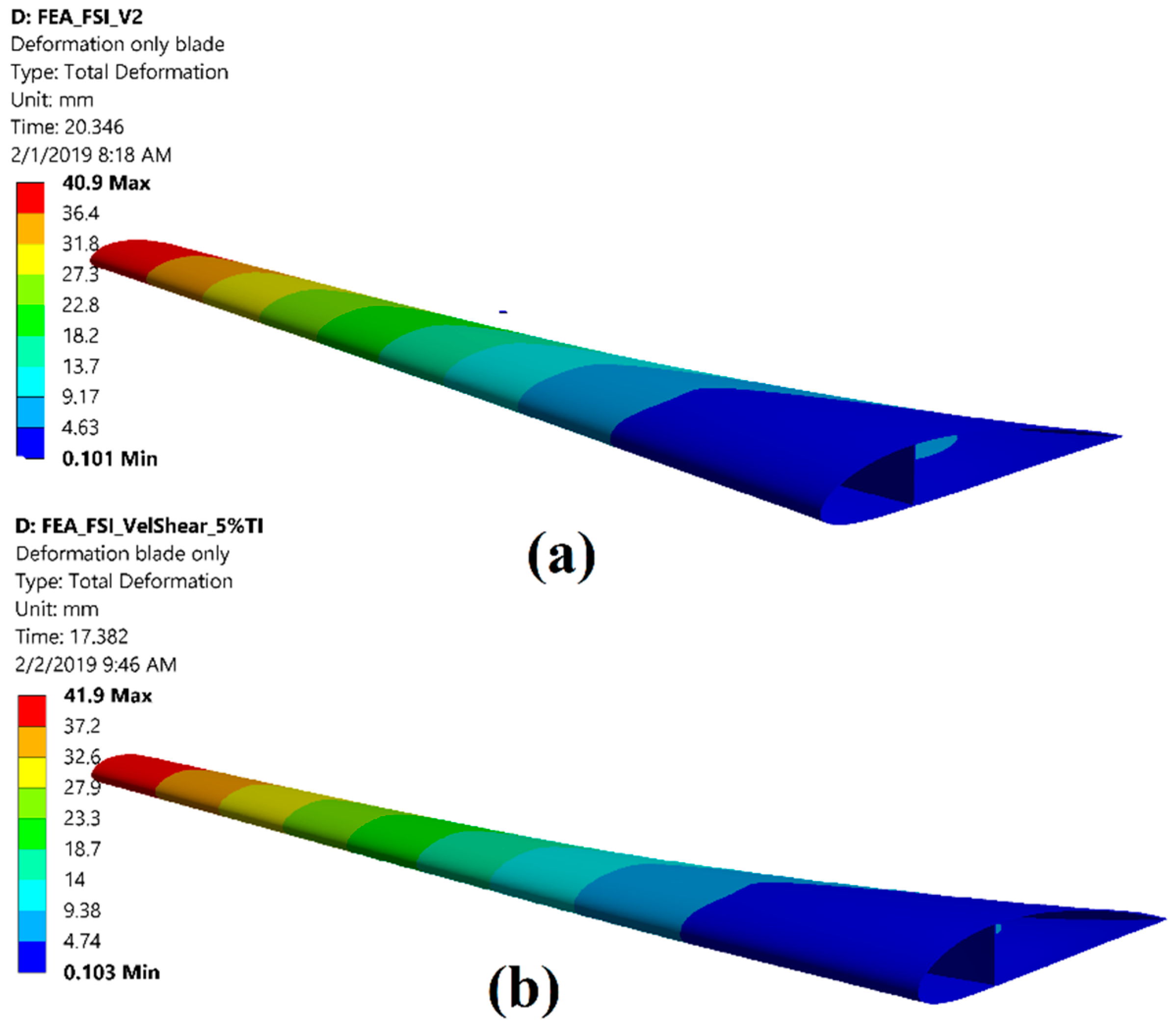
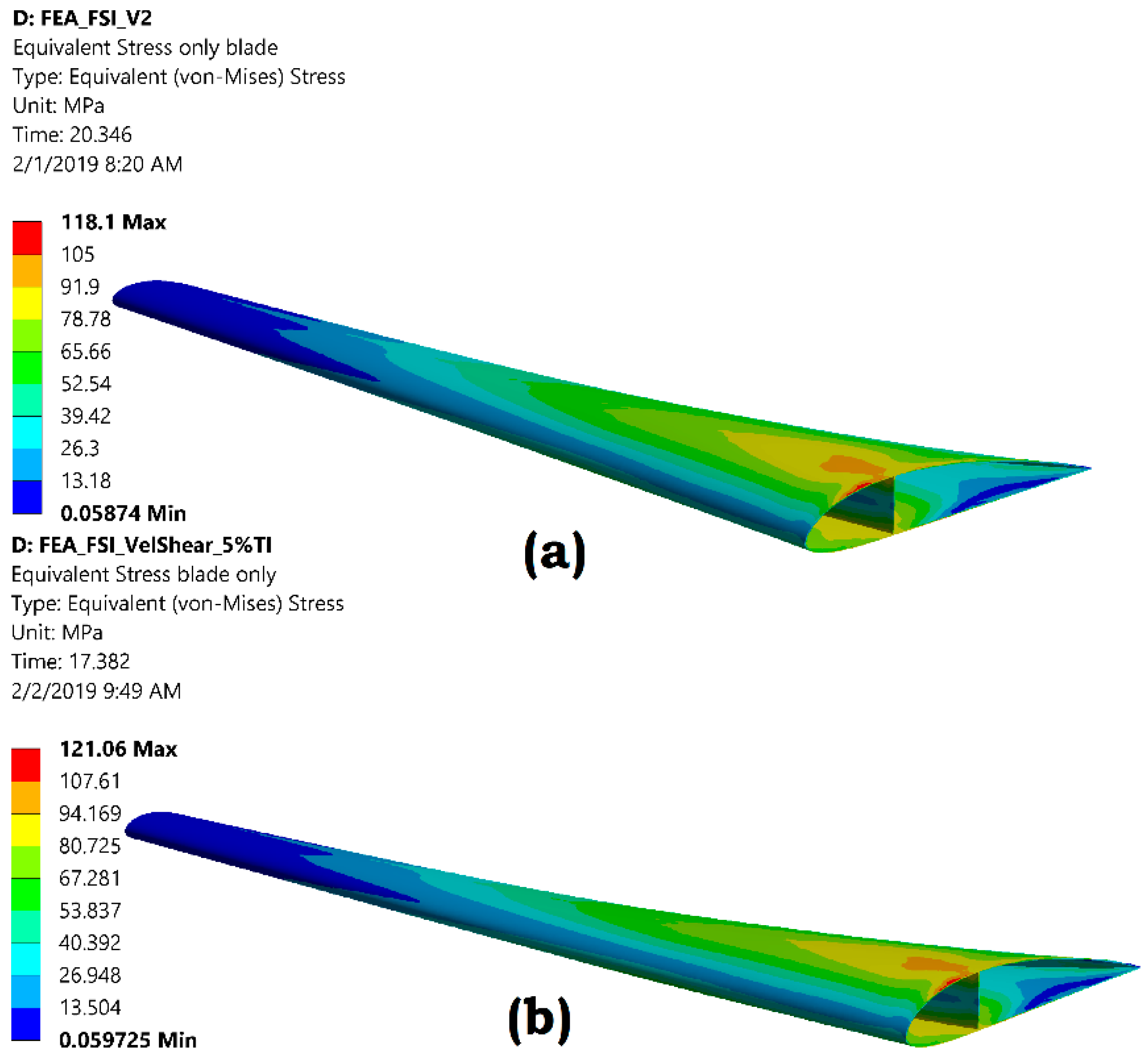
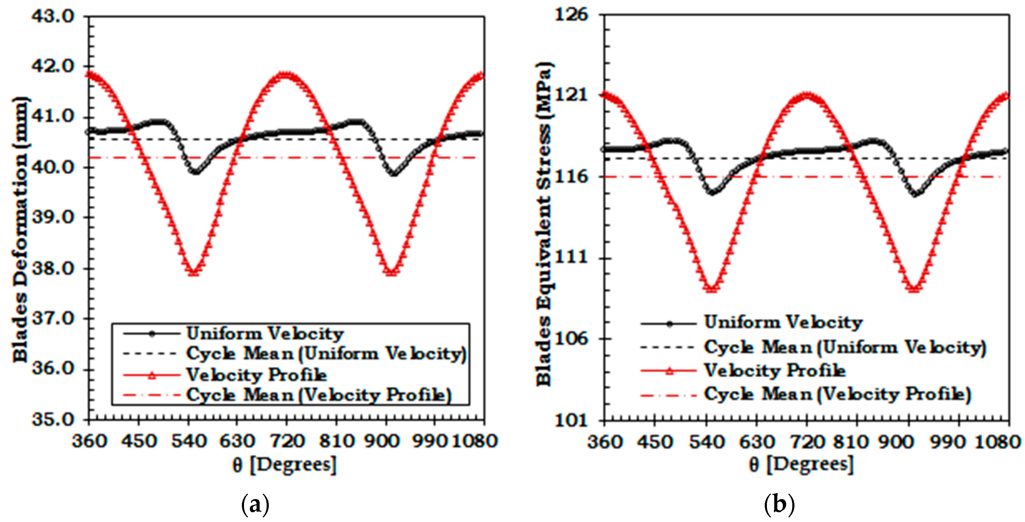
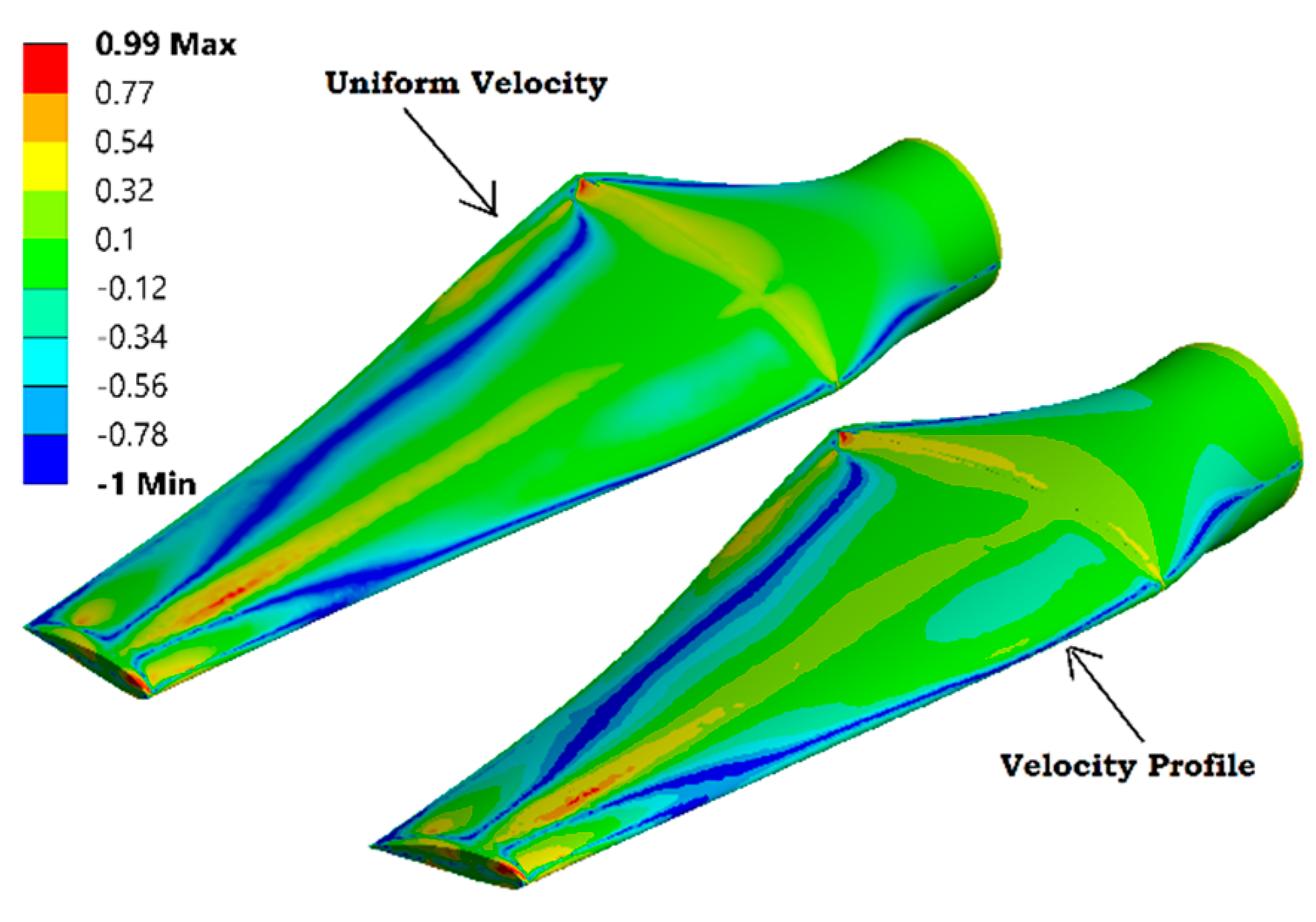
5.2. Effect of Velocity Profile on Variation of Stresses and Implications to Fatigue Life

The coupled FSI model provides a detailed insight into the structural response of turbine components against the imposed fluid loads by providing all the results that are possible from a standalone FEA analysis. The maximum blade deformation in the evaluated cases is relatively small about 40.9 mm for the uniform velocity case and 41.9 mm for the velocity profile (Figure 13). The maximum equivalent stress for the uniform velocity and velocity profile is 118 MPa and 121 MPa respectively (Figure 14). The maximum stress occurs near the root of the blade and it is clearly evident that this area would require additional reinforcement.
Figure 15 clearly shows that blade deformation and stress vary with the blade angular position during a rotation cycle. The blade deformation and stress vary by about 2.5% and 2.8%, respectively, from its mean cycle value during a rotation cycle due to the sole effect of the tower. The variation in blade deformation and equivalent stress are significantly increased to 9.8% and 10.3%, respectively, due to the added effect of velocity profile. The velocity profile augments the tower effect resulting in increased variation in blade deformation and stress. It is however interesting to note that the mean cycle value of deformation and stress decreases with the added effect of velocity profile (Table 5). Because, when a blade comes in front of the tower along its rotation cycle, at this moment it is in the lower velocity region of the water column. Therefore, the minimum value of thrust force is further reduced due to the combined effect of tower and velocity profile. Contrarily, when a blade is at the top, it is free from the tower effects and operates in the higher velocity region of the water column. Therefore, the maximum value of thrust force further increases due to the combined effect of tower and velocity profile. This reduction in the minimum value of thrust and increase in the maximum value of thrust causes a reduction in the mean value of stress due to the added effect of velocity profile. On the contrary, the values of range and variation are considerably increased. The mean stress and stress range (alternating stress) are the two important parameters with prominent effects on the fatigue life of turbine blade. The fatigue strength of the blade will decrease with increase in the mean stress and or stress range and vice versa. The fatigue strength under an axial load is decreased due to increase in the tensile mean stress. However, in case of torsion, the fatigue strength is unaffected by the increase or decrease in mean stress. For the case study presented in this paper, the mean stress decreases by a very little margin however, the stress range (alternating stress) increases considerably by more than three times due to the added effect of velocity profile. The stress response of the blade (Figure 15) shows a repeating cyclic behavior indicating the possibility of fatigue failure.
To further investigate the fatigue behavior of the rotating turbine blade, fatigue analysis was performed using a stress life fatigue model. The stress life fatigue model determines the total fatigue life and does not differentiate between crack initiation and propagation. The stress life fatigue model is based on S-N curve and deals with high cycle fatigue. A constant amplitude proportional loading was assumed because the principal stress axis does not change over time. A stress ratio, (R = σMin/σMax) of 0.97 and 0.90 is used for the uniform velocity and velocity profile case respectively. Fatigue S-N curves for materials are mostly generated from fully reversed constant amplitude experimental tests. For in service application such loading condition is very rare and mostly a mean stress will exist that must be accounted for in the fatigue analysis. In the stress life fatigue model of the ANSYS fatigue module the mean stress effect can be taken into account through direct interpolation between experimental S-N data. But such experimental data is usually not available due to the cost of experimental tests. Empirical relations like Goodman, Soderberg and Gerber theories can be used as an alternative to the experimental data. These empirical relations use the static material properties together with the S-N data to account for the mean stress effects. The experimental data generally lies between the Goodman and Gerber relation. For brittle materials, the Goodman relation is considered as a better choice whereas for the ductile materials the Gerber relation is often preferred. The turbine blades for the current study are made from structural steel and therefore a Gerber equation is selected. Equivalent (VonMises) stress was used as the stress component for the fatigue analysis to convert from a multiaxial stress state obtained from FE analysis to the uniaxial stress state of the experimental fatigue data.
Figure 16 shows the stress state of the blade for uniform velocity and velocity profile. The green color corresponds to a biaxiality indication of (0) indicating a uniaxial stress state at a majority of the blade. The blue color with a biaxiality indication of (−1) indicates a pure shear and red with a biaxiality indication of (1) represent a pure biaxial state. The contour plot clearly shows that the major portion of the blade is in a uniaxial stress state (green color) and S-N data for torsional loading is not required for the fatigue analysis of turbine blades. Figure 17 shows that for the uniform velocity the fatigue factor of safety is 3.8. The additional effect of velocity profile has reduced the fatigue factor of safety by about 8% to a value of 3.5. It is important to note that although this study utilized a near to real turbine design but only the hydrodynamic conditions of velocity profile is modeled with contribution to the fatigue failure of blades. But other important contributors, like turbulence and waves, etc., will also contribute to deciding the final fatigue life of the blade.

6. Conclusions and Prospects

3D Transient coupled FSI simulations have been performed using ANSYS Workbench 18.2 to quantify the effect of velocity profile on load variations for a large scale two-bladed complete tidal turbine. The utilized simulation method was validated with experimental data, and its spatial and temporal accuracy has been quantified. The turbine hydrodynamics and structural dynamics are simulated for two different inflow conditions, one representing a uniform inlet velocity and the other a velocity profile based on 1/7th power law. Results show that mean cycle values of both the power and thrust coefficient are 0.69% and 0.38% less for the velocity profile. In the case of uniform inlet velocity, the rotor power and thrust coefficients varied from their mean values by 2.31% and 1.25% respectively. This variation is caused by the turbine blades passing the support tower. For a combined effect of velocity profile and tower the variation in power and thrust coefficients increased to 2.73% and 1.42%, respectively. Therefore, the effect of velocity profile on the turbine power and thrust fluctuation is not significant for the evaluated turbine design and hydrodynamic conditions. Conversely, the velocity profile had a significant effect on the variation of individual blade loads. Due to the added effect of velocity profile, the variation in thrust coefficient of an individual blade increased from 2.8% to 9%. Additionally, for the flap-wise bending moment the velocity profile increased the variation on a single blade from 4.9% to 19%. The increase in loads variation is quite significant and indicative of the importance of considering the velocity profile as a possible source of fatigue failure. The thrust behavior between the two cases is significantly different from each other. For the sole effect of the tower, both blades contribute similar values of thrust that is transferred to the shaft and associated components. In this case, the thrust force is expected to act almost along the center line of the shaft. However, for the combined effect of tower and velocity profiles, the upper blade contributes significantly more to the rotor thrust than the lower blade. The thrust force, in this case, will not act in an axisymmetric manner and will affect the life of shaft, bearings, seals, and other associated components. Moreover, flap-wise bending moment has been found to have the highest variation, reasserting its position as the most dominant and critical design load consideration for turbine blade fatigue life. The blade deformation and stress varied by about 2.5% and 2.8%, respectively, from the mean cycle value during a rotation cycle due to the sole effect of the tower. The variation in blade deformation and equivalent stress are increased to a value of 9.8% and 10.3%, respectively, due to the added effect of the velocity profile. The stress response of blades showed a repeating cyclic behavior indicating the possibility of fatigue failure. The mean cycle value of deformation and stress decreases with the added effect of velocity profile. However, the range and variation are considerably increased. The added effect of velocity profile has reduced the fatigue factor of safety by 8% for the evaluated cases. An axisymmetric wake was observed for the uniform velocity case that was shifted upwards due to the effect of velocity profile. At 1D above the turbine, the velocity deficit is negative throughout the length of the channel in case of velocity profile. This indicates that higher velocity than the mean free stream velocity is available at this height. This finding can be utilized for future array designs as the power output of the turbine is a function of the cube of velocity. In an axial array layout, if the downstream devices are positioned successively higher than the upstream devices, this higher velocity can be utilized to obtain higher power outputs.
In this study, the effect of tower elasticity and wave action was not considered. In future studies, the addition of wave-current interaction with different velocity profiles and onset turbulence levels typically found in tidal flows may be considered. Future investigations may cover the entire range of TSR and should not be limited to the TSR of maximum blade load. Different fatigue models like strain life fatigue model and or a fracture mechanics-based fatigue model may be useful to uncover other aspects of the fatigue behavior of a tidal turbine blade.

Author Contributions

J.V., S.B. and M.B. conceptualized the research theme and planned this research study. M.B. and S.J. designed the research methodology and prepared the simulations. M.A. and S.A.M. made several revisions and suggested improvements to the final manuscript. M.B. performed all the simulations and post-processed, analyzed the results, and wrote the manuscript. All authors read and approved the final manuscript.

Funding

This research received no external funding and The APC are paid by the author.

Acknowledgments

The authors gratefully acknowledge the support of the Department of Aeronautics and Astronautics at the Institute of Space Technology Islamabad for providing computational facilities at the modeling and simulation laboratory. The Higher Education Commission (HEC) Pakistan is also acknowledged for its financial support to scholar Mujahid Badshah, Pin#2EG1-384.

Conflicts of Interest

The authors declare no conflict of interest.

References

  1. Milne, I.A.; Sharma, R.N.; Flay, R.G.; Bickerton, S. Characteristics of the turbulence in the flow at a tidal stream power site. Philos. Trans. R. Soc. A 2013, 371, 20120196. [Google Scholar] [CrossRef] [PubMed]
  2. Jones, J.; Davies, A. Influence of wave-current interaction, and high frequency forcing upon storm induced currents and elevations. Estuar. Coast. Shelf Sci. 2001, 53, 397–413. [Google Scholar] [CrossRef]
  3. Zeiner-Gundersen, D.H. Turbine design and field development concepts for tidal, ocean, and river applications. Energy Sci. Eng. 2015, 3, 27–42. [Google Scholar] [CrossRef]
  4. Maganga, F.; Germain, G.; King, J.; Pinon, G.; Rivoalen, E. Experimental characterisation of flow effects on marine current turbine behaviour and on its wake properties. IET Renew. Power Gen. 2010, 4, 498–509. [Google Scholar] [CrossRef] [Green Version]
  5. Barltrop, N.; Varyani, K.; Grant, A.; Clelland, D.; Pham, X. Investigation into wave—Current interactions in marine current turbines. Proc. Inst. Mech. Eng. Part A J. Power Energy 2007, 221, 233–242. [Google Scholar] [CrossRef]
  6. Luznik, L.; Flack, K.A.; Lust, E.E.; Taylor, K. The effect of surface waves on the performance characteristics of a model tidal turbine. Renew. Energy 2013, 58, 108–114. [Google Scholar] [CrossRef]
  7. Blackmore, T.; Myers, L.E.; Bahaj, A.S. Effects of turbulence on tidal turbines: Implications to performance, blade loads, and condition monitoring. Int. J. Mar. Energy 2016, 14, 1–26. [Google Scholar] [CrossRef] [Green Version]
  8. Mycek, P.; Gaurier, B.; Germain, G.; Pinon, G.; Rivoalen, E. Experimental study of the turbulence intensity effects on marine current turbines behaviour. Part I: One single turbine. Renew. Energy 2014, 66, 729–746. [Google Scholar] [CrossRef] [Green Version]
  9. Mason-Jones, A.; O’doherty, D.; Morris, C.; O’doherty, T.; Byrne, C.; Prickett, P.; Grosvenor, R.; Owen, I.; Tedds, S.; Poole, R. Non-dimensional scaling of tidal stream turbines. Energy 2012, 44, 820–829. [Google Scholar] [CrossRef]
  10. Draper, S.; Nishino, T.; Adcock, T.; Taylor, P. Performance of an ideal turbine in an inviscid shear flow. J. Fluid Mech. 2016, 796, 86–112. [Google Scholar] [CrossRef] [Green Version]
  11. Batten, W.; Bahaj, A.; Molland, A.; Chaplin, J. The prediction of the hydrodynamic performance of marine current turbines. Renew. Energy 2008, 33, 1085–1096. [Google Scholar] [CrossRef]
  12. Lewis, M.; Neill, S.; Robins, P.; Hashemi, M. Resource assessment for future generations of tidal-stream energy arrays. Energy 2015, 83, 403–415. [Google Scholar] [CrossRef] [Green Version]
  13. Blunden, L.; Bahaj, A. Tidal energy resource assessment for tidal stream generators. Proc. Inst. Mech. Eng. Part A J. Power Energy 2007, 221, 137–146. [Google Scholar] [CrossRef]
  14. Mason-Jones, A.; O’doherty, D.; Morris, C.; O’doherty, T. Influence of a velocity profile & support structure on tidal stream turbine performance. Renew. Energy 2013, 52, 23–30. [Google Scholar]
  15. Tatum, S.; Allmark, M.; Frost, C.; O’Doherty, D.; Mason-Jones, A.; O’Doherty, T. CFD modelling of a tidal stream turbine subjected to profiled flow and surface gravity waves. Int. J. Mar. Energy 2016, 15, 156–174. [Google Scholar] [CrossRef] [Green Version]
  16. Yahagi, K.; Takagi, K. Moment loads acting on a blade of an ocean current turbine in shear flow. Ocean Eng. 2019, 172, 446–455. [Google Scholar] [CrossRef]
  17. Muchala, S.; Willden, R.H. Influence of support structures on tidal turbine power output. J. Fluids Struct. 2018, 83, 27–39. [Google Scholar] [CrossRef]
  18. Li, H.; Hu, Z.; Chandrashekhara, K.; Du, X.; Mishra, R. Reliability-based fatigue life investigation for a medium-scale composite hydrokinetic turbine blade. Ocean Eng. 2014, 89, 230–242. [Google Scholar] [CrossRef]
  19. McCann, G. Tidal current turbine fatigue loading sensitivity to waves and turbulence—A parametric study. In Proceedings of the 7th European Wave and Tidal Energy Conference, Porto, Portugal, 11–13 September 2007. [Google Scholar]
  20. Bahaj, A.; Molland, A.; Chaplin, J.; Batten, W. Power and thrust measurements of marine current turbines under various hydrodynamic flow conditions in a cavitation tunnel and a towing tank. Renew. Energy 2007, 32, 407–426. [Google Scholar] [CrossRef]
  21. Stallard, T.J.; Feng, T.; Stansby, P.K. Experimental study of the mean wake of a tidal stream rotor in a shallow turbulent flow. J. Fluids Struct. 2015, 54, 235–246. [Google Scholar] [CrossRef]
  22. Draycott, S.; Payne, G.; Steynor, J.; Nambiar, A.; Sellar, B.; Venugopal, V. An experimental investigation into non-linear wave loading on horizontal axis tidal turbines. J. Fluids Struct. 2019, 84, 199–217. [Google Scholar] [CrossRef]
  23. Fernandez-Rodriguez, E.; Stallard, T.J.; Stansby, P.K. Experimental study of extreme thrust on a tidal stream rotor due to turbulent flow and with opposing waves. J. Fluids Struct. 2014, 51, 354–361. [Google Scholar] [CrossRef]
  24. Gaurier, B.; Davies, P.; Deuff, A.; Germain, G. Flume tank characterization of marine current turbine blade behaviour under current and wave loading. Renew. Energy 2013, 59, 1–12. [Google Scholar] [CrossRef] [Green Version]
  25. Milne, I.; Day, A.; Sharma, R.; Flay, R. Blade loading on tidal turbines for uniform unsteady flow. Renew. Energy 2015, 77, 338–350. [Google Scholar] [CrossRef]
  26. Milne, I.; Day, A.; Sharma, R.; Flay, R. The characterisation of the hydrodynamic loads on tidal turbines due to turbulence. Renew. Sustain. Energy Rev. 2016, 56, 851–864. [Google Scholar] [CrossRef]
  27. Payne, G.S.; Stallard, T.; Martinez, R.; Bruce, T. Variation of loads on a three-bladed horizontal axis tidal turbine with frequency and blade position. J. Fluids Struct. 2018, 83, 156–170. [Google Scholar] [CrossRef]
  28. Xia, Y.; Takagi, K. Effect of shear flow on a marine current turbine. In Proceedings of the Oceans, Shanghai, China, 10–13 April 2016; pp. 1–5. [Google Scholar]
  29. Kang, S.; Borazjani, I.; Colby, J.A.; Sotiropoulos, F. Numerical simulation of 3D flow past a real-life marine hydrokinetic turbine. Adv. Water Resour. 2012, 39, 33–43. [Google Scholar] [CrossRef]
  30. Tedds, S.; Owen, I.; Poole, R. Near-wake characteristics of a model horizontal axis tidal stream turbine. Renew. Energy 2014, 63, 222–235. [Google Scholar] [CrossRef] [Green Version]
  31. Ahmed, U.; Apsley, D.; Afgan, I.; Stallard, T.J.; Stansby, P.K. Fluctuating loads on a tidal turbine due to velocity shear and turbulence: Comparison of CFD with field data. Renew. Energy 2017, 112, 235–246. [Google Scholar] [CrossRef] [Green Version]
  32. Ouro, P.; Harrold, M.; Stoesser, T.; Bromley, P. Hydrodynamic loadings on a horizontal axis tidal turbine prototype. J. Fluids Struct. 2017, 71, 78–95. [Google Scholar] [CrossRef] [Green Version]
  33. Ouro, P.; Stoesser, T. Impact of Environmental Turbulence on the Performance and Loadings of a Tidal Stream Turbine. Flow Turbul. Combust. 2018, 102, 613–639. [Google Scholar] [CrossRef] [Green Version]
  34. Grogan, D.M.; Leen, S.B.; Kennedy, C.; Brádaigh, C.Ó. Design of composite tidal turbine blades. Renew. Energy 2013, 57, 151–162. [Google Scholar] [CrossRef] [Green Version]
  35. Suzuki, T.; Mahfuz, H. Analysis of large-scale ocean current turbine blades using Fluid–Structure Interaction and blade element momentum theory. Ships Off Shore Struct. 2018, 13, 451–458. [Google Scholar] [CrossRef]
  36. Nicholls-Lee, R.; Turnock, S.; Boyd, S. Application of bend-twist coupled blades for horizontal axis tidal turbines. Renew. Energy 2013, 50, 541–550. [Google Scholar] [CrossRef]
  37. Tatum, S.; Frost, C.; Allmark, M.; O’Doherty, D.; Mason-Jones, A.; Prickett, P.; Grosvenor, R.; Byrne, C.; O’Doherty, T. Wave-current interaction effects on tidal stream turbine performance and loading characteristics. Int. J. Mar. Energy 2016, 14, 161–179. [Google Scholar] [CrossRef]
  38. Badshah, M.; Badshah, S.; Kadir, K. Fluid Structure Interaction Modelling of Tidal Turbine Performance and Structural Loads in a Velocity Shear Environment. Energies 2018, 11, 1837. [Google Scholar] [CrossRef]
  39. Craig, H.; Vincent, S.N.; Budi, G.; Michele, G.; Fotis, S.U.S. Department of energy reference model program RM1: Experimental results. Dynamic Pose test, 2 December 2014. [Google Scholar]
  40. Hagerman, G.; Polagye, B. Methodology for estimating tidal current energy resources and power production by tidal in-stream energy conversion (TISEC) devices, EPRI North American Tidal In Stream Power Feasibility Demonstration Project. EPRI-TP-001 NA Rev 2. 2006. Available online: http://www.pstidalenergy.org/Tidal_Energy_Projects/Misc/EPRI_Reports_and_Presentations/EPRI-TP-001_Guidlines_Est_Power_Production_14Jun06.pdf (accessed on 11 June 2019).
  41. ANSYS Inc. ANSYS CFX-Solver Modelling Guide; ANSYS, Inc.: Southpointe 2600 ANSYS Drive Canonsburg, PA, USA, 2016. [Google Scholar]
  42. ANSYS Inc. ANSYS CFX-Solver Theory Guide; ANSYS, Inc.: Southpointe 2600 ANSYS Drive Canonsburg, PA, USA, 2016. [Google Scholar]
  43. Badshah, M.; VanZwieten, J.; Badshah, S.; Jan, S. CFD study of blockage ratio and boundary proximity effects on the performance of a tidal turbine. IET Renew. Power Gen. 2019. [Google Scholar] [CrossRef]
  44. Sufian, S.F.; Li, M.; O’Connor, B.A. 3D modelling of impacts from waves on tidal turbine wake characteristics and energy output. Renew. Energy 2017, 114, 308–322. [Google Scholar] [CrossRef] [Green Version]
  45. Tian, W.; VanZwieten, J.H.; Pyakurel, P.; Li, Y. Influences of yaw angle and turbulence intensity on the performance of a 20 kW in-stream hydrokinetic turbine. Energy 2016, 111, 104–116. [Google Scholar] [CrossRef] [Green Version]
  46. O’Doherty, T.; Mason-Jones, A.; O’Doherty, D.; Byrne, C.; Owen, I.; Wang, Y. Experimental and computational analysis of a model horizontal axis tidal turbine. In Proceedings of the 8th European Wave and Tidal Energy Conference (EWTEC), Uppsala, Sweden, 7–10 September 2009. [Google Scholar]
  47. Nitin, K.; Arindam, B. Performance characterization and placement of a marine hydrokinetic turbine in a tidal channel under boundary proximity and blockage effects. Appl. Energy 2015, 148, 121–133. [Google Scholar] [CrossRef]
  48. Davide, M.; Andreas, U. 2014 JRC Ocean Energy Status Report; Publications Office of the European Union: Luxembourg, Luxembourg, 2015; Available online: https://setis.ec.europa.eu/sites/default/files/reports/2014-JRC-Ocean-Energy-Status-Report.pdf (accessed on 11 June 2019).
  49. Lawson, M.J.; Li, Y.; Sale, D.C. Development and verification of a computational fluid dynamics model of a horizontal-axis tidal current turbine. In Proceedings of the ASME 2011 30th International Conference on Ocean, Offshore and Arctic Engineering, Rotterdam, The Netherlands, 19–24 June 2011; American Society of Mechanical Engineers: Rotterdam, The Netherlands, 2011; pp. 711–720. [Google Scholar]
  50. Zahle, F.; Sørensen, N. Overset grid flow simulation on a modern wind turbine. In Proceedings of the 26th AIAA Applied Aerodynamics Conference, Honolulu, HI, USA, 18–21 August 2008; p. 6727. [Google Scholar]
  51. Zahle, F.; Sørensen, N.N.; Johansen, J. Wind turbine rotor-tower interaction using an incompressible overset grid method. Wind Energy 2009, 12, 594–619. [Google Scholar] [CrossRef]
Figure 1. Velocity profile based on 1/7th power law (dashed lines represent turbine location).
Energies 12 02217 g001
Figure 2. Dimensions of the (a) Fluid domain; (b) Turbine.
Energies 12 02217 g002
Figure 3. Mesh used for the simulations (a) CFD Mesh; (b) FEA Mesh.
Energies 12 02217 g003
Figure 4. Variation of blade torque with grid density.
Energies 12 02217 g004
Figure 5. Comparison of experimental and simulated performance curves.
Energies 12 02217 g005
Figure 6. Rotor (a) power coefficient; (b) thrust coefficient.
Energies 12 02217 g006
Figure 7. Rotor angular positions for the presentation of results.
Energies 12 02217 g007
Figure 8. Variation of torque coefficient Cθ for Blade 1 during two rotation cycles.
Energies 12 02217 g008
Figure 9. Flap-wise bending moment (normalized by cycle mean) for Blade 1 during two rotations.
Energies 12 02217 g009
Figure 10. Axial velocity (normalized by the free stream velocity) contour for (a) uniform inlet velocity; (b) velocity profile.
Energies 12 02217 g010
Figure 11. Velocity variation along depth of the channel at different downstream location for (a) uniform velocity; (b) velocity profile (the red dash dotted line represent location of turbine hub center and the black dashed lines represent the extent of blade tips).
Energies 12 02217 g011
Figure 12. Velocity deficit along the length of the channel at different channel depths for (a) uniform velocity; (b) velocity profile.
Energies 12 02217 g012
Figure 13. Contour plot of blade deformation for (a) uniform velocity; (b) velocity profile.
Energies 12 02217 g013
Figure 14. Contour plot of blade equivalent stress for (a) uniform velocity; (b) velocity profile.
Energies 12 02217 g014
Figure 15. Variation of Blade 1 (a) deformation; (b) equivalent stress during two rotation cycles.
Energies 12 02217 g015
Figure 16. Biaxiality indication for the blade in uniform velocity and velocity profiles.
Energies 12 02217 g016
Figure 17. Fatigue factor of safety for blade (a) uniform velocity; (b) Velocity profile.
Energies 12 02217 g017
Table 1. Properties of the utilized structural steel material.
Density7850Kg/m3
Young Modulus2 × 1011Pa
Poisson’s Ratio0.3(-)
Tensile Yield Strength2.5 × 108Pa
Compressive Yield Strength2.5 × 108Pa
Tensile Ultimate Strength4.60 × 108Pa
Table 2. Mesh details for sensitivity analysis.
GridNo. of Elements (× 106)Torque Difference 1
Inner DomainOuter DomainTotal(%)
11.340.722.07−3.2
22.231.073.30−1.1
33.101.404.50−0.5
45.022.397.42-
1 % Torque difference denotes the difference of predicted torque value from each grid with respect to Grid 4.
Table 3. Quantitative comparison of turbine CP between simulations and experiment.
TSRExperimentSteady State CFDTransient CFDCoupled FSI
CP [39]CP% Difference 1CP% Difference 1CP% Difference 1
3.020.3200.3478.50.35410.7--
3.790.4080.4060.40.4110.8--
4.870.4770.4495.80.4476.30.4476.2
5.760.4710.4406.60.4426.2--
6.820.4140.4013.20.4022.8--
7.570.3680.3690.40.3680.1--
8.320.2950.3229.20.3198.2--
9.050.2300.26013.00.25410.4--
1 % Difference indicates the absolute percentage difference to the experimental value in Reference [39].
Table 4. Turbine loads variation during a rotation cycle.
ParameterValueUniform VelocityVelocity Shear
Single BladeRotorSingle BladeRotor
Thrust CoefficientPeak0.4370.8770.4450.869
Mean0.4330.8720.4290.864
Range0.0120.0110.0390.012
% Variation 12.81.39.01.4
Torque CoefficientPeak0.0460.0930.0480.092
Mean0.0450.0920.0450.091
Range0.0020.0020.0090.002
% Variation 15.22.319.32.7
Flap Wise Bending Moment CoefficientPeak1.013-1.078-
Mean1.0-1.0-
Range0.049-0.185-
% Variation 14.9-18.5-
1 % Variation indicates the variation from mean cycle value during a rotation.
Table 5. Turbine load fluctuations from the last rotation cycle.
ParameterValueUniform VelocityVelocity Profile
Deformation [mm]Peak40.941.9
Mean40.640.2
Range1.03.9
% Variation 1 2.59.8
Stress [MPa]Peak118.1121.1
Mean117.1116.0
Range3.212.0
% Variation 1 2.810.3
1 % Variation denotes variation from cycle mean value during a rotation cycle.

