Article

Reducing Computational Load for Mixed Integer Linear Programming: An Example for a District and an Island Energy System

1
Institute of Energy and Climate Research, Electrochemical Process Engineering (IEK-3), Forschungszentrum Jülich, D-52425 Jülich, Germany
2
Chair for Fuel Cells, RWTH Aachen University, c/o Institute of Electrochemical Process Engineering (IEK-3), Forschungszentrum Jülich GmbH, Wilhelm-Johnen-Str., 52428 Jülich, Germany
3
Westnetz GmbH, Florianstraße 15-21, 44139 Dortmund, Germany
4
Innogy SE, Kruppstraße 5, 45128 Essen, Germany
*
Author to whom correspondence should be addressed.
Submission received: 2 July 2019 / Revised: 18 July 2019 / Accepted: 19 July 2019 / Published: 22 July 2019

Abstract

:
The complexity of Mixed-Integer Linear Programs (MILPs) increases with the number of nodes in energy system models. An increasing complexity constitutes a high computational load that can limit the scale of the energy system model. Hence, methods are sought to reduce this complexity. In this paper, we present a new 2-Level Approach to MILP energy system models that determines the system design through a combination of continuous and discrete decisions. On the first level, data reduction methods are used to determine the discrete design decisions in a simplified solution space. Those decisions are then fixed, and on the second level the full dataset is used to ex-tract the exact scaling of the chosen technologies. The performance of the new 2-Level Approach is evaluated for a case study of an urban energy system with six buildings and an island system based on a high share of renewable energy technologies. The results of the studies show a high accuracy with respect to the total annual costs, chosen system structure, installed capacities and peak load with the 2-Level Approach compared to the results of a single level optimization. The computational load is thereby reduced by more than one order of magnitude.

1. Introduction

Urban districts are in search of strategies to reduce greenhouse gas (GHG) emissions. The strategies should be cost- and environmentally optimal solutions for future district energy supply systems. Microgrids have the potential to contribute to GHG reductions in urban districts because of their higher efficiency due to energy utilization synergies [1].
In the literature, microgrids are usually divided into microgrids with grid connection to the macrogrid and island microgrids without a connection to a higher grid level [2,3,4]. A microgrid can include multiple residential and commercial buildings with specific electricity, heating and cooling demands. These are supplied by conventional technologies like boilers, distributed energy resources (DERs) such as photovoltaics (PV), energy storages technologies like batteries, and different energy distribution grids for electricity, natural gas and district heating [5,6,7]. The advantage of microgrids is the cost-optimal operation of supply technologies through exchanging the energy between the buildings and storing it [8].

1.1. The Complexity of Microgrid Supply System Optimization

Determining the optimal design and operation of microgrids is a complex task that imposes demanding requirements on computational resources and mathematical solvers. Different mathematical approaches, such as Mixed-Integer Linear Programming (MILP) [2,4,6,9,10,11,12,13], Mixed-Integer Non-Linear Programming (MINLP) [14,15] and metaheuristic approaches [3,16,17] are used to determine the optimal design or operation of microgrid energy supply systems. The advantage of mathematical programming like MILP to metaheuristics is that the distance to the global optimum can be determined, which increases the quality of the results. On the other hand, the computing time is high with MILP, as shown in Morvaj et al. [10] and, especially for Mixed Integer Non-Linear Programming [15] metaheuristic approaches, allows for a higher spatial resolution compared to mathematical programming because of lower complexity, but the global optimum is not guaranteed.
Mehleri et al. [6] developed a MILP model to design and operate a cost-optimal energy supply system for a five-building neighbourhood in Greece. The conceptualized microgrid contains a boiler, a combined heat and power plant (CHP), PV and thermal storage capacity, along with an electrical and natural gas macrogrid connection, as well as a local district heating network. A metaheuristic approach was developed by Prousch et al. [17] to schedule the operation of heat pumps, CHP units and electric vehicles in a district with 69 nodes, which includes 10,074 households with commercial and residential buildings. Olivares et al. [15] present a MINLP approach for the operation of microgrids. A non-linear approach was used to manage the reactive power in the distribution grid, such that the model complexity was higher than in a linear mathematical program, as in a MILP model.
Furthermore, Morvaj et al. [9] present a multi-objective MILP approach to optimize the economic, environmental and technical criteria and compare it with a bi-level as well as a combined approach of MILP and bi-level optimization. The optimal design and operation were focused on five residential buildings by adding grid constraints. These constraints are used in terms of linearized AC power flow for the MILP and nonlinear AC power flow for the bi-level approach. In the combined approach, linear and nonlinear AC power flow is used in order to check the accuracy of the linearized results. In comparison to the MILP approach, the bi-level approach shows better solving performance, while the optimality is not guaranteed. The combined approach has the best overall performance for optimality, accuracy and solving performance. Another MILP model was developed by Omu et al. [11] and applied in a case study in Southern England in a six-building case study to investigate an electrification and standalone CHP scenario with different degrees of decentralization.

1.2. State of the Art of Complexity Reduction

Systematic reduction of model complexity is often used to solve design and operation optimization problems on different energy system levels, e.g., reducing the complexity through decomposition, as in Falke et al. [16], to determine the cost- and environmentally optimal technology configuration of a microgrid on the basis of a metaheuristic approach. The optimization problem was decomposed into three subproblems to reduce the computational complexity and to plan the heating network, generation and renovation process, as well as the simulation of the operation. Another way to reduce the computing time is to decrease the spatial resolution [18,19,20]. Fazlollahi et al. [18] developed an approach to cluster data provided by Geographic Information Systems (GIS) using the k-means clustering technique. With this approach, it was possible to reduce the number of nodes from 475 to 13.
Often, less than 20 individual buildings are regarded in MILP microgrid models [6,9,11,12,21,22]. Aside from the number of buildings, the number of time steps directly influences the size of the mathematical model and increases its complexity [9].
A common strategy to decrease the complexity is to decrease the temporal resolution by averaging time series to typical periods [23,24,25,26] or to cluster them to typical periods [2,13,24,27,28,29]. For example, Zhou et al. [26] developed a MILP model for determining the optimal design, as well as the operation of technologies. The hourly resolved time series were averaged to one typical day for every month, so that the temporal resolution was reduced to 288 time steps. Averaged periods successfully reduce the computing time but lead to an inferior representation of the time series [22,28]. Thus, the clustering of time series is preferred for reducing optimization complexity. Kotzur et al. [28] compared different clustering methods and revealed effects on the cost, design and operation of different energy systems in detail.
Although time series aggregation is promising, it still has the drawback that a system design based on the reduced time series data is not guaranteed to be feasible for the full original time series. The underestimation of storage technologies and peak loads, as shown in Kotzur et al. [28], is a problem due to the lack of modelled time steps.
Therefore, either new aggregation methods are required or validation optimizations with the full-time series must be performed, as was done by Bahl et al. [30]. They introduce a method that iteratively determines design and operation with aggregated time series data and validate these for feasibility with an operation optimization for the full-time series.
Based on this, Baumgärtner et al. [31] introduce the RISES3 method, which includes one strategy for determining an upper level and two methods for determining the lower level of the overall cost minimization of a design and operational optimization MILP. The upper bound is determined by making design decisions with an aggregated time series and checking the system for operational feasibility with the full time series. For maintaining feasibility, so-called feasibility time steps including the non-feasible time-steps and recalculating the operational optimization. The aggregation used is thereby two-fold: First, the time series are aggregated to typical periods, and then the typical periods are aggregated to a smaller number of segments. In this way, the problem size is further decreased. However, it can only account for storages within each typical period, which means that seasonal storage is not accounted for, as mentioned by Bahl et al. [32]. The lower bound of the problem is determined in two ways: Either by aggregating the input time series to typical periods with typical sequences and simultaneously over- and underestimating supply and demand for each segment while stepwise increasing the number of periods, or by using a common branch-and-bound procedure, which is used as a benchmark. With these formulations and a stepwise increase of the temporal resolution, the proposed algorithm tries to increase the gap between these bounds under a predefined optimality gap.
Recently, Yokohama et al. [33] investigated several strategies of complexity reduction using time series aggregation for a design and operational optimization of a gas turbine cogeneration system. The strategies take advantage of the fact that units, that were not chosen to be built, do not increase the complexity of a following operational optimization MILP. Therefore, the integer variables of the design problem (called upper level) restrict the operational problem (called lower level). In combination with time series aggregation, which in this case was simply focusing on summarizing consecutive hours to up to a four-hourly resolution, iterative strategies for determining upper and lower bounds of the original optimization problem were presented. However, the methods are based on the assumption that energy storages are not part of the system and that transient characteristics of the units can be ignored.

1.3. Research Objective

In this paper, we present a new approach to decreasing the complexity of MILP optimization models by splitting the optimization problem into two levels. The new 2-Level Approach is developed for MILP models for the design and operation of energy systems. On the first level, the structure of the energy system is determined with time series aggregation. The scaling of the chosen technologies and the operation optimization is conducted on the second level.
In Section 2, we present the applied methodology of the energy system optimization, as well as a detailed description of the new 2-Level Approach. In Section 3 and Section 4, two case studies and their general input time series data, which is required for microgrid optimization, are presented. The first is a case study with six buildings in a spatially distributed network and the second is a single-node island system with a high share of renewable energy and limited fossil fuels-based electricity production. These case studies were chosen to investigate the impact of the proposed 2-Level Approach on both distributed energy systems with several identical units in different places and single-node energy systems with several rival, but different supply and storage technologies and a focus on the seasonal storage capacity usually required by highly renewable energy systems. In Section 5, the results of the case studies are analyzed and discussed.

2. Methodology

In the following sections, the optimization model (Section 2.1), the new 2-Level Approach (Section 2.2) and the scenario definition for both case studies (Section 2.3) are described.

2.1. Energy System Optimization Model Formulation

The energy system models are formulated as MILP, as presented in Welder et al. [34] with the FINE optimization framework [35]. Furthermore, we applied the time series aggregation module (TSAM) [36] for the new 2-Level Approach based on the FINE framework. The objective function of the optimization models is to minimize their total annualized cost (TAC). A detailed formulation of the energy system model can be found in Welder et al. [35].
The cost structure of the technology portfolio is represented by fixed and capacity-related CAPEX and OPEX costs. The fixed costs are modelled with a binary variable that determines if the technology is installed in the microgrid energy supply system or not.
In the first case study, every building in the microgrid is represented by a node. Hence, the spatial resolution depends on the number of investigated buildings. In the second case study, all technologies are located in one node and have a limited capacity for a supply based on fossil fuels. The temporal resolution is one hour and depicts one year with 8760 time steps.
As the mathematical solver, we used Gurobi 8.0 (first case study) and Gurobi 8.1 (second case study). Pyomo is used as the modeling language.

2.2. 2-Level Optimization Approach

In the following, a new 2-Level Approach is presented to reduce the complexity of optimization problems and increase the accuracy of the results compared to time series aggregation alone.
A given optimization problem is divided into two levels that are consecutively solved with the FINE model, as shown in Figure 1. Furthermore, other optimization frameworks can be used to apply the 2-Level Approach.
On the first level, the optimization specifications are defined with time series data such as weather conditions, as well as the load profiles and techno-economic parameters of the considered technologies to build the microgrid energy system model in FINE. Furthermore, the time series aggregation (TSA) specifications with typical periods and the cluster method are specified. The storage operation between the typical periods is enabled by a superposition of system states [37]. The typical periods represent the full time series by clustering a set of similar periods around a set of typical periods (typical days). In this study, we use different numbers of typical days to represent the full time series. A low number of typical days (e.g., 5 typical days) typically leads to better computing performance compared to a high number (e.g., 40 typical days). On the other hand, the accuracy of the optimization results decreases with a decreasing number of typical days [28].
Different clustering methods such as k-means, k-medoids or hierarchical aggregation are common to cluster time series. For the first level, a hierarchical clustering algorithm [38] is used, as it is easily reproducible and maintains a higher variance of the input time series by representing the clusters with their medoid.
With this input of optimization and TSA specifications, the first level optimization problem is solved in the FINE model. The results represent the cost-optimal design and operation of the energy supply system for the aggregated time series. In the next step, the optimal installed capacities and operation of technologies are determined, with only the technology structure of the microgrid energy supply system as binaries is used for the second level.
On the second level, the installed capacities of fixed technologies (technology scaling) and the optimal system operation are determined with the full time series based on the set of binary variables (fixed technology structures) divided from the aggregated optimization on the first level. Hence, the MILP is reduced, with the given binaries, to a linear program. As a result, the optimal design and operation of energy supply system with higher accuracy compared to a time series aggregation is obtained because of the optimization with the full time series in the second level of the 2-Level Approach.
Furthermore, it should be mentioned that the proposed method could also be applied to components with piecewise linear cost functions, i.e., with more than one binary variable per component.

2.3. Scenario Definition

To validate the methodology, the design and operation of the energy system is first determined by the new 2-Level Approach, and then by a single problem with an aggregated time series. These are compared to the reference case, which is computed with a full-time series, and no aggregation techniques are applied. For the 2-Level Approach and the time series aggregation, typical periods consisting of 5, 10, 20 and 40 typical days are considered in hourly resolution (see Table 1).
The scenarios of both case studies are totally identical in order to maintain consistency and enable a comparison between small single-node models with a high relevance of seasonal storage and more complex and distributed energy systems. This means that on the first level of the approach, the input data is sorted into daily duration curves and aggregated with Ward’s [39] hierarchical clustering algorithm for 5, 10, 20 and 40 typical days (i.e., clusters). The energy systems of both case studies are individually optimized for each of the three defined scenarios, e.g., the 2-Level Approach, the time series aggregation and the reference case. The results of the TAC, computing time and installed capacities are used to compare the scenarios.

3. First Case Study—Urban Energy System

An exemplary district is investigated with six multi-family houses and six households in every individual building. The district is located in Germany. The buildings have similar building parameters and are connected by an electricity grid and a natural gas network. In Section 3.1, we will give an overview of the underlying data, such as the total energy demand of the considered district. Furthermore, the technology portfolio is presented in Section 3.2. Finally, in Section 3.3, the results of the first case study are investigated.
The technology-specific CAPEX and OPEX costs are composed of heat generation technologies, DER, storages, the purchase of electricity and natural gas minus the revenues of feed-in by PV and CHP generation. Figure 2 provides an overview of several components that contribute to the total annual costs of the microgrid energy supply system.

3.1. Data Basis

In the following section, the preprocessing of the time series data for the microgrid optimization model is shown.
For the simulation of the heat load and PV generation profiles, the weather data of the test reference year (TRY) by the German Weather Service (DWD) for climate region 5 (Lower Rhine Westphalian Bay and Emsland) are used. The weather data is based on the period from 1988 to 2007. Different TRY data are available for mean, extreme cold and warm weather years. This work considers the weather year that corresponds to the mean temperature.
A stochastic bottom-up simulation model implemented in Python is used to determine the domestic electrical demand. The model based on the CREST Demand Model [40,41,42] simulates the domestic electrical demand depending on the number of residents, the number of apartments and the individual user behavior of inhabitants. In addition to light bulbs, LED and halogen lamps were integrated into the model on the basis of statistical data for Germany [43]. The user behaviour of the inhabitants is determined by a probability distribution of the devices used in the households. The temporally resolved use of the devices is modelled by transition probabilities that are determined by first order Markov chains.
The domestic heating demand for buildings is determined with a 5R1C model that was modelled and implemented in Python as per Schütz et al. [21] and is based on the EN ISO 13799. The demand is simulated in a building depending on the outside temperature, solar radiation, wind and building parameters by optimizing the living space temperature between two limit temperatures (21 °C–24 °C). It is assumed that the domestic heating is only used during the typical North European heating period between 1st of October and 30th of April. The energy requirement for the supply of hot water is not considered.
The PV generation potential is site-specifically calculated with PVLIB Python [44] for the district. For the calculation of the PV generation profiles, it was assumed that all PV systems are constructed by modules of the type Hanwha HSL60P6-PA-4-250T, with a nominal power of 250 W. Each module is connected to an ABB MICRO-0.25-I-US inverter. The maximum installable capacity is determined depending on the available roof area. In Germany, roofs are often designed as saddle roofs, which means that their entire surface is usually distributed across two areas. The optimal installed PV capacity for a microgrid energy supply system is chosen by the microgrid optimization and is not part of the preprocessing. The load profiles and demand characteristics are presented in the appendix.

3.2. Technology Portfolio

The district energy demand as an input parameter of the microgrid optimization is divided into the domestic electricity demand and the heating demand. According to this, the microgrid energy supply system has a technology portfolio for the electricity and heat supply. The system is divided into heat generation, electricity generation, storage technologies and grids. Boilers, CHPs and heat pumps are options for fulfilling the heat demand of the buildings in the microgrid optimization. The electricity demand can be satisfied by CHPs and PV as DER, as well as by the purchase of electricity over the macrogrid. Storage technologies in the microgrid optimization include batteries and heat storage. The buildings in the microgrid optimization are connected with an electricity distribution grid and a natural gas network. The electricity grid allows an exchange of locally produced electricity across the buildings. The natural gas network is required to supply boilers and CHPs with natural gas.
The cost structure of the considered technology portfolio is based on actual (the year 2017) technologies and energy prices, as well as the regulatory framework for grid feed-in of electricity in Germany (see Table 2 and Table 3). The grid feed-in is based on the regulatory framework of the German Renewable Energies Act (EEG) for PV and Combined Heat and Power Act (KWKG) for CHP. The electricity distribution grid and the natural gas network costs are not part of the optimization and it is assumed, that they are already in place.

3.3. Results of the First Case Study

The results of the microgrid optimization for the reference case show a microgrid energy supply system with electricity supply technologies, PV and CHP, as well as the heat supply technologies, boiler and CHP. The TAC of the considered microgrid energy supply system are 126,475 €/a.
The installed capacities of the technologies are based on the microgrid optimization results for the reference case and are shown in Figure 3. A CHP is only installed in building 1 (bd1). The district’s largest heat storage is also built in building 1 to optimize the operation of the CHP. The second highest heating and electricity demand of all buildings in the district, as well as the peak electricity load in comparison to the other individual buildings, is located in building 1. Therefore, it is apparent that there is a correlation between the electricity peak load and the location of the CHP installation.
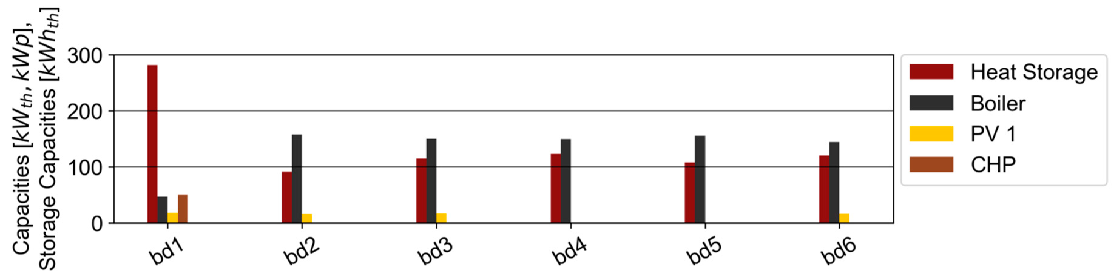
In buildings 2, 3, 4, 5 and 6 (bd2–bd6), the technology system design for the heat supply is similar. A natural gas boiler combined with a heat storage unit is chosen. A PV installation can be found in buildings 1, 2, 3 and 6. The reason for the missing PV in building 4 and 5 is the unfavorable roof orientation.
In Section 3.3.1, Section 3.3.2, Section 3.3.3 and Section 3.3.4, the microgrid optimization will be executed with the time series aggregation approach, as well as the new 2-Level Approach, to compare the results with those from the reference case.

3.3.1. Investigation of Total Annual Costs

The TAC in the 2-Level Approach shows a low deviation of less than 0.1% related to the TAC of the reference case, as shown Figure 4. In the results of the time series aggregation, the deviation is higher in comparison to the 2-Level Approach for the analyzed different typical days. With an increasing number of typical days, the deviation of the time series aggregation related to the reference case decreases, but is still higher than in the 2-Level Approach. The 2-Level Approach shows a significantly lower deviation than the time series aggregation. For all typical periods, the 2-Level-Approach tends to slightly overestimate the TAC, whereas the time series aggregation tends to underestimate it. The reason for the underestimation of the TAC in the time series aggregation approach is the averaging effect caused by the clustering of time series data.

3.3.2. Investigation of Computing Time

The investigation of computing time runs on a Windows desktop PC with an Intel(R) Core(R) i7-6700K @4.00GHz and a Memory of 32 GB RAM.
Figure 5 shows a significantly lower computing time for the 2-Level Approach and the time series aggregation related to the reference case. The 2-Level Approach results in a decrease in the computing time of between −99.72% for 5 typical days and −92.96% for 40 typical days compared to the reference case. The time series aggregation reduces the computing time by −99.97% for five typical days and −93.22% for 40 typical days.
The computing time of the first level in the 2-Level Approach is equal to the time series aggregation because it follows the same approach. The computing time is 51 s for 5 typical days, 315 s for 10 typical days, 2017 s for 20 typical days and 14,754 s for 40 typical days. In addition to the time series aggregation in the first level of the 2-Level Approach, a full-time series optimization is running that results in an overall higher computing time for the 2-Level Approach than for the time series aggregation. The second level of the 2-Level Approach is an LP problem. Thus, the computing time changes only slightly with a minimum of 556 s and maximum of 597 s for solving the second level.

3.3.3. Investigation of the Supply Technologies

The microgrid optimization with full-time series (reference case), time series aggregation and the 2-Level Approach show the same technology structure. To meet the electricity and heating demand, the microgrid optimization opts for boilers, CHPs, heat storages and PV as supply technologies. The investigation of all installed supply technologies in the district is considered in the following paragraphs.
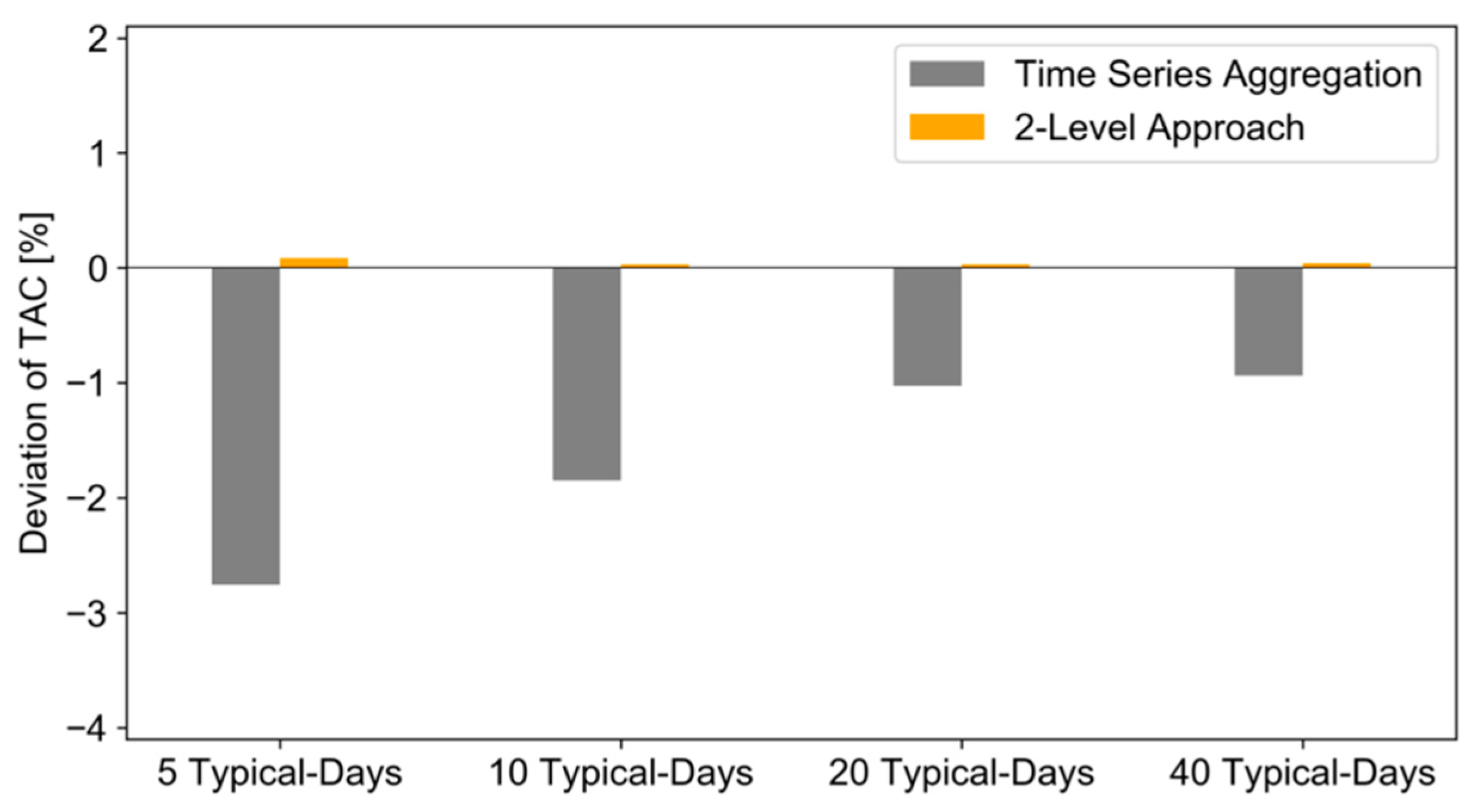
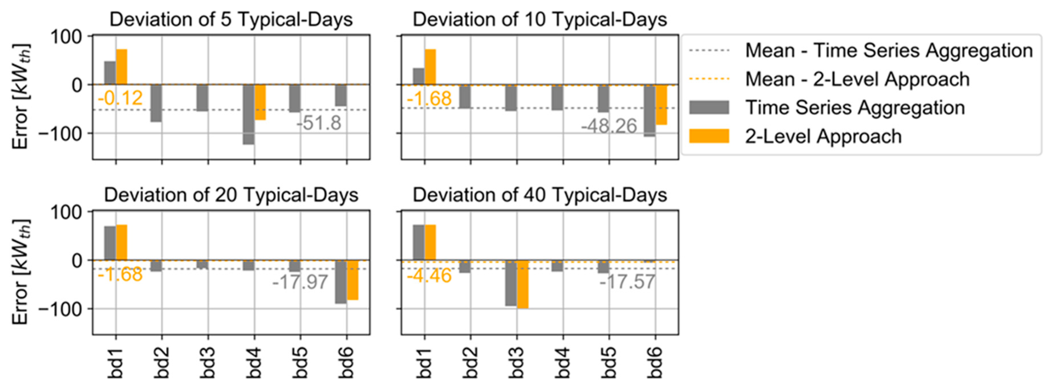
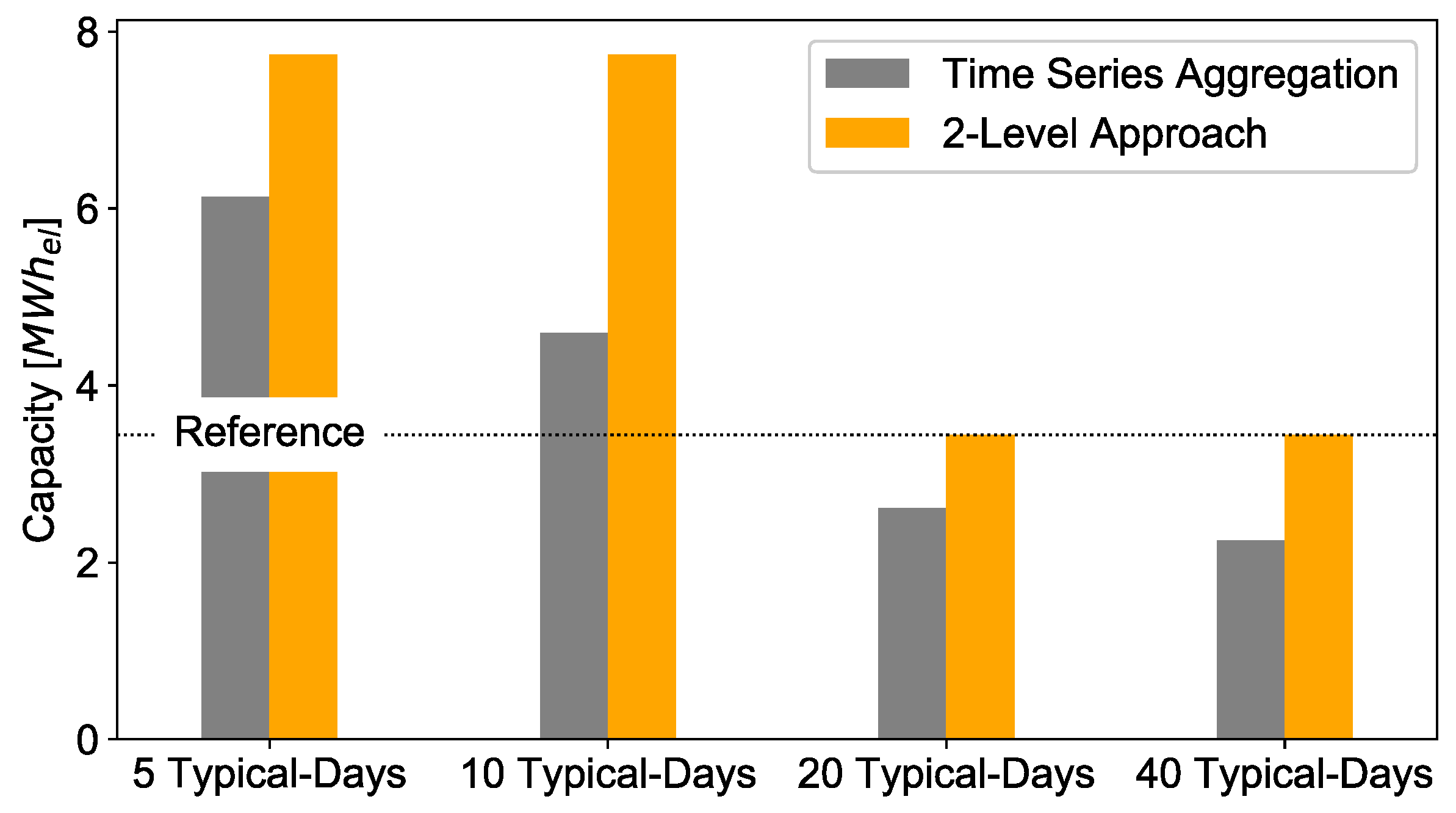
Boiler: The mean deviation of the 2-Level Approach related to the reference case is low, with a maximum of −4.46 kWth in 40 typical days and a minimum of −0.12 kWth in 5 typical days. In the time series aggregation, the mean deviation decreases from −51.8 kWth in 5 typical days to −17.57 kWth in 40 typical days. Thus, the mean results show a significantly lower deviation in the 2-Level Approach than in the time series aggregation.
Figure 6 shows a positive deviation of installed boiler capacities in the case of 5, 10, 20 and 40 typical days for building 1 (bd 1) in the 2-Level Approach. The reason for this pattern is that the CHP in the reference case is installed in building 1, as shown in Figure 3, but in the 2-Level Approach, the CHP is installed in other buildings. A negative deviation of installed boiler capacities is observed in the buildings with additional CHP installation, as shown in Figure 6. Hence, there is a boiler capacity shift based on changing the CHP location. For example, in the 5 typical days case, the boiler capacities decrease in building 3, because the CHP is installed there and, on the other hand, the installed capacities increase in building 1 because of the missing CHP installation in comparison to the reference case.
Moreover, we can observe that the time series aggregation shows a similar pattern to that in the 2-Level-Approach with respect to the CHP-based capacity shifting. The installed capacities increase in building 1 and decrease in the building with the new CHP location. Additionally, there is a trend of high underestimation of boiler capacities in the buildings, which are not part of the changing CHP location. The underestimation of installed capacities decreases with an increasing number of typical days because of more detailed time series data.
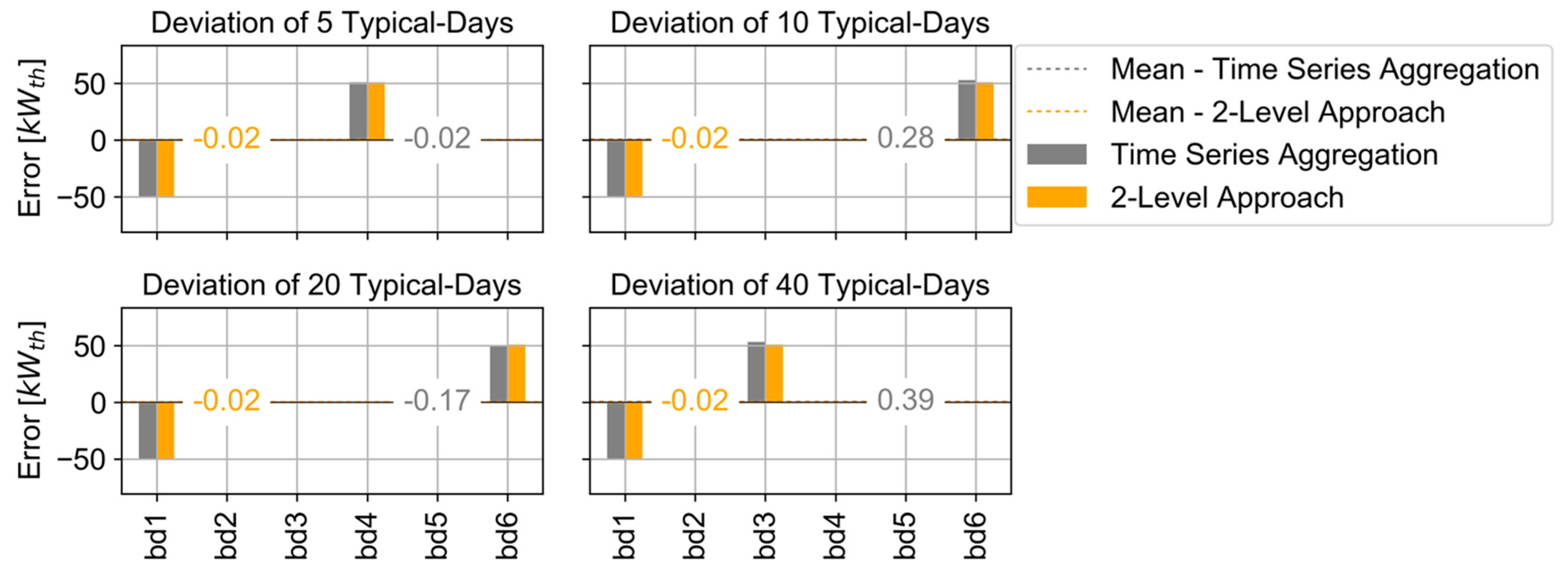
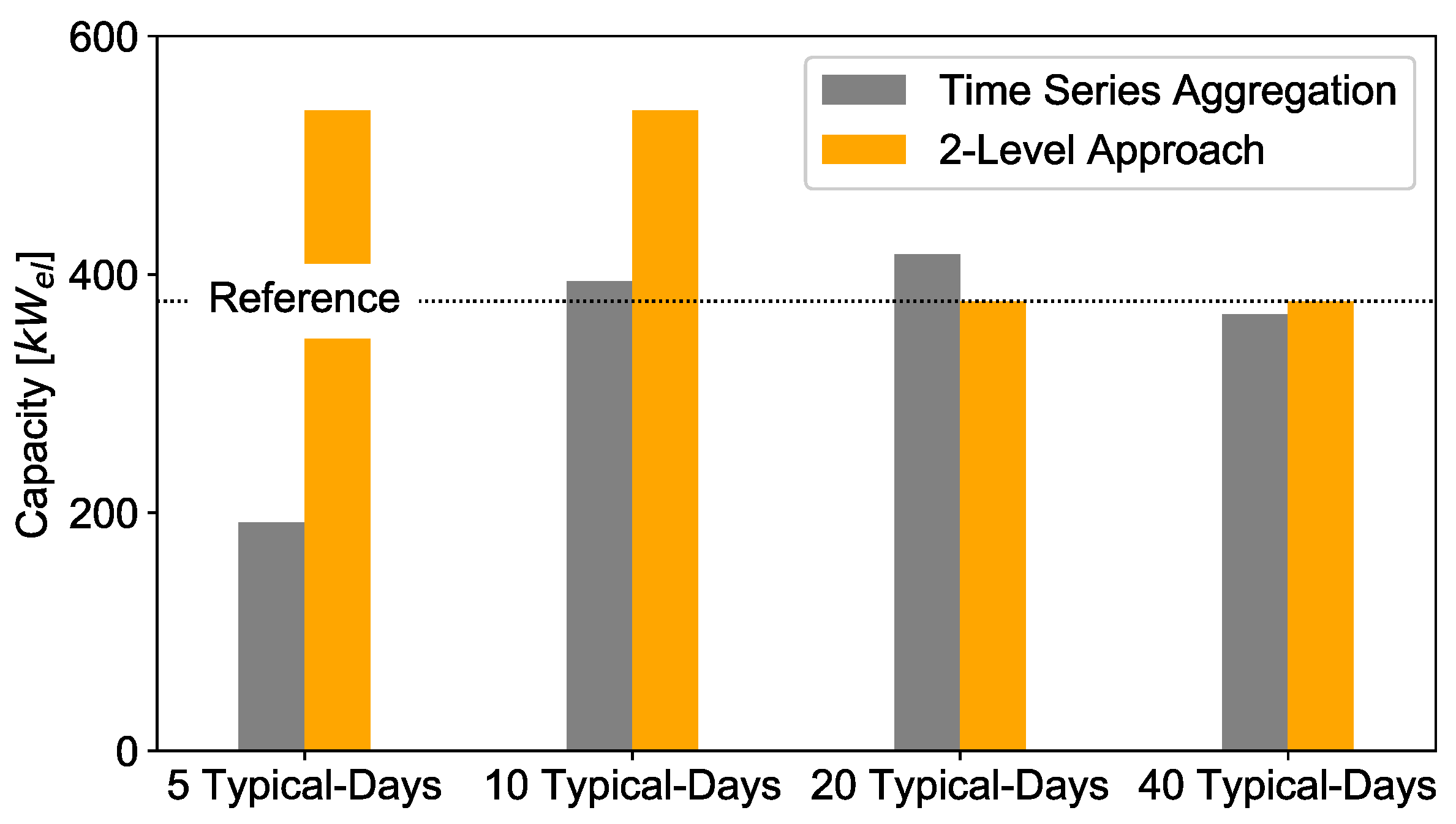
CHP: As discussed in the previous paragraph, the CHP installation location changes between the reference case and the 2-Level Approach, as well as the time series aggregation (see Figure 7). In the case of 5 typical days, the installed CHP shifts from building 1 to building 4, while in the case of 10 and 20 typical days, from building 1 to building 6, and in the case of 40 typical days, from building 1 to building 3.
The mean deviation of the installed CHP capacities computed with the 2-Level Approach is 0.02 kWth for all typical days. The optimization with the time series aggregation results in a minimal deviation of −0.02 kWth for 5 typical days and a maximum of 0.39 kWth for 40 typical days. A possible reason for the building shifting the CHP installation between the different typical days is that the difference in the TAC is not significant. Hence, its location does not affect the TAC. A further analysis is performed in order to investigate the TAC in relation to the location of the CHP in Section 3.3.5.
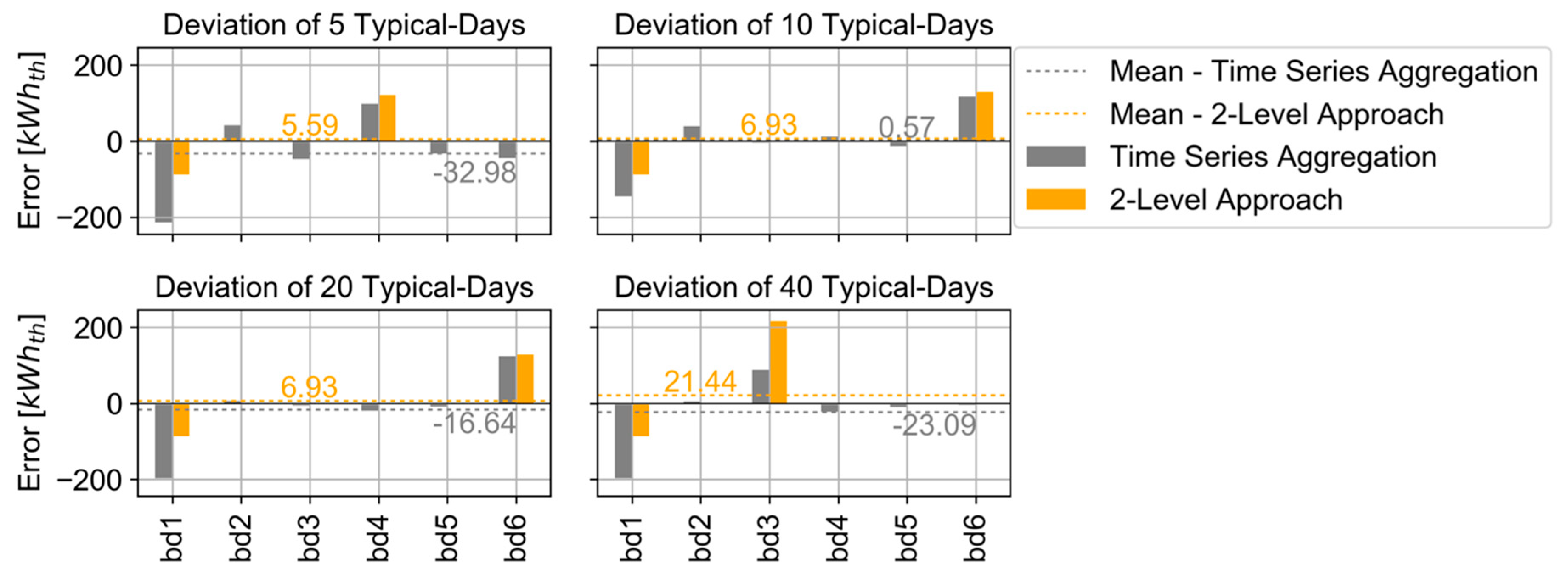
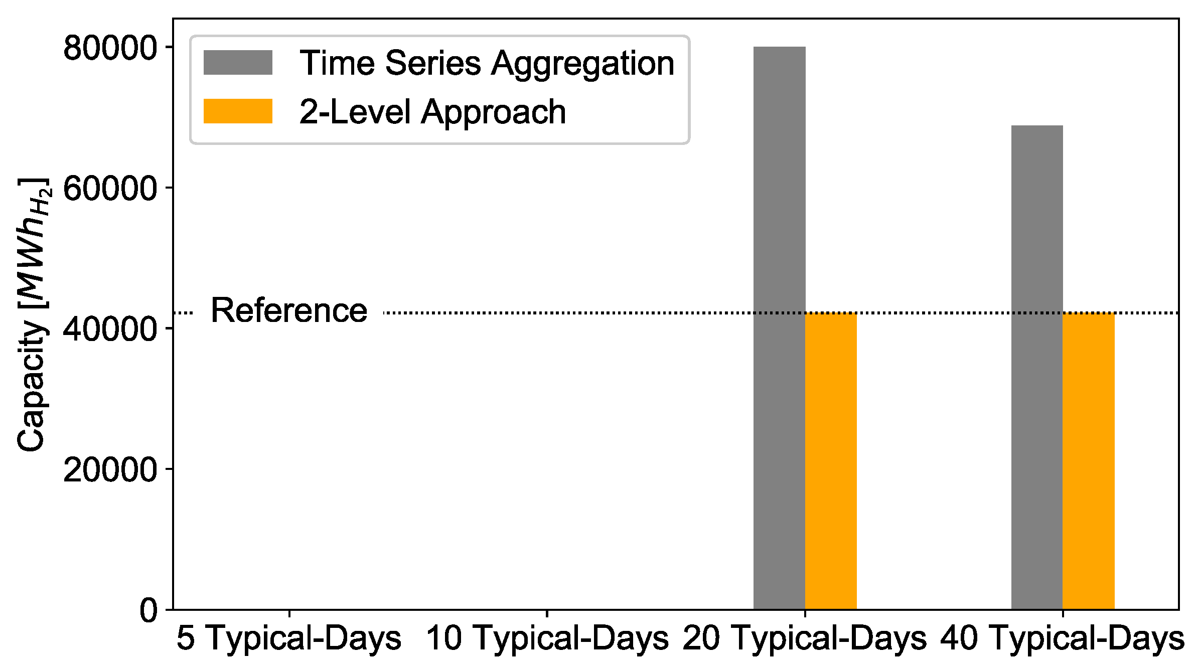
Heat Storage: Comparing the heat storage deviations to the reference case shows that the mean error of installed heat storage capacities changes with the increasing number of typical days, from 5.59 kWh to 21.44 kWh, on the back of the 2-Level Approach. The time series aggregation results exhibit the maximum mean deviation in 5 typical days of -32.98 kWh and the lowest mean deviation in the case of 10 typical days, with 0.57 kWh.
As described in the analysis of boilers and CHPs, the heat storage results also show a clear pattern of capacity shifting between the buildings on the different typical days, especially in the 2-Level Approach, as shown in Figure 8. In the case of 5 and 10 typical days, the installed heat storage capacities decrease in building 1 and increase in building 6, while in the case of 10 and 20 typical days, the installed capacities shift from building 1 to building 6. The possible reason for the same pattern of capacity shifting as in the CHP investigation is that the heat storage supports the operation of the CHP. The electricity generation costs with the CHP are, at 0.26 €/kWh, cheaper than purchasing electricity for 0.2985 €/kWh from the energy provider. Thus, the CHP is preferred by the optimizer to generate electricity, but the thermal energy of the CHP must be used to fulfil the heating demand or store heat in the storage, because an external chiller is not available for the CHP. Hence, the heat storage follows the CHP to buffer excess thermal energy.
The reason for the other typical day’s high deviation of heat storage capacities in 40 typical days is a result of the underestimation of boiler capacities in building 3 for 40 typical days, which does not influence the TAC of the energy supply system.
PV: As well as the 2-Level Approach, the time series aggregation meets the installed PV capacities in the reference case for the different investigated typical periods. Thus, both approaches represent the installed PV capacities very well with no deviation from the reference case.

3.3.4. Investigation of Peak Load

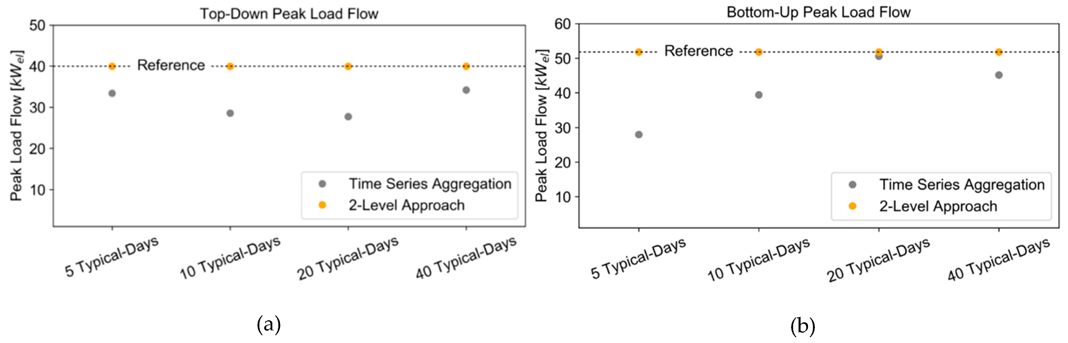
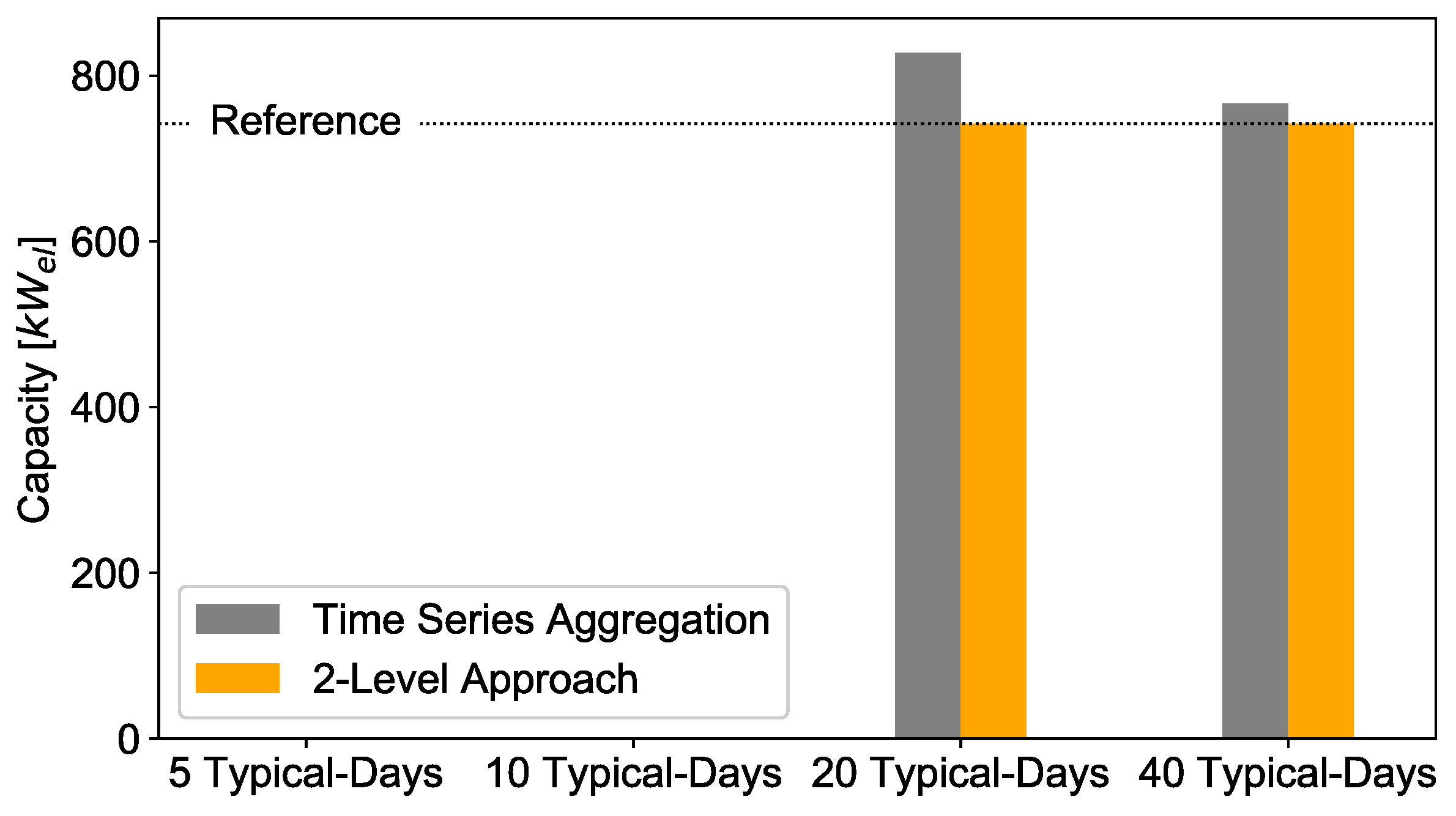
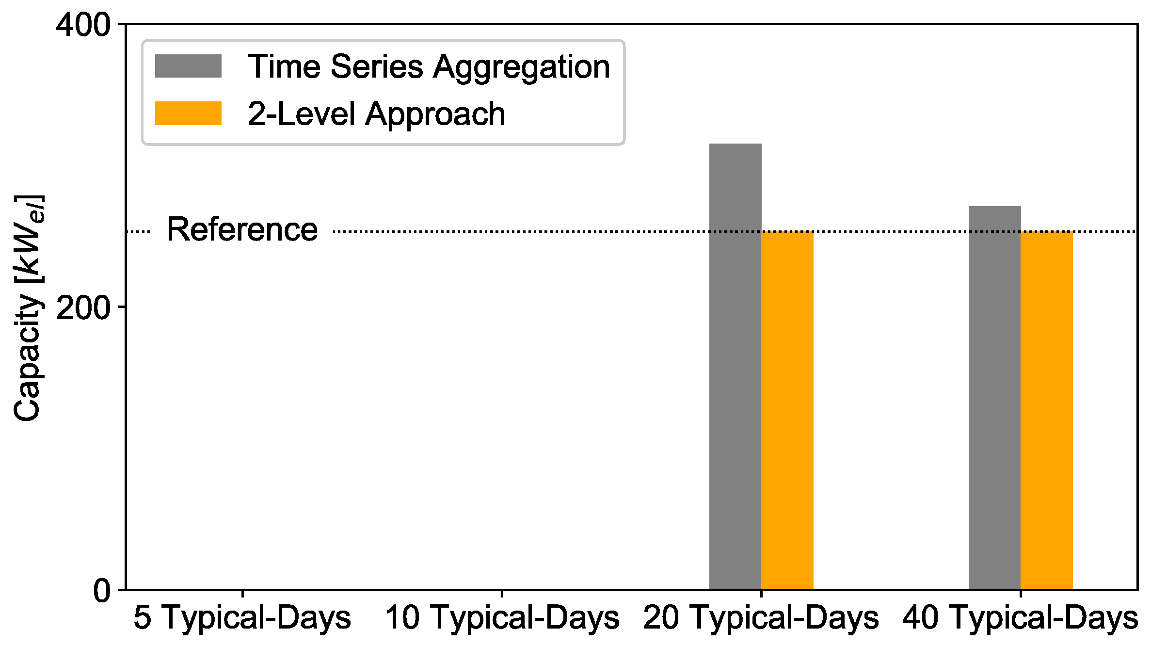
The peak load is the maximum electrical load, which flows over the grid assets. In general, a transformer in a microgrid optimization is the connection between a district and a higher grid level (e.g., between a low voltage and a medium voltage grid). The load flow is divided into two directions: The top-down load flow with the electricity from higher grid level flows via the transformer to fulfil the electricity demand in the district, whereas the bottom-up load flow is defined as the flow from the district (lower) to the higher grid level via the transformer. Bottom-up load flow occurs when the locally produced electricity (e.g., from PV, CHP) exceeds the local electricity demand in the district. The peak load is essential to analyzing the stress of the transformer. Furthermore, voltage issues may become relevant in real grids but are out of scope for this investigation. The peak load investigation is only applied to the electricity grid and not to the natural gas network.
The bottom-up peak load and the top-down peak load of the reference case is very well addressed with the 2-Level Approach, as shown in Figure 9. The time series aggregation underrepresents the peak load for different typical days. Only in the case of 20 typical days in the bottom-up peak load is the result of the time series aggregation close to the reference case. The result is probably based on a coincidence, as it is worse with 40 typical days.
The reason for the underrepresentation of the bottom-up load and top-down load in the time series aggregation is a missing data problem due to the clustering of time series. An increase of the typical days should tend to lead to a more accurate representation of peak periods with the time series aggregation because of the smaller cluster. Also, it is possible to add peak periods to the time series aggregation, which leads to a more accurate solution. On the other hand, adding peak periods leads to an increase in optimization complexity and increasing computing time due to additional time periods. Hence, the investigation shows that the 2-Level Approach is well suited to represent the bottom-up peak load and top-down peak load while the time series aggregation represents it insufficiently.

3.3.5. Impact Analysis of Fixed CHP Position

The investigation of CHPs in Section 3.3.3 showed that only one CHP was installed in one building in the analyzed microgrid energy supply system, but the building location of the CHP installation changes between the different typical days. In the reference case, the CHP was installed in building 1. In the 2-Level Approach, the CHP was installed in building 4 for 5 typical days, in building 6 for 10 and 20 typical days, respectively, and in building 3 for 40 typical days. To investigate the impact of the changing installed CHP location for different typical days, an analysis was performed. In this analysis, the buildings with the installed CHP were fixed one after another to investigate the deviation of TAC related to the reference case. The results of the analysis are shown in 
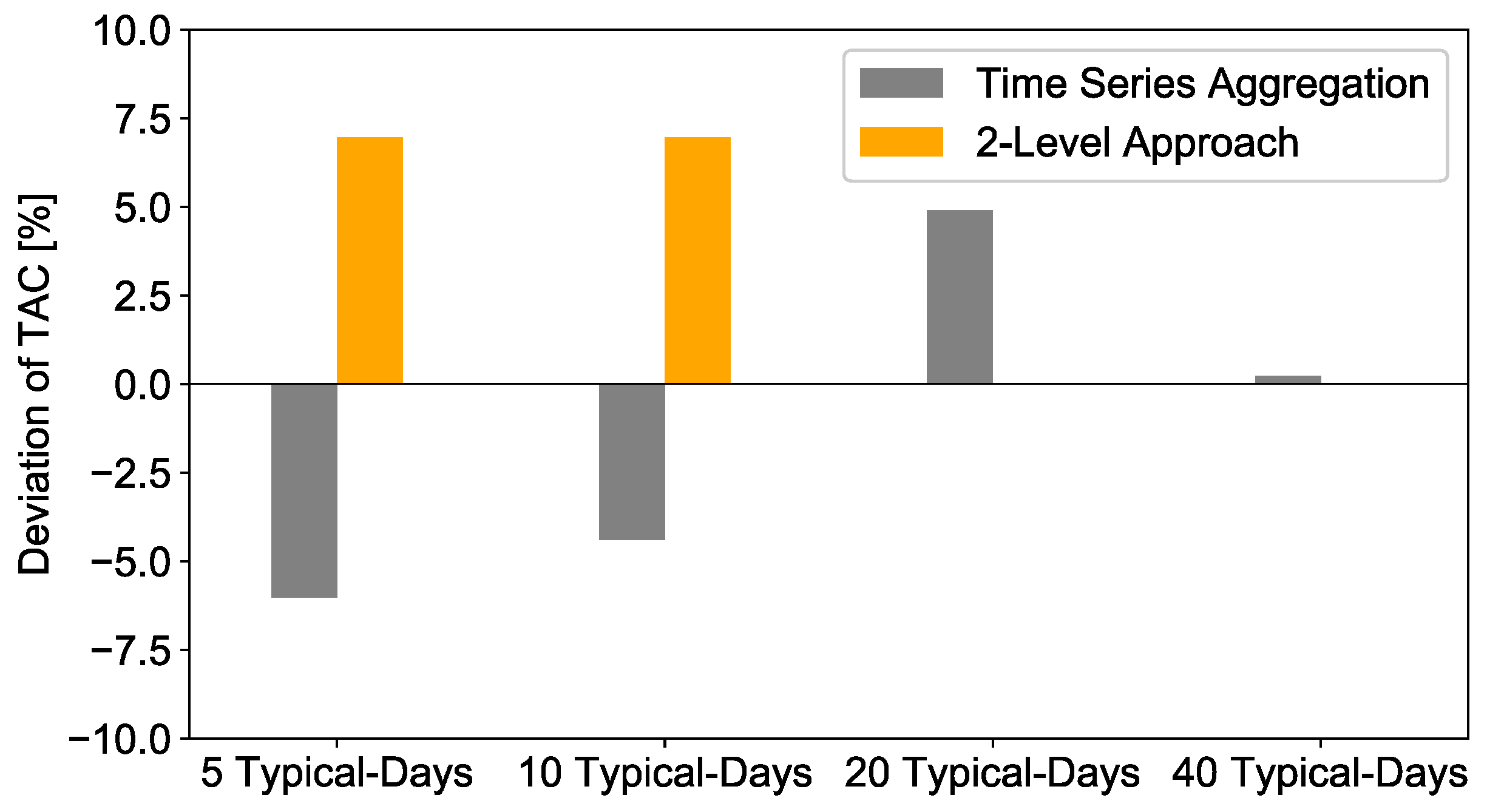
Table 4. Impact of different fix CHP locations on the TAC. On the one hand, the table shows the location of the fixed installed CHP location in columns and, on the other hand, the deviation of the TAC related to the reference case for 5, 10, 20 and 40 typical days.
The analysis shows that the deviation of the TAC for different fixed CHP locations is low compared to the reference case with 0.013% to 0.151%. The lowest deviation of 0.013% can be reached if the CHP is fixed in building 1, which corresponds to the location of the reference case. The highest deviation of TAC is identifiable for a fixed CHP location in building 2, with 0.151% and 10 typical days. However, in general, all results with the fixed location of the CHP show low deviations compared to the reference case. Therefore, the impact of the different placements of CHPs on the TAC is low.
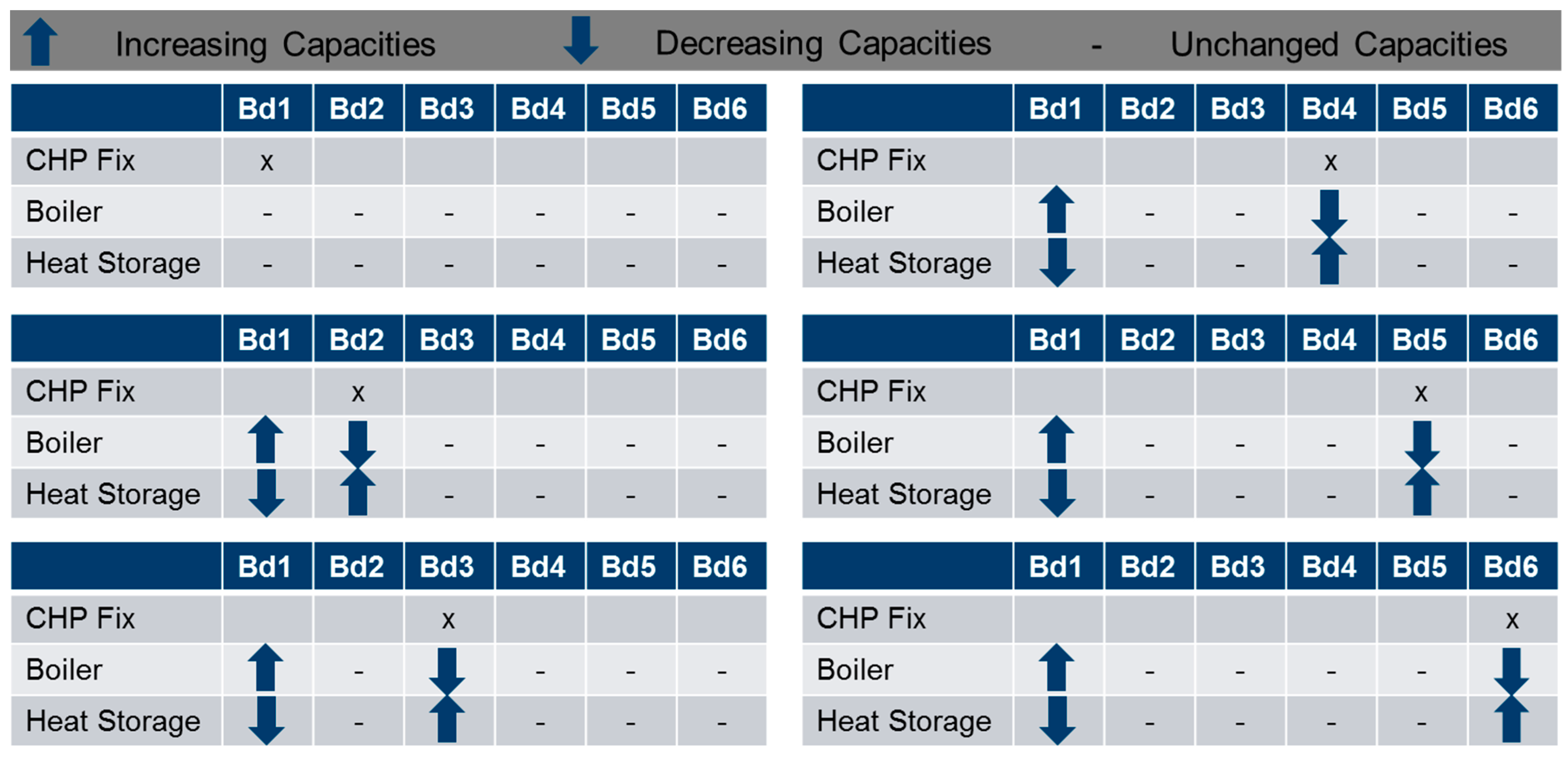
The next pattern of CHP capacity shifting is shown for different fixed CHP locations. The pattern was seen for 5, 10, 20 and 40 typical days. The arrows in Figure 10 represent the trend of installed capacity shifting for the technologies of boilers and heat storage. A dash indicates no changing of installed capacities in comparison to the reference case.
If the CHP is installed in building 1, which is the location of the reference case, there is no changing with respect to the installed capacities for boilers and heat storage. In the other cases of a fixed CHP location, there is a clear pattern that boiler capacities decrease and heat storage capacities increase in the building of the fixed CHP installation. Furthermore, in building 1, the boiler capacities increase, and the heat storage capacities decrease. The reason for increasing boiler capacities in building 1 is that the thermal capacities of the CHP are missing.

4. Second Case Study—Island System

The second study focuses on the application of the presented 2-Level Approach on a simple single-node island system with two commodities, namely electricity and hydrogen. The island system consists of a wind farm, photovoltaics and a small backup plant as the energy supply, and a single electricity demand. Moreover, two alternative energy storage technologies are included: The first stores electricity directly using batteries, while the second uses electrolyzers and fuel cells to store the surplus energy from the electrical grid in hydrogen pressure vessels [60] using electrolysis.

4.1. Data Basis

The regional electricity demand is the ENTSO-E profile of Germany in 2013 normalized to a peak load of 1 MW and is, as well as the wind feed-in, drawn from Robinius et al. [61]. This is only an indication for the purpose of illustration, since real grids of about 1 MW do not have industrial base loads in their profile. The potential photovoltaic feed-in is simulated with PV-Lib [62]. The power plant’s total feed-in is restricted to 10% of the total energy demand in order to maintain a high share of renewable energy supply. As it has been shown by other authors [13], the CO2 reduction costs grow exponentially with decreasing CO2 emissions. In order to avoid unrealistic surplus capacities of the renewable energy and storage components, and in order to make the hydrogen storages a competitive solution in that system, a maximum total feed-in of 10% by the power plant turned out to be an appropriate percentage. Moreover, this highlights the influence of the presented method on the storage dimensioning if a non-sufficient number of typical days is chosen in the first level. The system is shown in Figure 11. Moreover, the modeling of seasonal storages as proposed by Kotzur et al. [37] is also taken into account, which is especially important for the hydrogen storage.

4.2. Technology Portfolio

The detailed input parameters used for modeling the island system model can be taken from Table 5 and are derived from Kotzur et al. [37] with an interest rate of 4% per year for each component for consistency with the above-presented case study. It is worth mentioning that only the wind farm, the photovoltaics, the electrolyzer and the fuel cell are modeled with binary variables according to a certain starting investment (named CAPEXFix in the tables) and fixed operation costs (OPEXFix) depending on the decision as to whether these units are chosen (1) or not (0). In contrast to that, the backup plant, the battery and the hydrogen storage are modeled linearly, since their overall costs only depend on their consumed commodity (gas with 20 ct/kWh in case of the backup plant) and their capacities, respectively. This fairly simple layout is chosen to emphasize the big impact of the proposed 2-Level Approach on the computing time even for small systems while maintaining good results. Additionally, a single-node model with a high share of renewable energy was chosen to highlight the impact of the proposed method on seasonal storages while neglecting balancing effects of multi-regional distribution grid modeling.

4.3. Results of the Second Case Study

The following section focuses on the optimization results of the island system presented above. The following sections first investigate the total annual cost as the actual objective function of the optimization, the computing times to highlight the benefits of the 2-Level Approach followed by a detailed analysis of the component’s capacities within the different levels of the proposed approach.

4.3.1. Investigation of Total Annual Costs

The deviation of the total annual costs depending on the number of typical days and the level in which they are determined by the optimization, in comparison to the reference case that uses the full time series, as well as all four binaries as variables, is illustrated in Figure 12.
As mentioned above, optimization based on 5 or 10 typical days using hierarchical clustering of the daily duration curves leads to a negligence of the hydrogen technologies that ultimately results in higher total annual costs for the whole system after the second optimization. This can be attributed by the fact that the clustering algorithm has a big impact on the smoothness and variance of the clustered input data. In the case of the first level of the optimization using 5 or 10 typical days, this leads to an underestimation of the total variance of the input time series, which means that the time series is considered to be highly repetitive and the overall variance is not kept which has an impact on the design of surplus capacities. Since the fuel cell and the electrolyzer have a start investment of 100,000 € each before building any capacities at all, the optimization based on the aggregated time series turns out to be more profitable if the hydrogen storage technology is not chosen. Because of the fact that the binary variables from the first level of optimization are used as input parameters for the second level of optimization, the hydrogen technologies are not implemented as well when repeating the optimization with the full time series. This turns out not to be a sufficient assumption, since the overall costs of the energy system based on batteries as the only storage technology exceeds the total annual costs of the reference case by approximately 7%.
20 typical periods seem to be sufficient to find the right combination of binary variables, which means that all technologies with binary variables, namely wind, PV and hydrogen technologies, are chosen according to the reference case. This reduces the deviation of the total annual costs compared to the reference case to zero after the second level of optimization. This can also be observed for 40 typical days. However, it needs to be highlighted that in this case the deviation of the total annual costs after the first level of optimization is already far below 1%, which raises the question as to whether the second level of optimization is necessary at all in this case. Last but not least, it needs to be stated that the number of clusters for finding a good set of binary variables is a highly non-trivial question and that it is not guaranteed that the set of binary variables found in the first level always remains the same when choosing more than 20 typical days. However, the chance of finding the cost-optimal set of binary variables becomes more and more likely when increasing the number of typical days.

4.3.2. Investigation of Computing Time

The investigation of the total computing time is illustrated in Figure 13. Here, the computing time for the first level of optimization, labelled by “Time Series Aggregation”, and the total computing time for the 2-Level Approach including the optimization time for the first and second level, but excluding the calculation time for the clustering, which turned out to be negligibly (<0 s) small, are compared with the reference calculation time. For the optimization of the island system, an Intel Core i7 processor was used with eight cores, 16 GB of RAM and a CPU at 3.04 GHz was used. Gurobi 8.1.0 was executed using 6 threads to solve the problem.
First of all, a monotonic rise of the computing time can be observed for an increase of typical days during the first level of the optimization which is trivial because of the growing number of input variables when representing a long time series by more and more representative time steps. However, the overall computing time of the 2-Level Approach depends, in our case, more strongly on the second optimization which becomes more demanding when the hydrogen technologies are included for 20 or 40 typical days, which is crucial for achieving the cost-optimal solution. In these cases, the calculation time for the reference case with 271 s is still 7.2 and 5.3 times bigger than the calculation times for 20 typical days with 38 s and 40 typical days with 51 s respectively. However, when comparing this result in the calculation time of the first level of optimization using 40 typical days with a final deviation of the total annual cost with well below 1%, it becomes obvious that it outperforms all other methods, with 23 s, by more than 35%. Therefore, it is highly important to predefine the targets of the optimization before using the proposed 2-Level Approach, since a simple clustering method with a sufficient number of clusters might be more adequate in some applications.

4.3.3. Investigation of the Different Technology Capacities

Photovoltaic: The photovoltaic capacities depending on the choice of the number of typical days and the different levels are shown in Figure 14. Here, the dotted line represents the capacity of the reference case.
As was discussed above, the representation of the time series by 5 or 10 typical days leads to the negligence of the hydrogen technologies and simultaneously to an overestimation of the redundancy of the time series which means that the clustered time series have a too regular pattern to come close to the real cost-optimal solution. For photovoltaics, this leads to an overestimation of the capacities, especially in the first level of the optimization. This effect is overcome when repeating the calculation with the full time series. However, a higher share of photovoltaics is still needed to compensate the lack of hydrogen storage. For 20 or 40 typical days both optimizations already approach the reference case in the first level and the results are identical for the second case.
Wind energy: The wind energy capacities depending on the choice of the number of typical days and the different levels are shown in Figure 15.
In contrast to the photovoltaic capacities, the wind energy capacities are underestimated in the first level for 5 or 10 typical days. However, when repeating the optimization with the full time series, the capacities are overestimated for 10 typical days and in contrast to the photovoltaics, the wind energy is more favored when using the full time series. This is due to the fact that wind profiles do not have a strong daily pattern and do not strongly correlate with photovoltaics when they are not clustered together with a small number of typical days. For 20 or 40 typical days, the 2-Level Approach meets the results of the reference case. This means that a higher number of clusters do not necessarily improve the clustering process itself if the values are sorted before on a daily basis if they do not have a daily pattern.
Backup plant: The backup plant capacities, depending on the choice of the number of typical days and the different levels, are shown in Figure 16.
Taking into account that the yearly amount of electricity produced by the backup plant is limited to 10% of the overall electricity production, it becomes clear that clustering with too few typical days leads to an underestimation of the capacities because extreme periods are widely neglected and the backup plant is working on a more regular basis with a lower peak load. This is the case for 5 typical days. However, since medoids are chosen as representatives in the used hierarchical clustering algorithm, this is not a strict rule, as it can be observed for 10 and 20 typical days. Concerning the second level of optimization, the missing hydrogen technologies for 5 and 10 typical days lead to a remarkable higher capacity of the backup plant, even in comparison to the reference case. Firstly, the full time series takes all extreme periods into account and secondly the residual loads that cannot be met by wind energy, PV and the battery are considerably higher.
Hydrogen technologies: The capacities of the hydrogen technologies are shown in Figure 17, Figure 18 and Figure 19. Since they are an additional supply line that is used for temporarily storing the energy from the electricity grid only, it is clear that all three units correlate with each other. Since the electrolyzer and the fuel cell have a fixed investment each in contrast to the battery, the hydrogen technologies are not built for 5 and 10 typical days due to the averaging effect of clustering, but are overestimated for 20 and 40 typical days due to the small price per capacity. However, the greater the number of typical days, the more the capacities converge to the reference case. Since the setup of the binary variables for 20 and 40 typical days is identical to the reference case, the 2-Level Approach leads to identical solutions in these cases.
Battery:Figure 20 shows the battery capacities of this study, which turn out to be significantly smaller than the hydrogen capacities by one magnitude if the hydrogen technologies are chosen to be built.
For 5 and 10 typical days used for the initial optimization, an overestimation of the battery capacities can be observed, since the hydrogen technologies are not chosen to store energy from the electricity grid. The reason for that can be derived when comparing the capacities in the first level to those in the second level: Because of the negligence of extreme periods when using few typical days and because of the overestimation of the regularity of inter-daily patterns, smaller storage capacities seem to be sufficient compared to the optimizations that use the full time series. This rule also applies for the cases when the hydrogen technologies are chosen to be built. In these cases, the capacities for the battery storage using typical days are smaller than in the reference case, whereas the reference capacities are met after the second level of optimization.

4.3.4. Investigation of the Connection between the Storages

Although the amount of stored energy in the hydrogen storage and the battery storage depends on the efficiencies of the fuel cell and the discharge efficiency of the battery, it can be stated that the amount of energy that is stored in the hydrogen storage exceeds that of the battery by about one magnitude. However, it can be observed that both storages correlate in a negative manner with respect to their deviations from the reference case within the first level of optimization. When the battery storage is underestimated, the hydrogen storage is overestimated, and vice versa. In addition, the battery storage works on a daily basis, while the hydrogen storage stores energy for longer periods of time, which is illustrated in the color plots in the Appendix A (Figure A1 and Figure A2).
Last but not least, it has to be mentioned that the optimization using the 2-Level Approach results in the same total annual cost minimum as the reference case but in a slightly different operation of the different units. This is also shown in Figure 21.
As can be seen, the black line representing the reference case slightly differs from the output of the 2-Level Approach. However, this is a typical result for energy system optimizations with several alternative technologies since it results in a feasible region that is flat and sometimes even indifferent towards different solutions in its optimum.

5. Summary and Conclusions

MILP microgrid optimization models have a high degree of complexity and thus the requisite computing time is a limitation for solving multi-node systems. To reduce the complexity of the models, techniques like spatial or temporal aggregation can be used. Time series aggregation is a common approach to decrease the temporal resolution by clustering typical time periods. The problem with time series aggregation is the underestimation of the optimization results and the lack of representation time series, e.g., underestimation of the peak load.
This paper investigates a new 2-Level Approach based on time series aggregation to decrease the optimization complexity compared to a full optimization and increase the accuracy compared to a design only based on aggregated time series. The investigation was exemplarily performed for a MILP microgrid energy supply system with six multifamily houses, as well as for a hypothetical island system with a high share of renewable energy, which shows that a transfer of the approach to other energy systems is conceivable.
The results of the first case study show that the 2-Level Approach represents the installed technology capacities accurately, as well as the top-down and bottom-up peak load periods, compared to the reference case. The computing time is lower for the 2-Level Approach compared to the reference case with a maximal decrease of −99.72% for 5 typical days and a minimal decrease of -92.96% for 40 typical days. The TAC is represented very well with the 2-Level Approach, with a deviation of a maximum of 0.08% compared to the reference case. The location of the installed technologies changes between the buildings inside the district for different typical days in the 2-Level Approach, but does not affect the TAC. Thus, a high sensitivity related to the technology placement can be assumed. The aggregated installed capacities over all the buildings in the district change slightly in the 2-Level Approach, while the time series aggregation shows a significantly higher deviation, especially for the installed boiler capacities.
For the second case study, different results with respect to the impact of the binary variables can be observed, but the overall benefit in computing time of the 2-Level Approach remains. Firstly, the island system is smaller and less complex and has only four binary variables. Yet, their influence is significant: for 5 and 10 typical days, the hydrogen technologies for storing energy from the electricity grid are neglected, which results in an overestimation of the TAC of approximately 7% compared to the reference case. However, the decrease in the calculation time is 98.82% and 97.75%, respectively. For 20 and 40 typical days, the set of binaries is identical to the one in the reference case, which reduces the deviation of the TAC to 0%. However, the decrease in computing time is reduced to 86.06% and 81.27%, respectively. This is why 20 typical days is the most appropriate number for optimizing this energy system (second case study) in an exact but computationally tractable manner. However, the strong impact of the number of typical days that must be chosen in the first level to lead to sufficient binary variables among rival storage technologies is also shown by this case study.
Finally, the comparison of both case studies illustrates that the sensitivity of the component selection (i.e., the binaries set) depends on the number of components and their financial similarity: The more similar two components are in terms of their total annual costs and operational behavior, the less the TAC depends on either design. This means that a higher number of typical periods must be chosen to achieve the same energy system design as in the reference case.
In summary, the results of this study show a high degree of accuracy for the 2-Level Approach. Hence, it is possible to optimize large, multi-node energy systems, in which optimization with the full-time series would not be applicable. With the 2-Level Approach, an investigation of a detailed technology operation, including long-term storage, is achievable with high accuracy and acceptable computing time. Furthermore, e.g., the transformer load of a district can be analyzed for different scenarios, which is important for distribution grid network planning. The question of a sufficient time series aggregation for generating a good initial solution remains a task for future research, as well as the application of the proposed method on MILPs that contain piecewise linear functions with more than one binary variable per component.

Author Contributions

Conceptualization: T.K., M.H. and P.S.; Methodology: T.K., M.H., L.K.; Formal analysis: T.K. and M.H. Writing—original draft: T.K. and M.H.; Writing—review & editing: L.K., P.S., F.S., K.P., S.N. and M.R.; Supervision: P.S., L.K., M.R., D.S. Project administration: K.P. and P.S.; Funding acquisition: D.S. and M.R.

Funding

The first author would like to thank Westnetz GmbH for their cooperation and funding. Additionally, the Helmholtz Association under the Joint Initiative “EnergySystem 2050—A Contribution of the Research Field Energy” supported this work. In addition, the authors acknowledge the financial support by the Federal Ministry for Economic Affairs and Energy of Germany in the project METIS (project number 03ET4064A).

Conflicts of Interest

The authors declare no conflict of interest.

Appendix A. Load Profiletable

The aggregated electricity and heating demand profiles are shown in Figure A3 and Figure A4. For instance, the month of January is presented for electricity and heating demand in Figure A5 and Figure A6. Figure A1 and Figure A2 show the state of charge of the battery storage and the hydrogen storage for 40 typical days. This reveals that the framework is capable of taking seasonal storage into account, which is the case for the hydrogen storage, whereas the optimized battery stores energy on a daily basis.
Figure A1. Case study 2—Battery storage operation for 40 typical days (level 1).
Energies 12 02825 g0a1
Figure A2. Case study 2—Hydrogen storage operation for 40 typical days (level 1).
Energies 12 02825 g0a2
Figure A3. Case study 1—Aggregated heating load profile for six buildings.
Energies 12 02825 g0a3
Figure A4. Case study 1—Exemplary heating load profile for January.
Energies 12 02825 g0a4
Figure A5. Case study 1—Aggregated electricity load profile for six buildings.
Energies 12 02825 g0a5
Figure A6. Case study 1—Exemplary electricity load profile for January.
Energies 12 02825 g0a6

Appendix B. Demand Characterization

An overview of the total demands and the PV generation potentials as a result of the preprocessing is given in Table A1. The bottom-up approach in the load profile simulation leads to different total electricity and heating demands for the individual buildings (multi-family houses). The highest electricity demand in the district is shown in building 3, with 24,892 kWh, while the lowest is in building 4, at 17,439 kWh. The highest peak load of individual buildings is in building 1, with 22.97 kWh and, after that, 22.05 kWh in building 3.
The building parameter and shape of the individual multi-family houses are similar. Thus, the installable PV capacities are in a range between 16.16 kWp in building 5 and 17.88 kWp in building 3. The roofs of the buildings are divided into two areas, roof 1 and roof 2.
The heating demand has the highest value in building 6, with 213,360 kWh, and the lowest in building 2, at 211,961 kWh. The peak heating demand is the same for all individual buildings with 200.27 kWh due to identical building parameters and weather conditions.
Table A1. Yearly electricity and heat demand and PV potential per building.
BuildingsBd1Bd2Bd3Bd4Bd5Bd6
Electricity demand [kWh]24,71819,40924,89217,43923,31019,718
Heating demand [kWh]213,008211,961212,160212,865212,987213,360
PV potential roof 1 [kWp]16.4216.4517.8817.2716.1616.63
PV potential roof 2 [kWp]16.4216.4517.8817.2716.1616.63
Construction Year196519651965196519651965
Building TypeMulti-Family HouseMulti-Family HouseMulti-Family HouseMulti-Family HouseMulti-Family HouseMulti-Family House

References

  1. Hirsch, A.; Parag, Y.; Guerrero, J. Microgrids: A review of technologies, key drivers, and outstanding issues. Renew. Sustain. Energy Rev. 2018, 90, 402–411. [Google Scholar] [CrossRef]
  2. Schütz, T.; Hu, X.; Fuchs, M.; Müller, D. Optimal design of decentralized energy conversion systems for smart microgrids using decomposition methods. Energy 2018, 156, 250–263. [Google Scholar] [CrossRef]
  3. Obara, S.Y.; Sato, K.; Utsugi, Y. Study on the operation optimization of an isolated island microgrid with renewable energy layout planning. Energy 2018, 161, 1211–1225. [Google Scholar] [CrossRef]
  4. Vafaei, M.; Kazerani, M. Optimal Unit-Sizing of a Wind-Hydrogen-Diesel Microgrid System for a Remote Community. In Proceedings of the IEEE Trondheim PowerTech, Trondheim, Norway, 19–23 June 2011; pp. 1–7. [Google Scholar]
  5. Mashayekh, S.; Stadler, M.; Cardoso, G.; Heleno, M. A mixed integer linear programming approach for optimal DER portfolio, sizing, and placement in multi-energy microgrids. Appl. Energy 2017, 187, 154–168. [Google Scholar] [CrossRef] [Green Version]
  6. Mehleri, E.D.; Sarimveis, H.; Markatos, N.C.; Papageorgiou, L.G. Optimal design and operation of distributed energy systems: Application to Greek residential sector. Renew. Energy 2013, 51, 331–342. [Google Scholar] [CrossRef]
  7. Akbari, K.; Jolai, F.; Ghaderi, S.F. Optimal design of distributed energy system in a neighborhood under uncertainty. Energy 2016, 116, 567–582. [Google Scholar] [CrossRef]
  8. Basu, A.K.; Chowdhury, S.P.; Chowdhury, S.; Paul, S. Microgrids: Energy management by strategic deployment of DERs-A comprehensive survey. Renew. Sustain. Energy Rev. 2011, 15, 4348–4356. [Google Scholar] [CrossRef]
  9. Morvaj, B.; Evins, R.; Carmeliet, J. Optimization framework for distributed energy systems with integrated electrical grid constraints. Appl. Energy 2016, 171, 296–313. [Google Scholar] [CrossRef]
  10. Morvaj, B.; Evins, R.; Carmeliet, J. Decarbonizing the electricity grid: The impact on urban energy systems, distribution grids and district heating potential. Appl. Energy 2017, 191, 125–140. [Google Scholar] [CrossRef]
  11. Omu, A.; Choudhary, R.; Boies, A. Distributed energy resource system optimisation using mixed integer linear programming. Energy Policy 2013, 61, 249–266. [Google Scholar] [CrossRef]
  12. Yang, Y.; Zhang, S.; Xiao, Y. Optimal design of distributed energy resource systems coupled with energy distribution networks. Energy 2015, 85, 433–448. [Google Scholar] [CrossRef]
  13. Gabrielli, P.; Gazzani, M.; Martelli, E.; Mazzotti, M. Optimal design of multi-energy systems with seasonal storage. Appl. Energy 2018, 219, 408–424. [Google Scholar] [CrossRef]
  14. Helal, S.A.; Najee, R.J.; Hanna, M.O.; Shaaban, M.F.; Osman, A.H.; Hassan, M.S. An energy management system for hybrid microgrids in remote communities. In Proceedings of the IEEE 30th Canadian Conference on Electrical and Computer Engineering (CCECE), Windsor, ON, Canada, 30 April–3 May 2017; pp. 1–4. [Google Scholar]
  15. Olivares, D.E.; Cañizares, C.A.; Kazerani, M. A Centralized Energy Management System for Isolated Microgrids. IEEE Trans. Smart Grid 2014, 5, 1864–1875. [Google Scholar] [CrossRef]
  16. Falke, T.; Krengel, S.; Meinerzhagen, A.-K.; Schnettler, A. Multi-objective optimization and simulation model for the design of distributed energy systems. Appl. Energy 2016, 184, 1508–1516. [Google Scholar] [CrossRef]
  17. Prousch, S.; Breuer, C.; Moser, A. Optimization of decentralized energy supply systems. In Proceedings of the 7th International Conference on the European Energy Market, Madrid, Spain, 23–25 June 2010; pp. 1–6. [Google Scholar]
  18. Fazlollahi, S.; Girardin, L.; Maréchal, F. Clustering Urban Areas for Optimizing the Design and the Operation of District Energy Systems. Comput. Aided Chem. Eng. 2014, 33, 1291–1296. [Google Scholar] [CrossRef]
  19. Stadler, P.; Girardin, L.; Ashouri, A.; Maréchal, F. Contribution of Model Predictive Control in the Integration of Renewable Energy Sources within the Built Environment. Front. Energy Res. 2018, 6, 22. [Google Scholar] [CrossRef]
  20. Unternährer, J.; Moret, S.; Joost, S.; Maréchal, F. Spatial clustering for district heating integration in urban energy systems: Application to geothermal energy. Appl. Energy 2017, 190, 749–763. [Google Scholar] [CrossRef] [Green Version]
  21. Geidl, M.; Andersson, G. A modeling and optimization approach for multiple energy carrier power flow. In Proceedings of the IEEE Russia Power Tech, St. Petersburg, Russia, 27–30 June 2005; pp. 1–7. [Google Scholar]
  22. Bracco, S.; Dentici, G.; Siri, S. DESOD: A mathematical programming tool to optimally design a distributed energy system. Energy 2016, 100, 298–309. [Google Scholar] [CrossRef]
  23. Haikarainen, C.; Pettersson, F.; Saxén, H. A model for structural and operational optimization of distributed energy systems. Appl. Therm. Eng. 2014, 70, 211–218. [Google Scholar] [CrossRef]
  24. Harb, H.; Schwager, C.; Streblow, R.; Müller, D. Optimal Design of Energy Systems in Residential Districts with Interconnected Local Heating and Electrical Networks. In Proceedings of the Building Simulation Conference, Hyderabad, India, 7–9 December 2015. [Google Scholar]
  25. Jennings, M.; Fisk, D.; Shah, N. Modelling and optimization of retrofitting residential energy systems at the urban scale. Energy 2014, 64, 220–233. [Google Scholar] [CrossRef]
  26. Zhou, Z.; Liu, P.; Li, Z.; Ni, W. Economic assessment of a distributed energy system in a new residential area with existing grid coverage in China. Comput. Chem. Eng. 2013, 48, 165–174. [Google Scholar] [CrossRef]
  27. Domínguez-Muñoz, F.; Cejudo-López, J.M.; Carrillo-Andrés, A.; Gallardo-Salazar, M. Selection of typical demand days for CHP optimization. Energy Build. 2011, 43, 3036–3043. [Google Scholar] [CrossRef]
  28. Kotzur, L.; Markewitz, P.; Robinius, M.; Stolten, D. Impact of different time series aggregation methods on optimal energy system design. Renew. Energy 2018, 117, 474–487. [Google Scholar] [CrossRef] [Green Version]
  29. Pfenninger, S. Dealing with multiple decades of hourly wind and PV time series in energy models: A comparison of methods to reduce time resolution and the planning implications of inter-annual variability. Appl. Energy 2017, 197, 1–13. [Google Scholar] [CrossRef]
  30. Bahl, B.; Kümpel, A.; Seele, H.; Lampe, M.; Bardow, A. Time-series aggregation for synthesis problems by bounding error in the objective function. Energy 2017, 135, 900–912. [Google Scholar] [CrossRef]
  31. Baumgärtner, N.; Bahl, B.; Hennen, M.; Bardow, A. RiSES3: Rigorous Synthesis of Energy Supply and Storage Systems via time-series relaxation and aggregation. Comput. Chem. Eng. 2019, 127, 127–139. [Google Scholar] [CrossRef]
  32. Bahl, B.; Söhler, T.; Hennen, M.; Bardow, A. Typical Periods for Two-Stage Synthesis by Time-Series Aggregation with Bounded Error in Objective Function. Front. Energy Res. 2018, 5, 35. [Google Scholar] [CrossRef]
  33. Yokoyama, R.; Shinano, Y.; Wakayama, Y.; Wakui, T. Model reduction by time aggregation for optimal design of energy supply systems by an MILP hierarchical branch and bound method. Energy 2019, 181, 782–792. [Google Scholar] [CrossRef]
  34. Welder, L.; Ryberg, D.S.; Kotzur, L.; Grube, T.; Robinius, M.; Stolten, D. Spatio-temporal optimization of a future energy system for power-to-hydrogen applications in Germany. Energy 2018, 158, 1130–1149. [Google Scholar] [CrossRef]
  35. Welder, L.; Linssen, J.; Robinius, M.; Stolten, D. FINE—Framework for Integrated Energy System Assessment 2018. Available online: https://github.com/FZJ-IEK3-VSA/FINE (accessed on 1 July 2019).
  36. Kotzur, L.; Markewitz, P.; Robinius, M.; Stolten, D. tsam—Time Series Aggregation Module 2017. Available online: https://github.com/FZJ-IEK3-VSA/tsam (accessed on 1 July 2019).
  37. Kotzur, L.; Markewitz, P.; Robinius, M.; Stolten, D. Time series aggregation for energy system design: Modeling seasonal storage. Appl. Energy 2018, 213, 123–135. [Google Scholar] [CrossRef] [Green Version]
  38. Nahmmacher, P.; Schmid, E.; Hirth, L.; Knopf, B. Carpe diem: A novel approach to select representative days for long-term power system modeling. Energy 2016, 112, 430–442. [Google Scholar] [CrossRef]
  39. Ward, J.H., Jr. Hierarchical Grouping to Optimize an Objective Function. J. Am. Stat. Assoc. 1963, 5, 236–244. [Google Scholar] [CrossRef]
  40. Richardson, I.; Thomson, M.; Infield, D. A high-resolution domestic building occupancy model for energy demand simulations. Energy Build. 2008, 40, 1560–1566. [Google Scholar] [CrossRef] [Green Version]
  41. Richardson, I.; Thomson, M.; Infield, D. Domestic electricity use: A high-resolution energy demand model. Energy Build. 2010, 42, 1878–1887. [Google Scholar] [CrossRef] [Green Version]
  42. Richardson, I.; Thomson, M.; Infield, D.; Delahunty, A. Domestic lighting: A high-resolution energy demand model. Energy Build. 2009, 41, 781–789. [Google Scholar] [CrossRef] [Green Version]
  43. Kemmler, A.; Straßburg, S.; Seefeldt, F.; Anders, N.; Rohde, C.; Fleiter, T.; Aydemir, A.; Kleeberger, H.; Hardi, L.; Geiger, B. Datenbasis Zur Bewertung Von Energieeffizienzmaßnahmen in Der Zeitreihe 2005–2014; Umweltbundesamt: Berlin, Germany, 2017. [Google Scholar]
  44. Holmgren, W.F.; Hansen, C.W.; Mikofski, M.A. pvlib python: A python package for modeling solar energy systems. J. Open Sour. Softw. 2018, 3, 884. [Google Scholar] [CrossRef]
  45. Lindberg, K.B.; Doorman, G.; Fischer, D.; Korpås, M.; Ånestad, A.; Sartori, I. Methodology for optimal energy system design of Zero Energy Buildings using mixed-integer linear programming. Energy Build. 2016, 127, 194–205. [Google Scholar] [CrossRef] [Green Version]
  46. Frauenhofer ISE. Current and Future Cost of Photovoltaics. Long-term Scenarios for Market Development, System Prices and LcoE of Utility-Scale Pv Systems 2015. Available online: https://www.ise.fraunhofer.de/content/dam/ise/de/documents/publications/studies/AgoraEnergiewende_Current_and_Future_Cost_of_PV_Feb2015_web.pdf (accessed on 1 July 2019).
  47. Sterchele, P.; Kalz, D.; Palzer, A. Technisch-ökonomische Analyse von Maßnahmen und Potentialen zur energetischen Sanierung im Wohngebäudesektor heute und für das Jahr 2050. Bauphysik 2016, 38, 193–211. [Google Scholar] [CrossRef]
  48. Streblow, R.; Ansorge, K. Genetischer Algorithmuszur kombinatorischen Optimierung von Gebäudehülle und Anlagentechnik; Gebäude-Energiewende: Berlin, Germany, 2017. [Google Scholar]
  49. Lauinger, D.; Caliandro, P.; Van herle, J.; Kuhn, D. A linear programming approach to the optimization of residential energy systems. J. Energy Storage 2016, 7, 24–37. [Google Scholar] [CrossRef]
  50. ASUE. BHKW-Kenndaten 2014/2015–Module, Anbieter, Kosten; Arbeitsgemeinschaft für sparsamen und umweltfreundlichen Energieverbrauch e.V.: Berlin, Germany, 2015. [Google Scholar]
  51. Rager, J.M.F.; Maréchal, F. Urban Energy System Design from the Heat Perspective Using Mathematical Programming Including Thermal Storage; Thèse École polytechnique fédérale de Lausanne EPFL: Lausanne, Switzerland, 2015. [Google Scholar]
  52. Klingler, A.-L. Self-consumption with PV+Battery systems: A market diffusion model considering individual consumer behaviour and preferences. Appl. Energy 2017, 205, 1560–1570. [Google Scholar] [CrossRef]
  53. Linssen, J.; Stenzel, P.; Fleer, J. Techno-economic analysis of photovoltaic battery systems and the influence of different consumer load profiles. Appl. Energy 2017, 185, 2019–2025. [Google Scholar] [CrossRef]
  54. Figgener, J.; Haberschusz, D.; Kairies, P.K.; Wessels, O.; Tepe, B.; Sauer, U.D. Wissenschaftliches Mess-und Evaluierungsprogramm Solarstromspeicher 2.0—Jahresbericht 2017; Institut für Stromrichtertechnik und Elektrische Antriebe der RWTH Aachen: Aachen, Germany, 2017. [Google Scholar]
  55. Lindberg, K.B.; Fischer, D.; Doorman, G.; Korpås, M.; Sartori, I. Cost-optimal energy system design in Zero Energy Buildings with resulting grid impact: A case study of a German multi-family house. Energy Build. 2016, 127, 830–845. [Google Scholar] [CrossRef] [Green Version]
  56. Bundesnetzagentur Deutschland, Haushaltskundenpreis Strom und Gas/Entwicklungen Beschaffungskosten, Netzentgelte und EEG-Umlage (Stichtag 1. April 2017), 2017. Available online: https://www.bundesnetzagentur.de/SharedDocs/Downloads/DE/Sachgebiete/Energie/Unternehmen_Institutionen/DatenaustauschUndMonitoring/Monitoring/Monitoring2017_Kapitel/E_Einzelhandel2017.pdf?__blob=publicationFile&v=1 (accessed on 1 July 2019).
  57. Bundesnetzagentur Deutschland. EEG-Registerdaten und EEG-Fördersätze; Publications Office of the European Union: Luxembourg, 2017. [Google Scholar]
  58. Bundesministerium der Justiz und für Verbraucherschutz KWKG 2016. Available online: https://www.gesetze-im-internet.de/kwkg_2016/ (accessed on 1 July 2019).
  59. European Energy Exchange AG. Üblicher Strompreis gemäß KWK-Gesetz. Available online: https://www.eex.com/de/marktdaten/strom/spotmarkt/kwk-index/kwk-index-download (accessed on 1 July 2019).
  60. Schiebahn, S.; Grube, T.; Robinius, M.; Tietze, V.; Kumar, B.; Stolten, D. Power to gas: Technological overview, systems analysis and economic assessment for a case study in Germany. Int. J. Hydrogen Energy 2015, 40, 4285–4294. [Google Scholar] [CrossRef]
  61. Robinius, M.; Stein, F.T.; Schwane, A.; Stolten, D. A Top-Down Spatially Resolved Electrical Load Model. Energies 2017, 10, 361. [Google Scholar] [CrossRef]
  62. Andrews, R.W.; Stein, J.S.; Hansen, C.; Riley, D. Introduction to the open source PV LIB for python Photovoltaic system modelling package. In Proceedings of the IEEE 40th Photovoltaic Specialist Conference (PVSC), Denver, CO, USA, 8–13 June 2014; pp. 170–174. [Google Scholar]
Figure 1. Workflow of 2-Level Approach.
Energies 12 02825 g001
Figure 2. Composition of total annual costs in the microgrid optimization model.
Energies 12 02825 g002
Figure 3. Installed capacities in buildings (bd) for reference case with full-time series.
Energies 12 02825 g003
Figure 4. Deviation of total annual costs for different typical days compared to full time series.
Energies 12 02825 g004
Figure 5. Comparison of the computing time.
Energies 12 02825 g005
Figure 6. Deviation of installed boiler capacities with the 2-Level Approach and time series aggregation in buildings (bd) compared to full time series.
Energies 12 02825 g006
Figure 7. Deviation of installed CHP capacities with 2-Level Approach and time series aggregation in buildings (bd) compared to full time series.
Energies 12 02825 g007
Figure 8. Deviation of installed heat storage capacities with the 2-Level Approach and time series aggregation.
Energies 12 02825 g008
Figure 9. Top-down (a) and bottom-up (b) peak load flow of time series aggregation and 2-Level Approach compared to the reference case with full time series.
Energies 12 02825 g009
Figure 10. Changing capacities based on fixed CHP location.
Energies 12 02825 g010
Figure 11. Technology portfolio of the island system.
Energies 12 02825 g011
Figure 12. Deviation of total annual costs for different typical days compared to full time series.
Energies 12 02825 g012
Figure 13. Comparison of the computing time.
Energies 12 02825 g013
Figure 14. Deviation of installed photovoltaic capacities with the 2-Level Approach and time series aggregation compared to full time series.
Energies 12 02825 g014
Figure 15. Deviation of installed wind energy capacities with the 2-Level Approach and time series aggregation compared to full time series.
Energies 12 02825 g015
Figure 16. Deviation of installed backup plant capacities with the 2-Level Approach and time series aggregation compared to full time series.
Energies 12 02825 g016
Figure 17. Deviation of installed electrolyzer capacities with the 2-Level Approach and time series aggregation compared to full time series.
Energies 12 02825 g017
Figure 18. Deviation of installed fuel cell capacities with the 2-Level Approach and time series aggregation compared to full time series.
Energies 12 02825 g018
Figure 19. Deviation of installed hydrogen storage capacities with the 2-Level Approach and time series aggregation compared to full time series.
Energies 12 02825 g019
Figure 20. Deviation of installed battery capacities with the 2-Level Approach and time series aggregation compared to full time series.
Energies 12 02825 g020
Figure 21. Hydrogen storage operation for the 2-Level Approach and the reference case.
Energies 12 02825 g021
Table 1. Overview of optimization approach and considered time series in 2-Level Approach, time series aggregation and the reference case.
ReferenceTime Series Aggregation2-Level Approach
1st LevelMILPMILPMILP
Full-Time SeriesTypical PeriodsTypical Periods
2nd Level--LP
--Full-Time Series
Table 2. State-of-the-art techno-economic technology parameters.
TechnologiesCAPEXCapCAPEXFixOPEXLifetimeEfficiencyBased on Literature
PV1400 €/kWp1000 €1% of CAPEX25-[45,46]
Condensing Boiler100 €/kWth2800 €1.5% of CAPEX2090%[47,48,49]
Heat Pump600 €/kWth5000 €1% of CAPEX20COP = 2[45,47,48]
ICE-CHP1000 €/kWel15,000 €3% of CAPEX2025%el/60%th[48,50]
Heat Storage34 €/kWhth23 €-250,1%/h[48,51]
Battery Storage700 €/kWhel2000 €-150,01%/h[52,53,54]
Table 3. State-of-the-art techno-economic technology parameters.
Interest Rate4%[55]
Household Electricity Price0.2986 €/kWh [56]
Household Natural Gas Price0.0615 €/kWh[56]
PV Feed-In Tariff0.1245 €/kWh[57]
CHP Premium0.08 €/kWh[58]
CHP Index0.0342 €/kWh[59]
Table 4. Impact of different fix CHP locations on the TAC.
CHP Fix Location
Deviation TAC in %Bd1Bd2Bd3Bd4Bd5Bd6
5 Typical Days0.0130.0920.0750.1210.0830.059
10 Typical Days0.0720.1510.0530.0990.1420.041
20 Typical Days0.0130.0920.0530.0990.0830.041
40 Typical Days0.0130.0910.0530.0990.0830.041
Table 5. Unit parameters of the island system derived from Kotzur et al. [37].
CAPEXCap [€/kWp]CAPEXFix [€]OPEXCap [€/kWp]OPEXFix [€]OPEXVar [€/kWh]Efficiency [%]Charge Efficiency [%]Discharge Efficiency [%]Self-Discharge [%/h]Lifetime [a]
Photovoltaic800100081000 20
Wind Energy1000100,0002020000 20
Backup Plant100003000.2 25
Electrolyzer500100,000153000070 15
Fuel Cell1100100,000333000050 15
Battery3000300 96960.0515
Hydrogen Storage150000 901025

