Development of Engine Efficiency Characteristic in Dynamic Working States

Department of Machine Design and Technology, Faculty of Mechanical Engineering and Robotics, AGH University of Science and Technology, al. Mickiewicza 30, 30-059 Krakow, Poland
Energies 2019, 12(15), 2906; https://0-doi-org.brum.beds.ac.uk/10.3390/en12152906
Submission received: 4 July 2019
/
Revised: 24 July 2019
/
Accepted: 26 July 2019
/
Published: 28 July 2019
(This article belongs to the Special Issue Modelling, Simulation and Control of Thermal Energy Systems)
Abstract
:The objective of this paper is to present a new approach to the problem of combustion engine efficiency characteristic development in dynamic working states. The artificial neural network (ANN) method was used to build a mathematical model of the engine comprising the following parameters: Engine speed, angular acceleration, engine torque, torque change intensity, and fuel mass flow, measured on a test bed on a spark ignition engine in static and dynamic working states. A detailed analysis of ANN design, data preparation, the training method, and the ANN model accuracy are described. The paper presents conducted calculations that clearly show the suitability of the approach in every aspect. Then, a simplified ANN was created, which allows a two dimensional characteristic in dynamic states, including 4 variables, to be determined.
1. Introduction
The overall efficiency of the internal combustion engine is one of its most important operational parameters. It directly influences fuel consumption, which is an extremely important factor both for drivers and car manufacturers who have to meet the strict EU regulations [1].
The overall engine efficiency is defined as the quotient of the mechanical power on the flywheel to the power of the fuel injected into the cylinders. It takes into account all losses related to both thermodynamic processes, internal friction mainly among moving parts in the crank and piston system, as well as losses in the alternator drive, the coolant pump, and other accessories.
Currently, the efficiency of internal combustion engines is up to 40% for spark ignition (SI) naturally aspirated engines [2] and up to 36% for SI turbocharged engines [3]. Over the last 20 years, efficiency has grown by about 10%, due to numerous factors. The main ones are as follows: The use of fuel injection systems, modern lubricants, coatings on pistons and cylinders [4], optimization of the valve timing [5], the use of the Atkinson cycle [2], improved fuels, increased compression ratio and many others.
A well-known method for presenting the efficiency of engines is with the specific fuel consumption, which has been used for many years [6]. It represents isolines of specific fuel consumption as a function of engine rotational speed and torque. It illustrates the efficiency of the engine in the whole working range and makes it possible to compare different constructions. An important limitation of this characteristic is the possibility of applying it only to steady states of engine operation, where the rotational speed and torque are constant and the throttle position is fixed. Therefore, its use in simulations of vehicle fuel consumption is dedicated to significant errors, because vehicle engines work dominantly in dynamic working states [7], where energy accumulation in rotating masses, mixture enrichment at throttle opening, and fuel cut off during deceleration significantly influence engine efficiency. Despite this big disadvantage, this characteristic is often used in simulations of vehicle fuel consumption in different driving cycles. However, it can only be used with sufficient accuracy in comparative simulations, e.g., concerning gear ratio selection [8], allowing differences between different constructions to be shown, rather than nominal values of fuel consumption to be calculated.
A technical problem, where many factors that influence other factors can often be solved with the ANN method, which is capable of approximating non-linear relationships based on a data set from performed measurements. The applications of the ANN method for solving engine performance problems are numerous. The authors of Reference [9] have developed dynamic models of the engine, where speed, throttle angle, and angular acceleration are considered as ANN inputs and engine torque and fuel consumption are the outputs. In References [7,10], the author undertook another attempt. The inertia-related engine features are included in the ANN model enabling fuel flow calculation in dynamic states. In contrast with Reference [9], this model includes not only engine speed, torque, and angular acceleration, but also torque increase over time, which is an important factor including air-fuel mixture enrichment. This method is very precise, but no 2D or 3D characteristic was presented, thus a simple and quick assessment of the engine dynamic parameters is impossible in this case. Computational simulations must be performed to obtain engine efficiency for each particular engine working state. In Reference [11], the ANN method was used to predict the exhaust emissions and performance (e.g., brake specific fuel consumption) of a compression ignition engine based on engine load, engine speed, and the percentage of biodiesel fuel derived from waste cooking oil in diesel fuel. Although this article provides relationships between engine speed, load, and performance, it refers only to static working states. Very similar problems and approaches are presented in References [12,13], however, in these cases the fuel blends are as follows: Diethyl ether diesel fuel mixtures and Jatropha biodiesel, respectively. Artificial intelligence can also be used in more sophisticated problems concerning the efficiency of a combustion engine working in a hybrid drivetrain [14]. The literature shows that, apart from the ANN method, other approaches are also possible when solving the problems of engine efficiency (specific fuel consumption). In Reference [15], the authors’ approach was to analytically calculate energy expenditure and fuel consumption, taking into account the instantaneous specific fuel consumption, approximated by two generalized single dimension polynomial functions. The authors of Reference [16] developed a dynamic model based on the static characteristic complemented by a factor including vehicle speed and acceleration. This model provides a closer characteristic to real engine behaviour, however, such an attempt also includes vehicle features such as gear ratios. The authors of Reference [17] used the mean value model representing the engine. A non-linear model includes air flow and engine inertia, however fuel-air mixture composition is assumed constant and values of some efficiencies are assumed, not measured. The authors of Reference [18] invented the new transient fuel consumption model whose basic structure is steady-state estimation plus transient correction, including engine speed and torque change resulting from the instantaneous speed and acceleration of the vehicle in specific driving cycles.
The need to reduce research costs and shorten the time of prototype preparation leads to the use of computer simulations to the widest possible extent. This, in turn, involves the need to develop more and more accurate mathematical models that reflect the physical construction as closely as possible. The above examples present different approaches to the problem of combustion engine efficiency and the use of different calculation methods. Unfortunately, the development of a graphic representation of combustion engine efficiency in dynamic states is complex, because it requires a multidimensional relationship to be developed. Taking the above into consideration, the author used the ANN to develop a novel method that allows graphical representations to be created with the highest possible match with measurement data from dynamic engine working states.
The rest of the manuscript is organized as follows. Section 2 describes the basics of engine efficiency, including the well-known specific fuel consumption characteristic as well as the problem of engine inertia influencing efficiency in dynamic working states. Section 3 provides information concerning engine tests and the measurement system in static and dynamic states. All the aspects of the ANN (creating mathematical dependency between engine speed, torque, and its efficiency) concerning its architecture, data scaling, and training method, are precisely described. Section 4 presents a novel approach to the problem of drawing engine efficiency in dynamic working states and, finally, shows two dimensional characteristics, allowing engine efficiency to be quickly and precisely calculated. Section 5 presents the simulation results, which prove the correctness of the adopted approach.
2. Problem Formulation
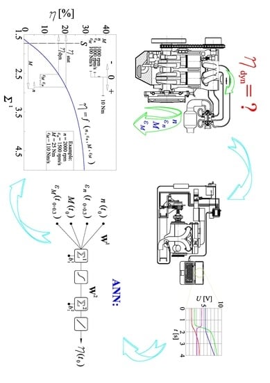
Engine efficiency can be measured for every point in the whole field of work, however, only the maximum values of individual engines are usually given. The efficiency of the engine in the entire work area shows the specific fuel consumption, where, in the coordinate system, torque M vs. the rotational speed n, the contours of specific fuel consumption are presented. Such a characteristic is presented in Figure 1.
The graph in Figure 1 is created based on a method presented in Reference [8], where the algorithm of drawing such a characteristic, based on only 4 operating points, is described in detail. This characteristic can be directly converted to a characteristic of engine efficiency:
where N is the engine power in kW, G is fuel mass flow in g/s, and Wd is the heat value of the fuel in MJ/kg.
As mentioned in the Introduction, these characteristics are based on measurements in static states. In dynamic states, the efficiency of the engine can vary significantly. This results from the following factors: Enrichment of the mixture during load increase (in relation to static states), delay of the system response to the control signal, and accumulation of combustion energy in moving parts of the engine (Figure 2). Although this energy can be partially recovered during deceleration with engine braking, it is usually lost in the form of pumping losses when the throttle is closed and the engine speed is reduced.
It is therefore important to determine the characteristics that, as well as the engine speed n and torque M, also take into account the angular acceleration and the increase in the torque over time, which significantly affect efficiency, as shown in Figure 3.
Such an attempt is strongly desired, because car engines work for a predominant percentage of time in dynamic working conditions, which results from the specificity of road traffic, especially in the area of large urban agglomerations, the impact of road resistance, wind resistance, or the driver’s own operation of the vehicle. It turns out that, in such working conditions, the efficiency of the engine is even smaller. In the WLTP homologation test (Worldwide harmonized light duty vehicle test procedure), the phases in which the engine operates with a constant load are only under 17% of the entire test time. This clearly shows that the use of fuel consumption characteristics in dynamic work states is insufficiently accurate.
3. Methodology
3.1. Measurements in Dynamic Working States
The presented engine efficiency characteristic, using the ANN, is determined based on measurement data from the engine test bench, which allows measurements of the fuel consumption in dynamic operating states to be performed. This is necessary to ensure an appropriate training set for the ANN. Such a set must contain measurement data from all the possible operating states of the engine, covering the entire engine work field, in this case n = 1000–5500 rpm and M = 0–65 Nm. The measurement methodology is described in detail in Reference [7]. Measurements were performed on an SI engine with a displacement of 899 cm3, a nominal power of 29 kW at 5500 rpm, and a nominal torque of 65 Nm at 3000 rpm. Resistant torque was generated by a hydraulically controlled friction brake enabling smooth and rapid load changes (Figure 4). Two parameters, the brake load and throttle opening angle (in the full range 0–90°), were controlled so all the engine working states could be realized. Measurements were performed at a nominal engine temperature. No warm-up period was included. The engine speed was measured with the use of a Tacho GT 3.10 L/405 tachometer. To match the measurement range of the data acquisition device (0–10 V), an additional tooth belt drive, with a ratio of 2.909, was used. The fuel flow was measured indirectly. A Bosch 0 280 217 123 air mass flow meter measured the airflow and an LSU-4.1 Innovate Motorsport LC-1 wideband oxygen sensor (measurement range of λ = 0.5 ÷ 1.523), with a controller, constantly measured the air-fuel ratio. The brake caliper was pivoted and the reaction force was generated by a compression spring, whose shortening was measured by a potentiometer, and a lever system. Such a system measured the moment of resistance, taking into account both the contact pressure between the pads and the disc, as well as the friction coefficient between these elements. The moment of inertia of all elements is known and is taken into account at the stage of building the training set for the ANN. All 4 sensors generated analog voltage signals and were connected to a National Instruments NI USB-6009 data acquisition device. LabVIEW software was used to collect the data on the computer.
All the possible engine states that might occur during normal engine operation in a vehicle must be performed during measurements. All of them are presented in Figure 5.
Figure 5 represents all the situations that might occur during driving. The first one is driving at constant speed on a flat road, the second one is sudden throttle opening—a demand for acceleration, the third one is acceleration with constant torque, the fourth case is engine braking, and the fifth one is slow acceleration with torque and speed increase.
3.2. Data Analysis with the Use of ANN
To use the ANN for measurement data approximation, the ANN architecture, data scaling, transfer functions, and training methods must be defined. The aim is to calculate engine efficiency (resulting from fuel mass flow), which is a function of 4 parameters, as follows: Engine speed n, torque M and angular acceleration εn, and torque increase over time εM. Thus, the considered ANN must have 4 inputs and one output. Only one hidden layer can be used because, with a proper number of hidden neurons, such a network is capable of approximating non-linear relationships with high accuracy [19]. The non-linear function in the hidden layer was set to logsig, which is one of the transfer functions available. It ensures similar results to other functions (e.g., tansig), however, it can be calculated quickly, thus accelerating calculations [19]. Data scaling for all inputs and the output is proportional, because an increase of every single input results in an increase of the output. The ANN used for calculations is presented in Figure 6.
The number of hidden neurons depends on many factors, e.g., the data number (in this case, the training set contained nearly 13,800 data parts from measurements in dynamic and static states), the homogeneity of measurement data, and the method of data scaling, and thus cannot be set up front. The author verified mean squared error (mse) for subsequent numbers of hidden neurons, as presented in Figure 7.
The mse decreases with increasing numbers of hidden neurons H, however, the higher the H the higher the possibility of data overfitting (mse < 0.00200), resulting in discontinuities on the graph (Figure 7), which are created based on the ANN. Taking these two factors into consideration, it turned out that H = 5 is optimal, because it ensures high accuracy and does not lead to data overfitting.
The ANN approximates measurement data, thus setting the dependency between engine speed torque and fuel mass flow. The input data vector X0 are engine parameters given in their basic units, as follows: Engine speed n in rpm, engine angular acceleration εn rpm/s, engine torque M in Nm, engine torque increase εM in Nm/s, and the fuel flow G in g/s. The parameters εn and εM are considered in the time interval 0.3 s [7]. The input vector,
must be scaled to the range (−1; 1) resulting in the vector X1:
To ensure proper ANN training, data scaling is conducted according to the following formulas (with regard to Figure 6):
The ANN output Y0, which is the fuel mass flow G.
was also scaled to the range (−1; 1) according to the following formula:
The hidden layer weights matrix is:
and hidden layer biases are:
where h (h = 1…H) is the number of a hidden neuron, and in is the number of the input (in = 1…IN = 4). In a summing member, the input, multiplied by its weights, is summed with bias:
The sum ph1 is then calculated with the use of the non-linear logsig transfer function f1:
and multiplied by the output layer weights:
The sum of p12 is converted with the use of the simple linear transfer function f2:
The output layer bias matrix is:
The whole training set was divided as follows: 60% training set, 20% validation set, and 20% test set. The ANN was trained with the Lavenberg–Marquardt algorithm [19,20]. The training process took 49 epochs, which resulted in the mean squared error of 0.00224. Its graph during the learning process is presented in Figure 8.
Achieving the expected value of mse is equivalent to the completion of the ANN training. The matrices W1, b1, W2, b2, which represent the result of the network learning and represent the ANN engine dynamic model, are the following:
After ANN training, engine torque is re-scaled from the (−1; 1) range to the basic range (0.1897 ÷ 2.979 g/s), based on the following relationship:
By simulation of such an ANN, a static efficiency characteristic can be obtained. It is shown in Figure 9.
The characteristic, which is entangled in weights, biases (Equations (14)–(17)), transfer functions (Equations (10) and (12)), and scaling factors (Equation (4) and (6)), can be used in different simulations for precise calculations of engine efficiency. However, the engine efficiency cannot be assessed in a straightforward manner, as in the case of graphic representation. As a consequence of this, the author’s method for graphical representation of such a characteristic is presented in the next chapter.
4. Development of the Graphic Engine Efficiency Characteristic
The ANN presented in Section 3 can be used in computer simulations, because it ensures high accuracy. However, it does not allow a simple 2D or 3D characteristic to be obtained. Thus, a modified ANN, with a new architecture, will be used in this chapter to develop such a characteristic. First of all, an ANN with only one hidden neuron will be used. Secondly, it will differ from the previous one, because, in this case, engine efficiency is directly the ANN output. The logsig shape of the transfer function f1 will be the base for the characteristic. All of the 4 variables must be presented simultaneously, because they influence each other. The architecture used is presented in Figure 10.
The fact that the output is engine efficiency means that the 2nd and 4th inputs must be scaled inversely proportionally (different than in the first ANN with 5 hidden neurons (Figure 6)), because both high angular acceleration and increased torque reduce engine efficiency. The input values remain the same:
They are scaled to the range (−1; 1), thus creating the vector X1:
Data scaling is the following:
The ANN output Y0 is the engine efficiency η [%]:
It was also scaled to the range (−1; 1), according to the following formula:
The training process took 18 epochs this time, which resulted in the mean squared error of 0.00854. Its graph during the learning process is presented in Figure 11.
The matrices W1, b1, W2, b2 are now the following:
After ANN training, engine torque is re-scaled from the (−1; 1) range to the basic range (0–33%) based on the following relationship:
Then, it must be verified if only one hidden neuron is capable of approximating the whole data set, because it is essential to create a characteristic with reasonable accuracy. Based on the two neural networks above, static characteristics are created. The result obtained with the use of the ANN with one hidden neuron differs no more than 5% for 95% of the engine working field from the ANN with 5 neurons. Thus, the accuracy is reasonable and the ANN with 1 neuron can be used further for 2D characteristic development.
To obtain a simple and direct relationship between the engine parameters and its efficiency scaling coefficients (Equation (21)), its input weights are multiplied and simplified, according to the following equations:
After transformation:
The final coefficients are the following: A1 = −0.0000200, A2 = −0.0001159, A3 = 0.0467000, A4 = −0.0015000, S = 1.7265.
Taking into account (Equation (2)), this results in the final dependency, which can be directly moved further on the graph:
Finally, the logsig function is converted by the output layer weight W2, and then by rescaling the output data. This is presented in Figure 12.
To create a graphic representation, the coefficients are scaled to specific lengths in a graph. This allows a simple and quick assessment of engine efficiency. The final characteristic is presented in Figure 13.
This characteristic allows a simple assessment of engine efficiency in the whole working range. The length of the measurement sections clearly shows the influence of individual components on the overall efficiency of the engine and, in particular, how it decreases where angular acceleration or torque increase occur. The main advantage of the characteristic is that it is a continuous and differentiable function, which allows the efficiency to be calculated at any working point.
5. Simulation Results and Comparison of Dynamic and Static Characteristic
The ANN network with 5 hidden neurons can be used, as mentioned, in simulations of vehicle fuel consumption in WLTP homologation tests, for example. Based on vehicle speed and vehicle parameters (wheel radius, gearbox ratios, and vehicle weight), one can calculate engine speed and torque, and the ANN will calculate engine efficiency at every moment. A sample course of engine parameters is presented in Figure 14, which allows the newly developed characteristic ηdyn to be compared with the static characteristic ηstat.
It can be clearly seen that the engine efficiency drops by 10% during sudden throttle opening (2). In phase (3) when the torque is constant, the increase in engine speed decreases the efficiency by up to 15%. An unusual situation occurs in phase (4–5). Sudden throttle closing results in air-fuel mixture depletion, however, the engine generates torque (due to the speed decrease). This leads to the situation that the engine efficiency reaches up to 42%, whereas its maximum efficiency in steady states is 33%. Phase (7) represents slow engine load and speed increase. In this situation, the difference between characteristics is only 4%. Phases (1,4,6,8) represent static states, so ηdyn = ηstat. This proves that static characteristics (specific fuel consumption characteristic) can only be used in quasi-static conditions. Taking into consideration the accuracy requirements of modern simulation programs, as well as the wide range of engine operation, this is not enough. Only the newly developed characteristic can calculate engine efficiency in any working state with high accuracy.
6. Summary and Conclusions
The article presents a detailed algorithm for developing the combustion engine efficiency characteristic, both in a full version with 5 hidden neurons, dedicated for computer simulations, and a simplified one with only one hidden neuron, which visually describes the engine properties with the accuracy of 5% with regard to the detailed characteristic. Both methods describe every step exactly, including the coefficients of data scaling and weights and biases of both networks, which can be recreated by any researcher. ANN design and the training method prove the correctness of the presented attempt. The mse and regression plots are correct and R > 0.98, which also means that the network architecture and scaling methods were assumed correctly. However, one should remember that the specific values of weights and lengths reflect the specificity of the tested engine. With different propulsion, the weight and length coefficients will be different; however, the methodology remains the same. The example presented in Section 5 shows that the discrepancy between the static characteristic and the new characteristic can reach up to 15% in the case of high angular acceleration and sudden throttle opening. Scaling lengths (Figure 13) clearly show the influence of each component (n, εn, M, and εM) on the overall efficiency in the whole working range and allow a quick and precise assessment of the engine properties.
Funding
This research was funded by subvention 16.16.130.942.
Conflicts of Interest
The author declares no conflict of interest.
References
- Worldwide Emissions Standards. Passenger Cars and Light Duty. 2016. Available online: www.delphi.com/gdi (accessed on 10 June 2019).
- Hyundai Ioniq. Available online: https://www.hyundai.pl/ (accessed on 1 June 2019).
- Toyota 1.2 Turbo D-4T 116 KM. Available online: https://www.toyota.pl/innovation/ (accessed on 1 June 2019).
- Wong, V.W.; Tung, S.C. Overview of automotive engine friction and reduction trends. Friction 2016, 4, 1–28. [Google Scholar] [CrossRef]
- Sabaruddin, A.A.; Wiriadidjaja, S.; Rafie, A.S.M.; Romli, F.I.; Djojodihardio, H. Engine optimization by using variable valve timing system at low engine revolution. ARPN J. Eng. Appl. Sci. 2015, 10, 9730–9735. [Google Scholar]
- Goering, C.E.; Cho, I. Engine model for mapping bsfc contours. Math. Comput. Model. 1988, 11, 514–518. [Google Scholar] [CrossRef]
- Bera, P. Fuel consumption analysis in dynamic states of the engine with use of artificial neural network. Combust. Eng. 2013, 155, 16–25. [Google Scholar]
- Bera, P. A design method of selecting gear ratios in manual transmissions of modern passenger cars. Mech. Mach. Theory 2019, 132, 133–153. [Google Scholar] [CrossRef]
- Yin, X.; Ge, A. A dynamic model of engine using neural network description. In Proceedings of the IEEE International Vehicle Electronics Conference (IVEC), Tottori, Japan, 25–28 September 2001. [Google Scholar] [CrossRef]
- Bera, P. Method for Preparation of the Dynamic Characteristics of Fuel. Patent PL 223780 B1, 15 March 2016. [Google Scholar]
- Jaliliantabar, F.; Ghobadian, B.; Najafi, G.; Yusaf, T. Artificial neural network modeling and sensitivity analysis of performance and emissions in a compression ignition engine using biodiesel fuel. Energies 2018, 11, 2410. [Google Scholar] [CrossRef]
- Uslu, S.; Celik, M.B. Prediction of engine emissions and performance with artificial neural networks in a single cylinder diesel engine using diethyl ether. Eng. Sci. Technol. Int. J. 2018, 21, 1194–1201. [Google Scholar] [CrossRef]
- Kawade, G.H.; Satpute, S.T.; Parane, K.A. Optimization of CI engine performance parameters for jatropha biodiesel blending fuel by using ANN software. Int. Res. J. Eng. Technol. 2015, 2, 1151–1156. [Google Scholar]
- Liu, X.; Qinm, D.; Wang, S. Minimum energy management strategy of equivalent fuel consumption of hybrid electric vehicle based on improved global optimization equivalent factor. Energies 2019, 12, 2076. [Google Scholar] [CrossRef]
- Ben-Chaim, M.; Shmerling, E.; Kuperman, A. Analytic modeling of vehicle fuel consumption. Energies 2013, 6, 117–127. [Google Scholar] [CrossRef]
- Zhou, M.; Jin, H. Development of a transient fuel consumption model. Transport. Res. Part D 2017, 51, 82–93. [Google Scholar] [CrossRef]
- Bastida, H.; Ugalde-Loo, C.E.; Abeysekera, M. Dynamic modelling and control of a reciprocating engine. Energy Procedia 2017, 142, 1282–1287. [Google Scholar] [CrossRef]
- Guang, H.; Jin, H. Fuel consumption model optimization based on transient correction. Energy 2019, 169, 508–514. [Google Scholar] [CrossRef]
- Beale, M.H.; Hagan, M.T.; Demuth, H.B. Neural Network ToolboxTM 6. User’s Guide. Available online: www.mathworks.com (accessed on 4 March 2019).
- Bera, P. The use of artificial neural networks trained in supervised mode to the analysis of measurement data of combustion engines and automotive vehicles. In Combustion Engines and Ecology; Mitianiec, W., Ed.; Cracow University of Technology: Cracow, Poland, 2014; ISBN 978-83-7242-763-2. [Google Scholar]
Figure 1.
Engine specific fuel consumption characteristic.

Figure 2.
Main parts of the combustion engine influencing its overall inertia: 1—crankshaft, 2—connecting rod, 3—piston, 4—valve-train chain, 5—camshaft, 6—variable valve timing, 7—valve, 8—dual mass fly-wheel, 9—clutch cover, 10—pressure plate, 11—diaphragm spring, 12—coolant pump, 13—accessories pulley, 14—oil pump, 15—turbocharger, 16—oil, 17—coolant, and 18—throttle valve.

Figure 3.
Engine efficiency in dynamic states.

Figure 4.
Test stand used for measurements in dynamic states: 1—engine, 2—friction brake, 3—compression spring, 4—potentiometer, 5—tachometer, 6—tooth belt gear, 7—mass air flow meter, 8—wideband oxygen sensor, 9—oxygen sensor controller, 10—throttle valve, 11—NI USB-6009, 12—computer.
Figure 4.
Test stand used for measurements in dynamic states: 1—engine, 2—friction brake, 3—compression spring, 4—potentiometer, 5—tachometer, 6—tooth belt gear, 7—mass air flow meter, 8—wideband oxygen sensor, 9—oxygen sensor controller, 10—throttle valve, 11—NI USB-6009, 12—computer.

Figure 5.
Possible engine working states.

Figure 6.
ANN used for computing engine efficiency in dynamic states.

Figure 7.
Mean squared error vs. hidden neurons number H.

Figure 8.
Mean squared error vs. training epochs and regression plot.

Figure 9.
Engine efficiency characteristic in static states.

Figure 10.
ANN used for engine efficiency graph development.

Figure 11.
Mean squared error vs. training epochs and regression plot.

Figure 12.
Operations on the logsig function inside the AN.

Figure 13.
A new engine efficiency characteristic.

Figure 14.
Engine efficiency in different working states based on the ANN characteristic (ηdyn) and static characteristic (ηstat).
Figure 14.
Engine efficiency in different working states based on the ANN characteristic (ηdyn) and static characteristic (ηstat).

© 2019 by the author. Licensee MDPI, Basel, Switzerland. This article is an open access article distributed under the terms and conditions of the Creative Commons Attribution (CC BY) license (http://creativecommons.org/licenses/by/4.0/).
Share and Cite
MDPI and ACS Style
Bera, P. Development of Engine Efficiency Characteristic in Dynamic Working States. Energies 2019, 12, 2906. https://0-doi-org.brum.beds.ac.uk/10.3390/en12152906
AMA Style
Bera P. Development of Engine Efficiency Characteristic in Dynamic Working States. Energies. 2019; 12(15):2906. https://0-doi-org.brum.beds.ac.uk/10.3390/en12152906
Chicago/Turabian StyleBera, Piotr. 2019. "Development of Engine Efficiency Characteristic in Dynamic Working States" Energies 12, no. 15: 2906. https://0-doi-org.brum.beds.ac.uk/10.3390/en12152906
Note that from the first issue of 2016, this journal uses article numbers instead of page numbers. See further details here.