Economic Health-Aware LPV-MPC Based on System Reliability Assessment for Water Transport Network ^†

Abstract

This paper proposes a health-aware control approach for drinking water transport networks. This approach is based on an economic model predictive control (MPC) that considers an additional goal with the aim of extending the components and system reliability. The components and system reliability are incorporated into the MPC model using a Linear Parameter Varying (LPV) modeling approach. The MPC controller uses additionally an economic objective function that determines the optimal filling/emptying sequence of the tanks considering that electricity price varies between day and night and that the demand also follows a 24-h repetitive pattern. The proposed LPV-MPC control approach allows considering the model nonlinearities by embedding them in the parameters. The values of these varying parameters are updated at each iteration taking into account the new values of the scheduling variables. In this way, the optimization problem associated with the MPC problem is solved by means of Quadratic Programming (QP) to avoid the use of nonlinear programming. This iterative approach reduces the computational load compared to the solution of a nonlinear optimization problem. A case study based on the Barcelona water transport network is used for assessing the proposed approach performance.

1. Introduction

The management of the urban water cycle (UWC) is a subject of increasing interest taking into account its social, economic, and environmental impacts [1]. Drinking Water Networks (DWNs) are critical infrastructures in urban environments. DWNs are also of vital importance for supporting all kinds of social activities. For the individuals inhabiting a modern city, the water supply service is one of the basic requirements. As the progress of society and the evolution of human civilizations, a growing number of people migrate into cities. Hence, the increasing complexity of the DWNs would generate some complications for the management under multiple objectives, such as economic operations, as well as safety, reliability and sustainability. Moreover, maintaining the quality of the water supplied is another important objective that has already been addressed (e.g., [2]).

DWNs are large-scale systems that have to be flexible and reliable to deal with continuously varying situations, such as unanticipated changes in the demands or faults in some of the elements [3]. According to the literature [4,5], the main goal of the operational control of a DWN is to satisfy the consumer demand, and the operational management of water networks seeks to continuously supply water to the consumer with appropriate quality levels while minimizing production and transport cost, as well as guaranteeing safety levels in tanks and a sustainable source management strategy. Therefore, the optimal operational management of these systems is a multi-criteria management problem and poses a complicated challenge to the water stakeholder in charge of the operation. In the last decades, MPC has started to attract the attention of both academia and industry due to the possibility of dealing with type of problem including energy optimization and physical load reduction [6]. In general, the MPC approach (using the receding horizon strategy) determines the optimal control action from a sequence of open-loop control actions ahead in a prediction horizon minimizing a set of control objectives and satisfying a set of constraints considering the system dynamic model and physical/operational limits. Furthermore, MPC enables accounting for the multivariable input and output nature, the demand forecasting requirement, and complex multi-objective operational goals of water networks (see, e.g., [7,8]). Generally, standard MPC is formulated as an optimization problem that penalizes the tracking error [9]. Although this method guarantees that the set-point is achieved in a reasonable time, it does not ensure that the evolution among set-points is achieved in an effective manner. However, the common operational goal of many process industries, such as DWNs, is the minimization of economic costs related to energy consumption and water production. To this aim, Economic MPC (EMPC) contributes a systematic approach for optimizing economic performance [10]. The optimization problem behind the EMPC strategy is responsible for finding a family of the optimal set-points taking into account economic profits instead of steering the controlled system to a given set-point [11].

The application of health-aware control strategies based on the system and components reliability allows ensuring the quality of service. To preserve the system reliability, the controller should not only to reduce the operational costs but preserve the actuator health. In this paper, actuator health monitoring is achieved by estimating the reliability of each actuator according to the actuator operational information available.

Recently, system reliability has been considered in the control system design in the context of a Prognosis and Health Management (PHM) framework. Reliability is the ability of a system (or component) to perform its expected function [12]. In this context, reliability allows forecasting the remaining useful life and to anticipate future system faults given the state of its components [13,14].

In recent years, the problem of assessing the lifetime and reliability of the system and its components has received increasing attention. In [15], the actuator lifetime is considered as a controlled parameter to reduce maintenance cost by including an additional objective in the optimal controller. The reliability of a bearing according to its defect growth is estimated by comparing the fatigue crack propagation with the estimation from the diagnostic model in [16]. On the other side, the MPC approach has been proven to be an adequate strategy for implementing health-aware controllers (HAC). In the HAC approach, the online prognostic information of the system is used to adjust the control actions or to develop the mission objective in order to maintain a high level of system health [17]. In [18], an MPC approach is proposed that involves the actuator usage as constraints with the objective to keep the accumulated utilization under a safety level at the end of the mission.

DWN reliability depends on several factors such as the pumps and valves failures rates and quantity/quality of the water, among others [17]. The actuator reliability is usually modeled using an exponential function of the control input [14,19]. On the other hand, the system reliability can be determined by combining each actuator reliability and the interconnection topology. The reliability of water distribution network has already been address in the literature [20]. In [21], the reliability analysis methodologies of water distribution systems are described based on tailor-made “lumped supply–lumped demand” approach and a Monte Carlo framework. In [22], a structure for devising such a proactive risk-based integrity-monitoring approach for the control of urban water distribution networks is proposed.

In previous works, the reliability of actuators in the DWN control has been considered by including a wear index [3,17] or by adding additional constraints to preserve actuator reliability [5]. In those previous methods, the reliability is considered at the actuator level but not at the system level considering the interconnection topology. The main reason is because in this case a set of nonlinear constraints should be considered leading to a nonlinear MPC. Moreover, Economic Nonlinear MPC (ENMPC) is usually computationally expensive and, in general, there is no guarantee that the solution of the optimization problem is the global optimum. Another way of solving the optimization problem in the case of a nonlinear system is translating the nonlinear problem to a quadratic problem by means of linearization approach. In this manner, the system has to be linearized at each iteration, considering the system modeled by an incremental model [23,24]. This approach has been recently improved considering Linear Parameter Varying (LPV) models [25]. LPV models are a class of models with linear structure but including a set of varying parameters that are scheduled online. These models allow representing a nonlinear system into a linear-like system with varying parameters by using the nonlinear embedding approach [26].

This paper proposes a health-aware LPV-MPC controller that uses PHM information provided by the online system reliability evaluation. The reliability model is included into the MPC model. The augmented model including both the reliability and DWN models is transformed into an LPV model. Hence, the control actions obtained satisfy the control objectives/constraints and at the same time preserve the system reliability and lifetime. Finally, the case study considered in this paper to show the effectiveness of the proposed approach is based on a part of a real drinking water transport network of Barcelona. The dynamic model of transport network considered is based on previous works [8,27] where only the flow model is used.

The remainder of the paper is organized as follows. In Section 2, the control-oriented model of DWN from Barcelona is presented. In Section 3, the system reliability modeling is exhibited. In Section 4, the reliability model is integrated into the control algorithm and the economic health-aware controller is presented based on an LPV-MPC approach. In Section 5, results of implementing the proposed control strategy to the DWN network as a case study are compiled. Finally, the conclusion of this work is illustrated and some research lines for future work are introduced in Section 6.

2. EMPC of Drinking Water Transport Network

2.1. Control-Oriented Modeling

Several control-oriented modeling approaches for DWNs have been proposed in the literature (see, e.g., [28,29]) depending on the layer (transport or distribution) considered. The water transport network is in charge of transporting the water from the sources (typically rivers) to the tanks that supply water to the water distribution network. On the other hand, the water distribution network distributes water to the consumers from the tanks. A suitable description of the dynamic model for the control of the water transport network is based on considering a flow model [8]. The pressure relations are typically relevant for the control of the water distribution network since water should be distributed to the consumers at some pre-established pressure levels [29]. Since this paper is focused on water transport networks, a modeling approach that is based on a flow model is considered that follows the principles introduced by the authors of [8].

Considering the set of compositional elements (as e.g., tanks, valves, pumps, and pipes) and the modeling methodology of each component in the DWN proposed in [8], the control-oriented model of DWN can be described by a linear discrete-time difference-algebraic equations for all time instant $k\in {\mathbb{Z}}_{+}$:

$$\begin{array}{ll}x(k+1)& =Ax(k)+Bu(k)+B_d{d}_m(k),\end{array}$$

(1a)

$$\begin{array}{cc}0& =E_{u}u(k)+E_d{d}_m(k),\hfill \end{array}$$

(1b)

$$\begin{array}{cc}y(k)& =Cx(k),\hfill \end{array}$$

(1c)

The difference equations (Equation (1a)) model the storage tanks volume dynamics, and the algebraic equations in (Equation (1b)) characterize the network static flow relations (i.e., mass balance at junction nodes). $x(k)\in {\mathbb{R}}^{n_x}$ is the storage tanks volumes, $u(k)\in {\mathbb{R}}^{n_u}$ is the actuator (pumps and valves) manipulated flows, $y\in {\mathbb{R}}^{n_y}$ denotes measured outputs and $d_m(k)\in {\mathbb{R}}^{n_m}$ is the demanded flow that can be considered as measured (or forecasted) disturbances. $A\in {\mathbb{R}}^{n_x\times n_x},B\in {\mathbb{R}}^{n_x\times n_u},B_d\in {\mathbb{R}}^{n_x\times n_d},E_u\in {\mathbb{R}}^{n_d\times n_u},E_d\in {\mathbb{R}}^{n_d\times n_d}$ and $C\in {\mathbb{R}}^{n_y\times n_x}$ are time-invariant matrices of suitable dimensions dictated by the network topology.

2.2. EMPC Formulation of DWN

The application of MPC methods to DWNs allows computing, ahead of time, the optimal actuator set-points to enhance the network performance [1]. This leads to the minimization of a multi-objective convex cost function that includes the following operational goals typically considered in the DWN management:

• Economic: Provide the required amount of water minimizing water production and transport costs.
• Safety: Guarantee the safety levels in each storage tanks that guarantee the water supply under unexpected changes in the demand up to some level.
• Smoothness: Operate actuators in the DWN under smooth control actions to avoid overpressure in pipes and damage in actuators.

2.2.1. Minimization of Water Production and Transport Costs

The main control objective of the DWN is to minimize the costs that are related to water production costs and electrical costs associated to pumping. Transferring drinking water from the sources to the tanks through the network includes important electricity costs because of the need of pumping. Hence, the cost function associated to this objective can be formulated as

$${\ell }_e(k)\triangleq \alpha {(k)}^{\mathsf{\top }}{W}_{e}u(k),$$

(2)

where $\alpha (k)\triangleq ({\alpha }_1+{\alpha }_2(k))\in {\mathbb{R}}^{n_u}$, ${\alpha }_1\in {\mathbb{R}}^{n_u}$ is a fixed water-production cost which is constant and a time-varying water pumping electrical cost is presented by ${\alpha }_2\in {\mathbb{R}}^{n_u}$ that changes at each time instant k according to the dynamic electricity tariff. $W_e$ denotes the weighting term that indicates the prioritization of the economic control objective.

2.2.2. Guarantee Safety Management of Water Storage

With the aim of the preserving water supply despite the variation of water demands between two consecutive MPC iterations, a suitable safety volume for each storage tank is needed to be maintained. A possible mathematical expression for this objective can be expressed as follows

$${\ell }_s(k)\triangleq \left\{\begin{array}{c}\parallel x(k)-x_s{\parallel }_p,ifx(k)\le x_s\hfill \\ 0,otherwise\hfill \end{array}\right.$$

(3)

where $x_s$ denotes the vector of the safety volumes for all the tanks. To avoid the piecewise linear form of this formulation, this cost function can also be formulated by means of a soft constraint by adding a slack variable $\xi$ that can be expressed as

$${\ell }_s(k)\triangleq {\xi }^{\mathsf{\top }}(k)W_s\xi (k),$$

(4)

where $W_s$ is diagonal positive definite matrix and the following soft constraint is included

$$x(k)\ge x_s-\xi (k).$$

(5)

2.2.3. Smoothing of Control Actions

The actuators in the DWN include valves and pumps. Thus, the flow-based control actions determined by the MPC controller should be smooth in order to extend the component lifespan. To ensure the smoothing effect, the slew rate of the control actions between two consecutive time instants is penalized according to

$${\ell }_{\Delta u}(k)\triangleq \Delta u{(k)}^{\mathsf{\top }}{W}_{\Delta u}\Delta u(k),$$

(6)

where ${\ell }_{\Delta u}(k)$ corresponds to the penalization of control signal variations $\Delta u(k)\triangleq u(k)-u(k-1)$, and $W_{\Delta u}$ is a diagonal positive definite matrix.

The controller should also operate actuators and tanks inside their bounds and extend the reliability of the system, as presented below. Thus, the MPC optimization problem should be solved considering as constraints the mathematical model of the DWN (Equation (1)) and the operational constraints defined by

$$\begin{array}{cc}x(k)\in \mathbb{X}\stackrel{}{=}& \{x(k)\in {\mathbb{R}}^{n_x}|{\displaystyle \underline{x}}\le x(k)\le \overline{x}\},\forall k\hfill \end{array}$$

(7a)

$$\begin{array}{cc}u(k)\in \mathbb{U}\stackrel{}{=}& \{u(k)\in {\mathbb{R}}^{n_u}|{\displaystyle \underline{u}}\le u(k)\le \overline{u}\},\forall k\hfill \end{array}$$

(7b)

where vectors ${\displaystyle \underline{x}}\in {\mathbb{R}}^{n_x}$ and $\overline{x}\in {\mathbb{R}}^{n_x}$ characterize the minimum and maximum physical state values (tank volumes) of the DWN network, respectively. Similarly, ${\displaystyle \underline{u}}\in {\mathbb{R}}^{n_u}$ and $\overline{u}\in {\mathbb{R}}^{n_u}$ determine the minimum and maximum possible value of manipulated variables, respectively. The EMPC controller design is based on minimizing the following finite horizon cost function

$$J={\displaystyle \sum _{l=0}^{N_p}}({\ell }_e(l|k)+{\ell }_s(l|k)+{\ell }_{\Delta u}(l|k)),$$

(8)

where $N_p$ is the prediction horizon. At each time instant, the optimization problem

$$\begin{array}{c}{\displaystyle {\displaystyle \underset{\mathbf{u}(k),x(k),\xi (k)}{min}}J(u(k),x(k),\xi (k)),}\end{array}$$

(9a)

subject to:

$$\begin{array}{c}x(l+1|k)=Ax(l|k)+Bu(l|k)+B_d{d}_m(l|k),l=0,\cdots ,N_p-1\hfill \end{array}$$

(9b)

$$\begin{array}{c}0=E_{u}u(l|k)+E_d{d}_m(k),l=0,\cdots ,N_p-1\hfill \end{array}$$

(9c)

$$\begin{array}{c}x(l|k)\ge x_s-\xi (l|k),l=1,\cdots ,N_p\hfill \end{array}$$

(9d)

$$\begin{array}{c}u(l|k)\in \mathbb{U},l=0,\cdots ,N_p-1\hfill \end{array}$$

(9e)

$$\begin{array}{c}x(l|k),\in \mathbb{X},l=1,\cdots ,N_p\hfill \end{array}$$

(9f)

$$\begin{array}{c}\xi (l|k)>0,l=0,\cdots ,N_p\hfill \end{array}$$

(9g)

$$\begin{array}{c}x(0|k)=x(k),\hfill \end{array}$$

(9h)

is solved online, obtaining the optimal sequences ${\mathbf{u}}^{*}(k)={\left\{u(l|k)\right\}}_{l\in {\mathbb{Z}}_{[0,N_p-1]}}$, ${\mathbf{x}}^{*}(k)={\left\{x(l|k)\right\}}_{l\in {\mathbb{Z}}_{[1,N_p]}}$ and ${\xi }^{*}(k)={\left\{xi(l|k)\right\}}_{l\in {\mathbb{Z}}_{[1,N_p]}}$. According to receding horizon philosophy [30], this technique consists of solving the optimization problem in Equation (9a) from the current time instant k to $k+N_p$ using $x(0|k)$ as the initial condition obtained from measurements (or state estimation) at time k. According to the philosophy behind the MPC technique [30], only the first value $u^{*}(0|k)$ from the optimal input sequence ${\mathbf{u}}^{*}(k)$ is applied to the system. In this way, the feedback control is included in the controller to make sense a closed loop controller for controlling the system. At time $k+1$, to compute $u^{*}(0|k+1)$, the optimization problem in Equation (9a) is solved again from $k+1$ to $k+1+N_p$, updating initial states $x(0|1+k)$ from measurements (or state estimation) at time $k+1$. The same procedure is repeated for the following time instants. Moreover, the constraint in Equation (9g) is included to force that the slack variable is a positive value.

3. Reliability Assessment

3.1. Failure Rate and Reliability Concept

As mentioned above, the reliability is the ability of a system (or component) to perform its expected functions and it is defined as follows.

Definition 1.

Reliability is characterized as the probability that units, components, types of tools and systems will operate their predesignated role for a specified period of time according to some operating conditions [31].

More specifically, it is the probability of success in performing a task or reaching a desired property in the process, based on the right component operation. Mathematically, reliability $R(t)$ is the probability that a system will be successful in the interval from time 0 to time t:

$$R(t)=P(T>t),t\ge 0$$

(10)

where T is a nonnegative random variable, which signifies time-to-failure. Moreover, the definition of unreliability of a system is presented in the following.

Definition 2.

The unreliability of an element (or system) $F(t)$ is determined as the probability that it experiences the first failure or has failed one or more times throughout the time interval 0 to time t.

Considering the component is regularly in one of the two probable states (failed or operational), the following relation is satisfied

$$F(t)+R(t)=1.$$

(11)

Many different functions have been proposed to describe the reliability as a function of time. Some of the more general reliability functions include the log-normal, exponential and Weibull distributions [32]. In this paper, the exponential distribution is used for modeling the component failure rate. In particular, engineering systems are organized to support varying amounts of loads where they can be expressed in terms of usage rate or occupied period. Reviewing the literature, it has been established that the function load strongly affects the component failure rate [12]. Therefore, it is necessary to consider the load versus failure rate relation when considering system reliability evaluation. In this work, failure rates are determined from actuators under different levels of load according to the applied control input. One of the commonly used relations is based on assuming that actuator fault rates vary with the load by the following exponential law

$${\lambda }_i={\lambda }_i^{0}exp\left({\beta }_i{u}_i(k)\right),i=1,2,\dots ,m.$$

(12)

where ${\lambda }_i^0$ indicates the baseline failure rate (nominal failure rate) and $u_i(k)$ is the control action a time k for the ith actuator. ${\beta }_i$ is a constant parameter that depends on the actuator characteristics.

In the useful period of life, the element can be characterized at a given time t by a baseline reliability measure $R_0(t)$. Then, $R_{0,i}(t)$ denotes the reliability of the ith actuator obtained under nominal operating conditions

$$R_{0,i}(k)=exp\left(-{\lambda }_i^{0}t\right),i=1,2,\dots ,m.$$

(13)

Hence, the reliability of the ith system component can be computed by applying the exponential function and the baseline reliability level $R_{0,j}$ as follows

$$R_i(k)=R_{0,i}exp\left(-{\int }_0^k{\lambda }_i(s)ds\right),i=1,2,\dots ,m$$

(14)

In discrete-time, it can be rewritten as

$$R_i(k+1)=R_{0,i}(k)exp\left(-T_s{\displaystyle \sum _{s=0}^{k+1}}{\lambda }_i(s)\right),i=1,2,\dots ,m$$

(15)

where ${\lambda }_i(s)$ is the failure rate obtained from the ith component under different levels of load and $T_s$ is the sampling time.

3.2. Overall Reliability

The lifetime of a system can be quantified by means of the overall system reliability, denoted as $R_G(k)$. The overall system reliability is computed based on the reliabilities of elementary components (or subsystems). Therefore, $R_G(k)$ depends on the actuators’ configuration, which can generally be obtained from series and/or parallel combinations of subsystems (or components) [33]. However, some systems do not follow series, parallel or combination of series and parallel structures. To deal with the more general situation, a graph network model can be used in which it is possible to determine whether the system is working correctly by determining existence of a successful path in the system. A path in a graph network is a set of components that, if operating as expected, the system operation will be successful. A minimal path $P_s$ is a set of components, from which if one were removed would mean the resulting set is no longer a path [33]. Then, the overall system reliability $R_G(k)$ can be computed as

$$R_G(k)=1-{\displaystyle \prod _{j=1}^s}\left(1-{\displaystyle \prod _{i\in P_{s,j}}}{R}_i(k)\right),$$

(16)

where $j=1,2,\dots ,s$ is number of minimal paths.

3.3. System Reliability Modeling

For the purpose of integrating the reliability function in the MPC model as a new state variable, a conversion is needed that allows computing reliability in a linear-like form. The proposed transformation is based on applying the logarithm in Equation (16). As stated in Equation (11), Equation (16) can be rewritten as

$$log(Q_G(k))=log\left({\displaystyle \prod _{j=1}^s}\left(1-{\displaystyle \prod _{i\in p_{s,j}}}{R}_i(k)\right)\right),$$

(17)

and by introducing a change of variable

$$z_j(k)=1-{\displaystyle \prod _{i\in p_{s,j}}}{R}_i(k),$$

(18)

Equation (17) leads to

$$log(Q_G(k))={\displaystyle \sum _{i\in p_{s,j}}^s}log(z_j(k)).$$

(19)

According to Equation (18), the $log(z_j(k))$ can be obtained as

$$log(z_j(k))=\frac{log(z_j(k))}{log(1-z_j(k))}{\displaystyle \sum _{i\in p_{s,j}}}log{R}_i(k).$$

(20)

Then, by renaming ${\beta }_j(k)=\frac{log(z_j(k))}{log(1-z_j(k))}$ in Equation (20), Equation (17) can be rewritten as

$$log(Q_G(k))={\displaystyle \sum _{i\in p_{s,j}}^s}{\beta }_j(k){\displaystyle \sum _{i\in p_{s,j}}}log{R}_i(k).$$

(21)

Finally, the system unreliability of system can be estimated from the baseline system unreliability as follows:

$$log(Q_G(k+1))=log(Q_G(k+1))+{\displaystyle \sum _{i\in p_{s,j}}^s}{\beta }_j(k){\displaystyle \sum _{i\in p_{s,j}}}log{R}_i(k).$$

(22)

4. Economic Health-Aware LPV-MPC

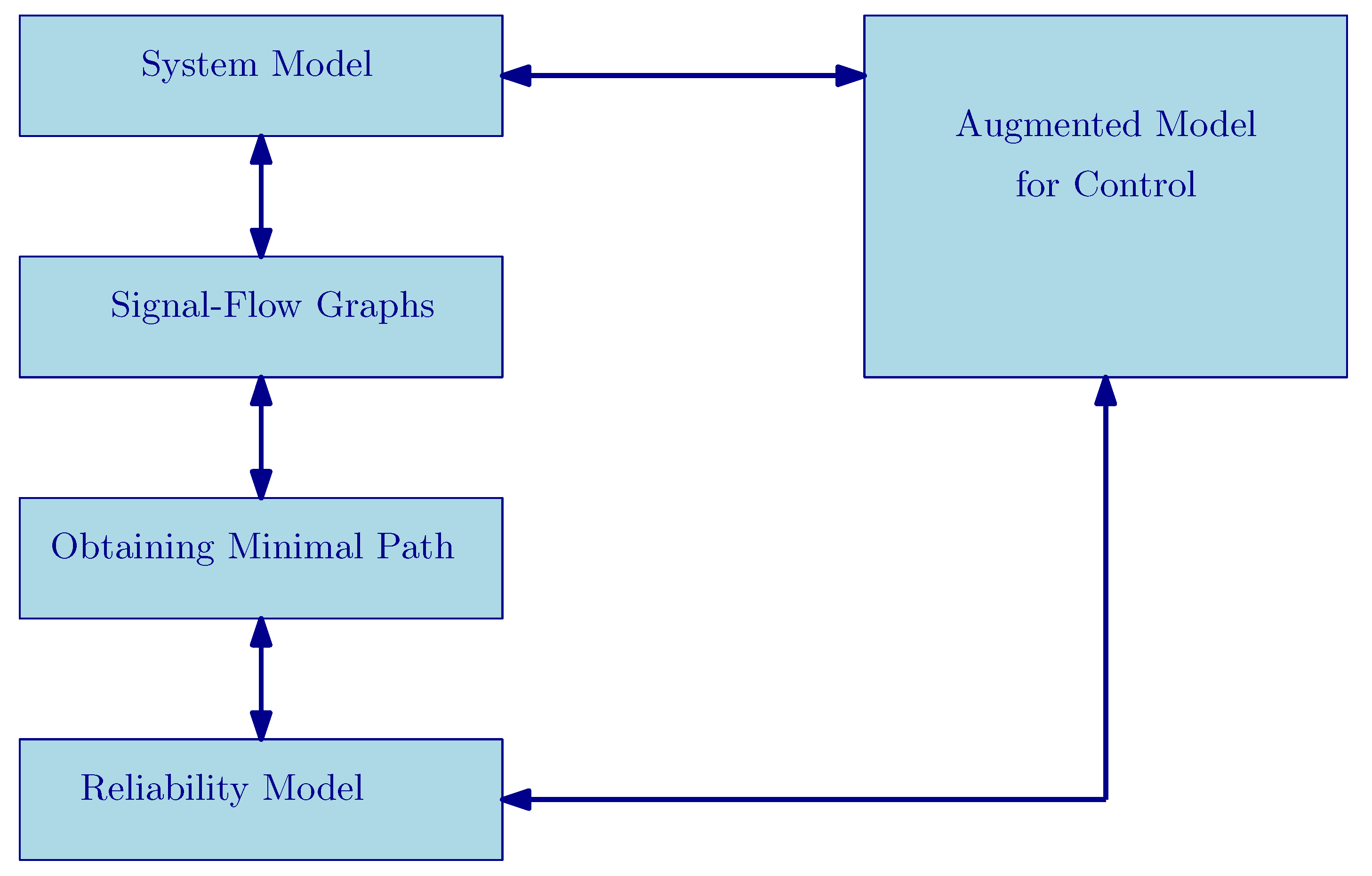
This section presents the incorporation of reliability information in the predictive control law as a new state of the model. As mentioned in Section 2, the reliability of the DWN can be estimated using the control input (actuator commands) information. To include a new objective in the MPC that proposes to extend the system reliability, the reliability model is represented by means of the model in Equation (22). In fact, the new control model of DWN that includes the reliability and dynamic model of DWN is obtained based on the structure shown in Figure 1. Actually, there is a direct relationship between the dynamic model of DWN and its system reliability.

Thus, the new MPC model has the following structure

$$\begin{array}{cc}{x}_r(k+1)& =A_r{x}_r(k)+B_{r}u(k)+B_{r,d}{d}_m(k),\hfill \\ y_r(k)& =C_{r}x(k),\hfill \end{array}$$

(23)

where the state and output vector are given by $x_r={[x,log(Q_G),log(R_1),\dots ,log(R_i)]}^T$ and $y_r={[y,log(Q_G)]}^T$, respectively. The new matrices are defined as

$$\begin{array}{cc}{A}_r& =\left[\begin{array}{ccc}A& & 0_{n_x\times n_{i+1}}\\ 0_{1\times n_x}& 1& {\displaystyle {\sum }_{i\in p_{s,j}}^s}{\beta }_j(k)\\ & & \\ 0_{n_i\times n_x}& & I_{n_i\times n_i}\\ & & \end{array}\right],B_r=\left[\begin{array}{c}{B}_{n_u\times n_u}\\ 0\\ & & \\ -{\lambda }_i\times I_{n_i\times n_i}\\ & & \end{array}\right],\hfill \\ B_{r,d}& =\left[\begin{array}{c}{B}_{d,n_u\times n_u}\\ & & \\ & & \\ 0_{n_{i+1}\times n_{B_d}}\\ & & \\ & & \end{array}\right],C_r=\left[\begin{array}{ccccc}C& 0& 0& \cdots & 0\\ 0& 1& 0& \cdots & 0\end{array}\right].\hfill \end{array}$$

(24)

Therefore, the new MPC model in Equation (23) can be viewed as an LPV model that has as scheduling variable the control action $u_i(k)$ related to each state and actuator. The new MPC model in Equation (23) cannot be estimated before solving the optimization problem in Equation (9) since the future state sequence is not identified. In fact, $x(l|k)$ depends on the future control inputs $u(k)$ and scheduling parameters, which, for general LPV models, are not expected to be known prior but only to be measurable online at current time k. The idea is to obtain a solution to the problem in Equation (9) by solving an online optimization problem as a QP problem. The solution for this problem is to modify the exact LPV-MPC to a linear approximation of the LPV-MPC. This approximation uses an estimation of scheduling variables, $\widehat{\theta }$, instead of applying $\theta$. Indeed, the scheduling variables in the prediction horizon are determined and used to update the matrices of the model adopted by the MPC controller. In fact, to solve this problem, the sequence of the control input is used to adjust the system matrices of the model applied in the prediction horizon. Hence, based on the optimal control sequence $\mathbf{u}$(k), the following sequence of states and predicted parameters can be achieved:

$$\tilde{\mathbf{x}}(k)=\left[\begin{array}{c}x(l+1|k)\\ x(l+2|k)\\ ⋮\\ x(N_p|k)\end{array}\right]\in {\mathbb{R}}^{N_p,n_x},\mathsf{\Theta }(k)=\left[\begin{array}{c}\widehat{\theta }(l|k)\\ \widehat{\theta }(l+1|k)\\ ⋮\\ \widehat{\theta }(N_p-1|k)\end{array}\right]\in {\mathbb{R}}^{N_p,n_{\theta }}.$$

(25)

Therefore, with slight abuse of notation, f can be defined as: $\mathsf{\Theta }(k)=f(\left[x^T(k){\tilde{\mathbf{x}}}^T(k)\right],u(k))$. The vector $\mathsf{\Theta }(k)$ includes parameters from time k to $k+N_p-1$ whilst the state prediction is accomplished for time $k+1$ to $k+N_p$.

Hence, by using the definitions in Equation (25), the predicted states can be simply formulated as follows

$$\tilde{\mathbf{x}}(k)=\mathcal{A}(\mathsf{\Theta }(k))x(k)+\mathcal{B}(\mathsf{\Theta }(k))u(k)+B_{r,d}{d}_m(k),$$

(26)

where $\mathcal{A}\in {\mathbb{R}}^{n_x\times n_x}$ and $\mathcal{B}\in {\mathbb{R}}^{n_x\times n_u}$ are given by Equations (27) and (28).

$$\mathcal{A}(\mathsf{\Theta }(k))=\left[\begin{array}{c}I\\ A(\widehat{\theta }(k))\\ A(\widehat{\theta }(k+1))A(\widehat{\theta }(k))\\ ⋮\\ A(\widehat{\theta }(k+N_p-1))A(\widehat{\theta }(k+N_p-2))\dots A(\widehat{\theta }(k))\end{array}\right],$$

(27)

and

$$\mathcal{B}(\mathsf{\Theta }(k))=\left[\begin{array}{ccccc}0& 0& 0& \dots & 0\\ B(\widehat{\theta }(k))& 0& 0& \dots & 0\\ A(\widehat{\theta }(k+1))B(\widehat{\theta }(k))& B(\widehat{\theta }(k+1))& 0& \dots & 0\\ ⋮& ⋮& \ddots & \ddots & ⋮\\ A({\widehat{\theta }}_{k+N_p-1})\dots A(\widehat{\theta }(k+1))B(\widehat{\theta }(k))& A({\widehat{\theta }}_{k+N_p-1})\dots A(\widehat{\theta }(k+2))B(\widehat{\theta }(k+1))& \dots & B({\widehat{\theta }}_{k+N_p-1}))& 0\end{array}\right].$$

(28)

By using Equation (26) and augmented block diagonal weighting matrices $\widetilde{w_1}=dia{g}_{N_p}(w_1)$ and $\widetilde{w_2}=dia{g}_{N_p}(w_2)$, the cost function in Equation (8) with new additional objective that aims to maximize the system reliability can be rewritten in vector form as

$$\begin{array}{c}\begin{array}{c}{\displaystyle {\displaystyle \underset{\mathbf{u}(k),\xi (k),log{Q}_G(k)}{min}}{\displaystyle \sum _{l=0}^{N_p}}[{\ell }_e(l|k)+{\ell }_s(l|k)+{\ell }_{\Delta u}(l|k)-{\ell }_{Rg}(l|k)],}\end{array}\end{array}$$

(29a)

subject to:

$$\begin{array}{c}\tilde{\mathbf{x}}(k)=\mathcal{A}(\mathsf{\Theta }(k))x(k)+B_{r,d}{d}_m(k),\mathcal{B}(\mathsf{\Theta }(k))u(k),\hfill \end{array}$$

(29b)

$$\begin{array}{c}0=E_{u}u(l|k)+E_d{d}_m(k),\hfill \end{array}$$

(29c)

$$\begin{array}{c}x(l+1|k)\ge x_s-\xi (l|k)\hfill \end{array}$$

(29d)

$$\begin{array}{c}log{Q}_G(l+1|k)={\tilde{\mathbf{x}}}_{nx+1}(l|k)\hfill \end{array}$$

(29e)

$$\begin{array}{c}u(l|k)\in \mathbb{U},l=0,\cdots ,N_p-1\hfill \end{array}$$

(29f)

$$\begin{array}{c}x(l|k),\in \mathbb{X},l=1,\cdots ,N_p\hfill \end{array}$$

(29g)

$$\begin{array}{c}\xi (l|k)\ge 0,l=0,\cdots ,N_p\hfill \end{array}$$

(29h)

$$\begin{array}{c}x(0|k)=x(k),\hfill \end{array}$$

(29i)

where ${\ell }_{Rg}(k)\triangleq log{Q}_G^{\mathsf{\top }}{w}_{3}log{Q}_G$ is additional objective with the corresponding weight $w_3$ into the EMPC-LPV cost function to maximize the system reliability. Since the predicted states $\mathsf{\Theta }(k)$ in Equation (26) are linear in control inputs $u(k)$, the optimization problem can be solved as a QP problem, which is significantly easier than solving a nonlinear optimization problem.

Using this idea, the following iterative approach at each time instant k is applied:

• In the first iteration, the problem in Equation (9) is solved considering that the quasi-LPV model in Equation (23) is instantiated by the LTI model considering that $\theta (0|l)$≃$\theta (1|l)$≃$\theta (2|l)$≃… ≃$\theta (N_p-1|l)$ along the prediction horizon $N_p$.
• The parameter varying sequence $\mathsf{\Theta }(k)$ is updated using the optimal value of the scheduling variables ${\mathsf{\Theta }}^{*}(k)=f({\tilde{\mathbf{x}}}^{*}(k),{\mathbf{u}}^{*}(k))$, where ${\tilde{\mathbf{x}}}^{*}(k)$ and ${\mathbf{u}}^{*}(k)$ are the optimal input and state sequences obtained after the solution of the MPC problem, respectively.
• The parameter varying values for the next iteration $\mathsf{\Theta }(k+1)$ are obtained considering $\tilde{\mathbf{x}}(k)$ and $\tilde{u}(k)$, i.e., ${\mathsf{\Theta }}_0(k+1)=f({\tilde{\mathbf{x}}}_1(k),{\mathbf{u}}_0(k))$.

5. Application to the Water Transport Network of Barcelona

In this section, two motivational examples are used to assess the implementation of the proposed economic health-aware LPV-MPC based on system reliability assessment. For both examples, the system under study is a portion extracted from the Barcelona DWN [34]. This network is managed by Aguas de Barcelona (AGBAR), which supplies drinking water for Barcelona and its metropolitan area [35]. The general task of this system is to supply water resources from sources to consumers minimizing the operational costs. The DWN of Barcelona covers a territorial extension of 425 km${}^2$, with a total pipe length of 4470 km. Every year, it supplies $237.7$ hm${}^3$ of drinking water to a population over $2.8$ million inhabitants. Regarding the DWN reliability study, sectors, sources, pipelines and tanks are assumed to be perfectly reliable, whereas active elements such as pumps and valves are considered not completely reliable [4]. The results were obtained using a 2.4 GHz and 12.00 Gb RAM Intel(R) Core(TM)i7-5500 CPU. Matlab and Yalmip toolbox were used to perform the simulations.

5.1. Water Transport Network (3-Tanks)

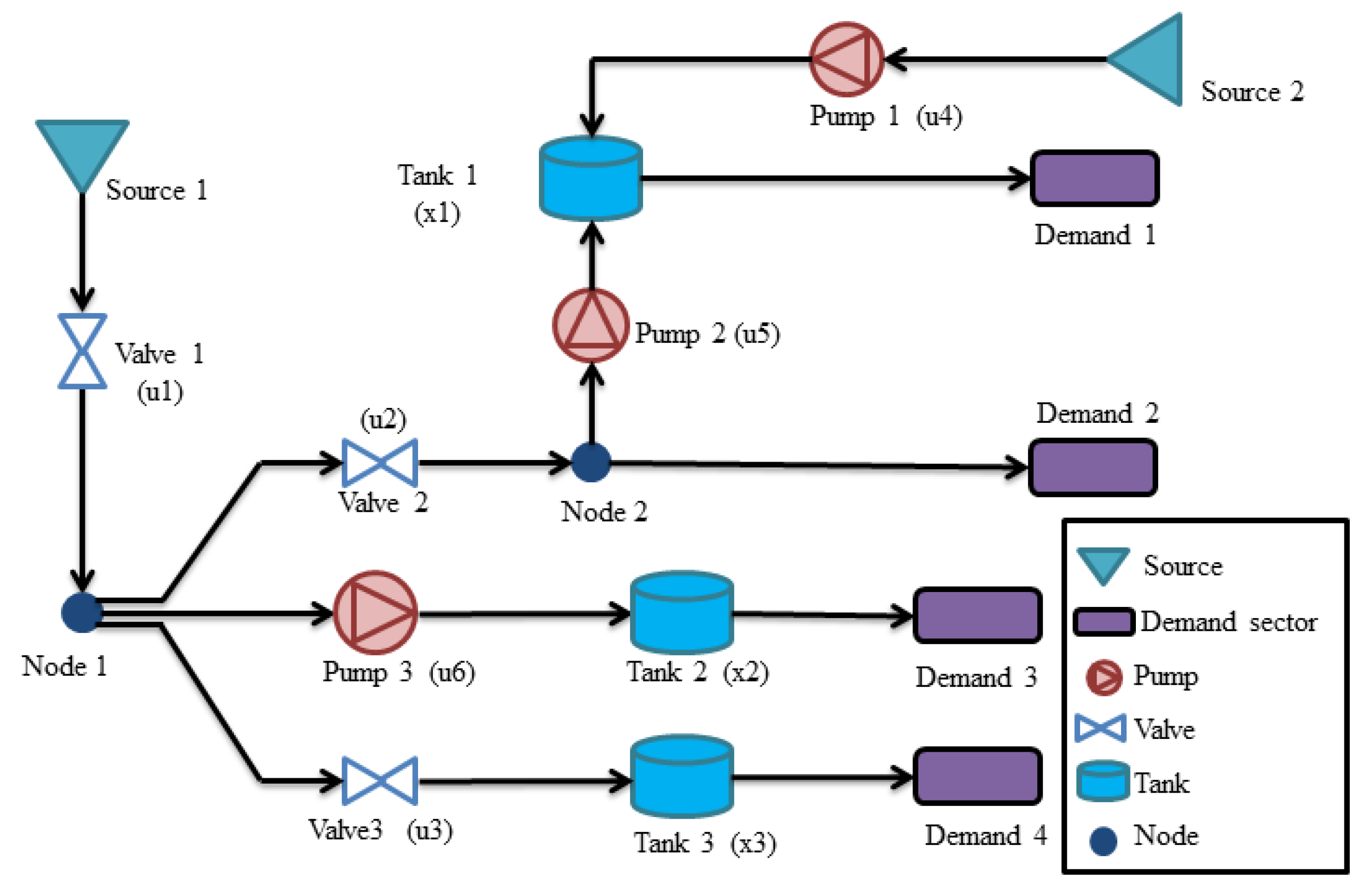
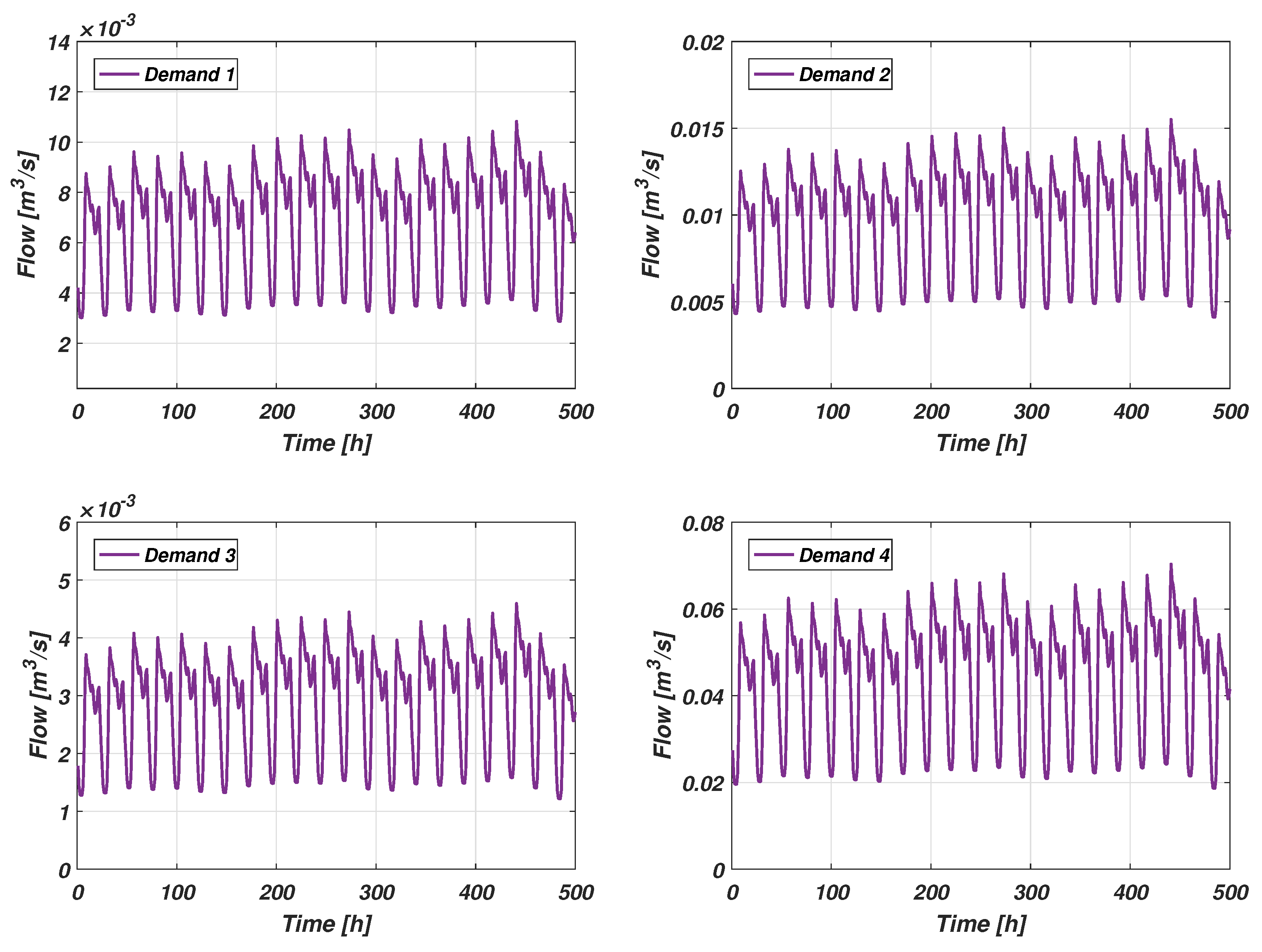
In the first example, the proposed study concentrates on a small network based on the Barcelona DWN. Two sources of water and four demand sectors, which represent the district metered area (DMA), are considered (see Figure 2). It is expected that the demand forecast ($d_m$) at each demand sector is known and that every single source can provide this water demand (Figure 3). First, system components must be identified. In this case, there are three pumps, three valves, two sources, three tanks, two intersection nodes, and several pipes.

Afterwards, according the definition of minimal path $P_s$ in Section 3.2, the minimal path sets is determined for the water network, while the $P_s$ is determined based on the relation and the possible connection between each source and demand sector. By considering all the paths from all sources to the demand sector, the combination of all flow paths should follow the functional requirements necessary to satisfy the consumer demands. A minimal path set is composed by those elements which allow a flow path between sources and demand sector, such as pipes, tanks, pumps and valves. Based on this analysis, the following list of each minimal path is presented in

Table 1. Success minimal paths of the water transport network of Barcelona (three tanks).

Path	Component Set
$P_1$	$\left\{Source1,Valve1,Valve3,Demand4\right\}$
$P_2$	$\left\{Source1,Valve1,Pump2,Demand3\right\}$
$P_3$	$\left\{Source1,Valve1,Valve2,Demand2\right\}$
$P_4$	$\left\{Source1,Valve1,Valve2,Pump2,Demand1\right\}$
$P_5$	$\left\{Source2,Pump1,Demand1\right\}$

. There are five minimal path sets in the system of Figure 2. The reliability of each minimal path set depends on the reliability of its components. Tanks and pipes are supposed to be perfectly reliable. However, sources are involved in the minimal path sets only for illustrative purposes of the proposed procedure.

Table 2. Simulation parameters.

Parameter	Value
$Np$	24
$T_s$ [h]	1
$T_m$ [h]	200
${\alpha }_1$	0.123    0    0    0.054    0    0
$u_{min}$ [m${}^3$/s]	0    0    0    0    0    0
$u_{max}$ [m${}^3$/s]	1.297    0.05    0.12    0.015    0.0317    0.022
${\lambda }_0$ [h${}^{-1}\times$ h${}^{-4}$]	1.2   3.45    6.3    9.5    1    1
$x_{min}$ [m${}^3$]	0    0    0    0    0    0    0    0    0    0
$x_{max}$ [m${}^3$]	470  960  3100   1    1    1    1    1    1    1
$x_0$ [m${}^3$]	0.75    0.62    0.34    0    1    1    1    1    1    1

provides the simulation parameters used.

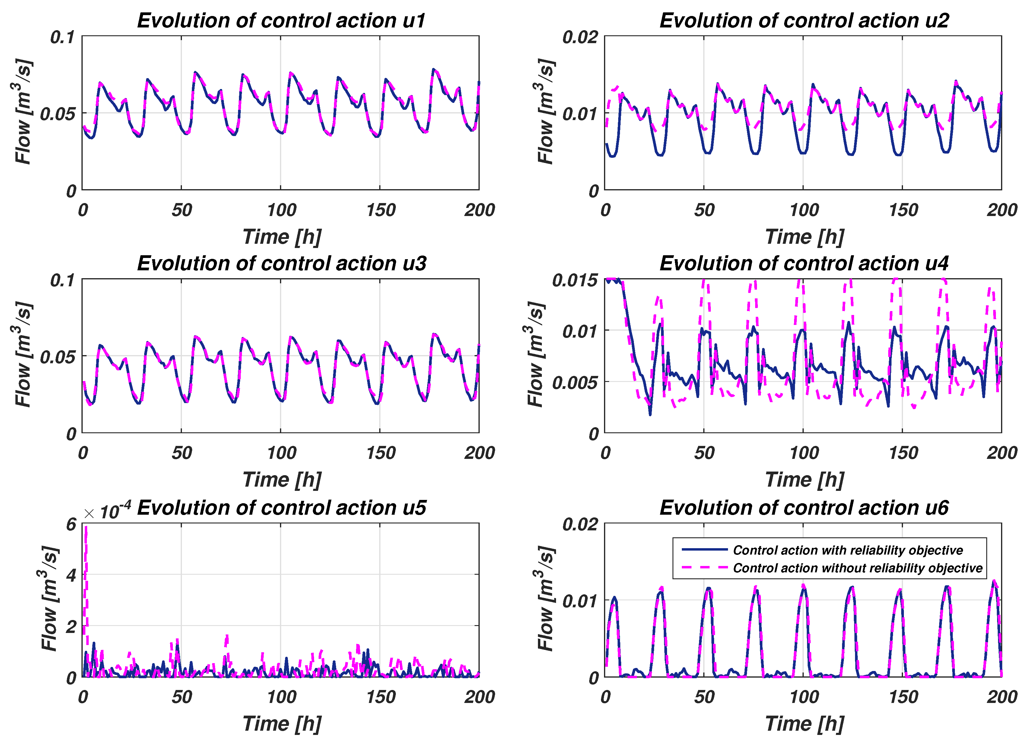
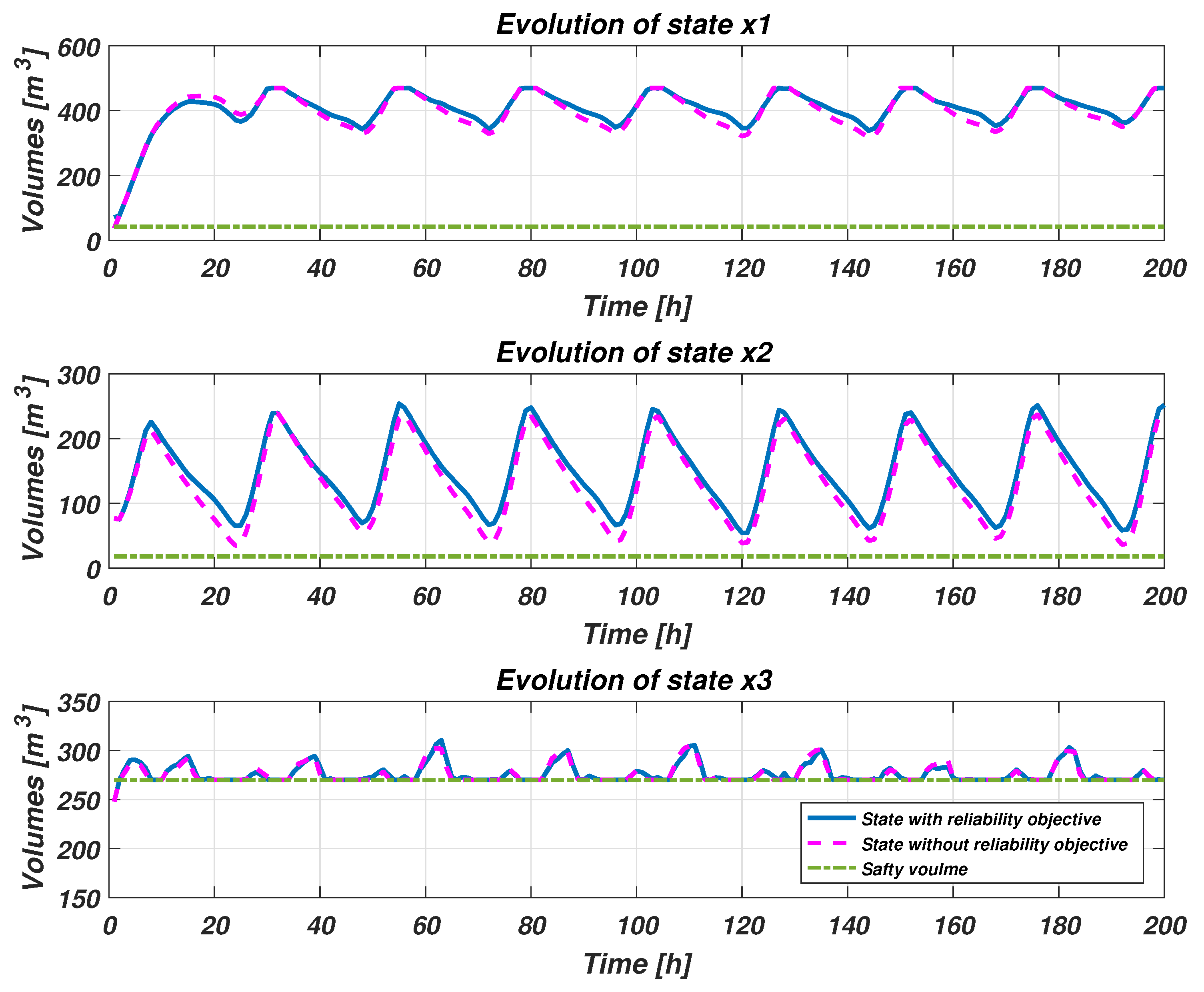
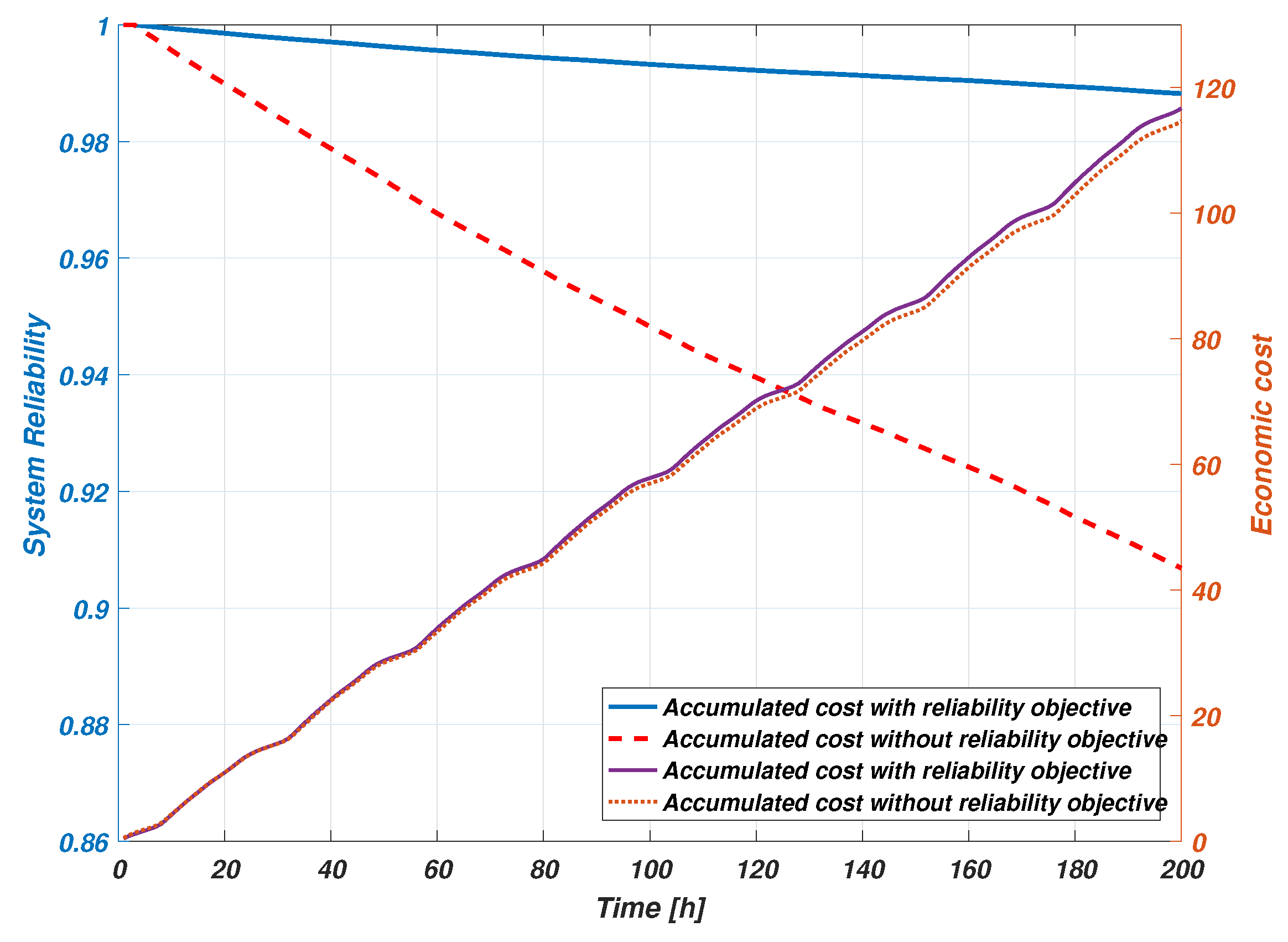
Figure 4 shows the evolution of the valves and pumps commands that were obtained using the new approach of the health-aware LPV-MPC in the three tanks example with and without the reliability-aware objective. As can be seen in Figure 4, the behavior of valve control actions are different from the ones corresponding to the pumps. However, in all of them, the behaviors of control actions in both scenarios are almost the same, thus the reliability-aware objective is not significantly affecting the behavior of the valves and pumps. The comparison of the volume evolution of three tanks based on the health-aware LPV-MPC with and without the reliability-aware objective is presented in Figure 5. The safety volume of each tank is satisfied and hence able to cope with unexpected demands. The system reliability prediction of the DWN, which was obtained when using the proposed controller with and without the reliability-aware objective, is presented in Figure 6. According to these results, it can be observed that, with the use of reliability-aware objective in the MPC, the network reliability is better preserved compared to the case that the reliability is not considered in the MPC objectives. However, the responses of water tanks are similar in both scenarios. The trade-off between the decreasing operating cost and increasing system reliability can be observed in Figure 6. Note that the differences in the amount of the operational cost using the proposed approach is similar to the EMPC controller without reliability objective. Figure 6 shows that the system reliability is increased from $0.9071$ to $0.9891$ and that is about $9.06\%$ of improvement, while the accumulated cost is increased from $114.6$ to $116.7$ that is about $1.74\%$ of increment.

5.2. Water Transport Network of Barcelona (17-Tanks)

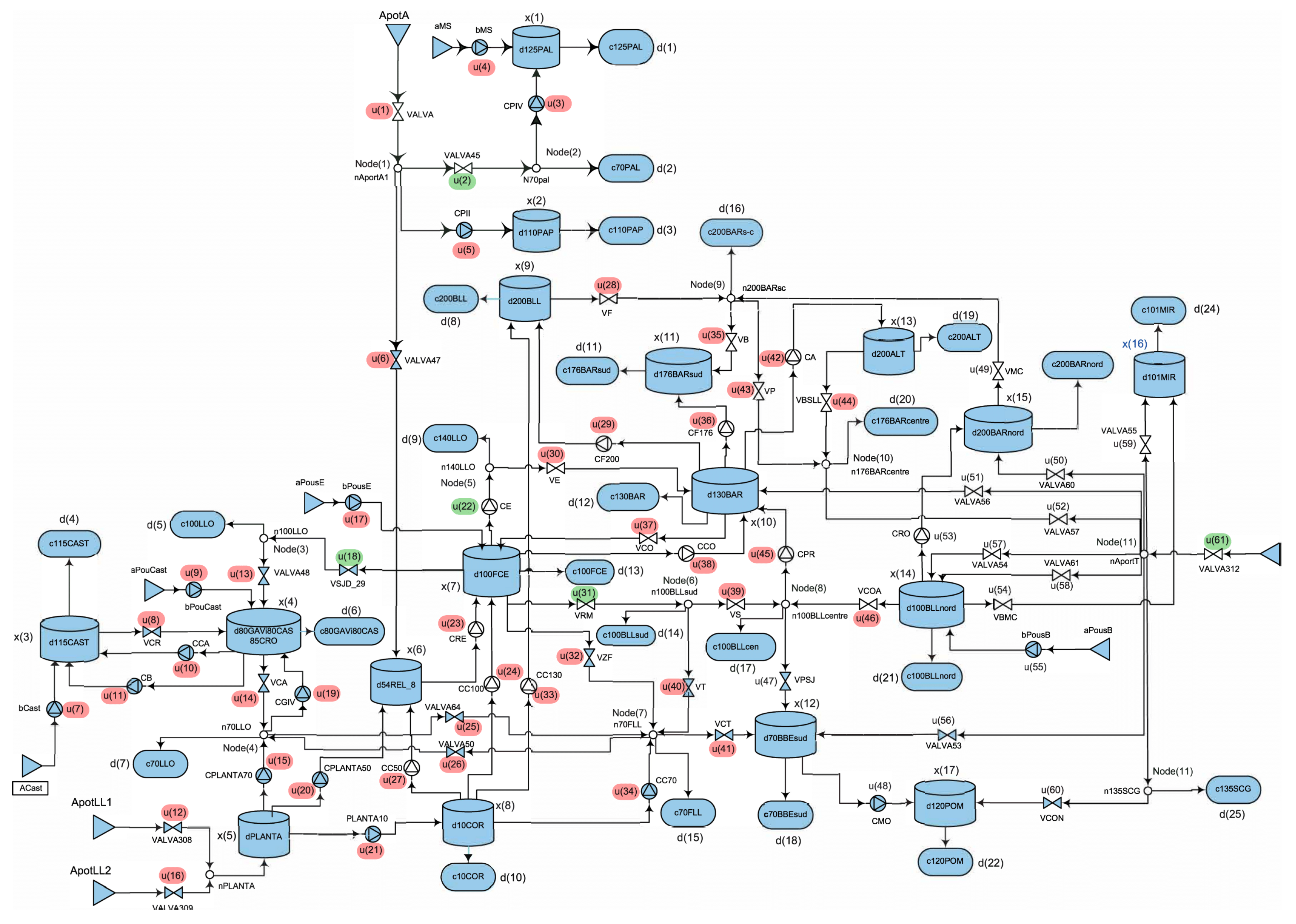
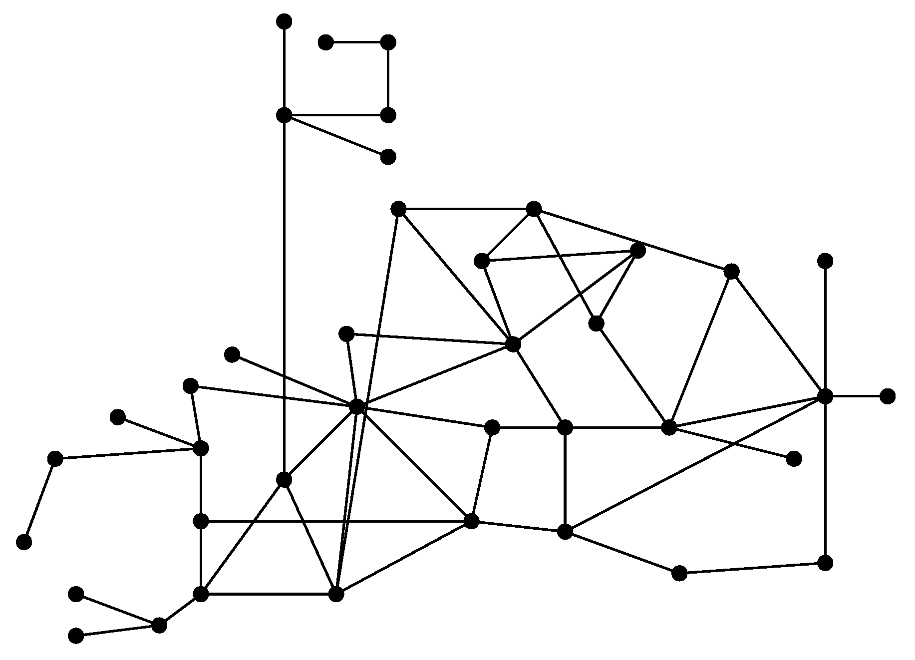
Now, a more complex and realistic example also based on the Barcelona DWN is considered as a case study. This case includes 17 tanks and nine sources, consisting of five underground and four surface sources, which currently provide an inflow of about 2 m${}^3$/s. The case study also includes 61 actuators (valves and pumps), 12 nodes and 25 demands. Figure 7 presents the general topology of the network, showing a complex system in terms of its elements and the relationships and connections between them. Figure 8 presents the graph obtained from this network; the nodes correspond to reservoirs or pipe merging/splitting nodes and the arcs correspond to actuators (pumps and valves). The graph of the water network was obtained from the state space representation of the system. This approach is explained with more detail in [36].

As in the previous example, demand sectors, sources, pipelines and tanks are considered perfectly reliable, whereas actuators are not [4]. Moreover, it is expected that the demand forecast ($d_m$) at each demand sectors is known and that every single source can supply the required water demand (see some demand sectors in Figure 9).

The economic reliability-aware LPV-MPC formulation proposed in previous section was applied to the simulation model of the DWN presented in Figure 9.

From the reliability analysis, it could be obtained which states are structurally controllable since the path computation analysis provide all possible paths from a source to a target sectors. Moreover, for each path, an approximate operational cost (according to the electricity cost of each element) and a maximal water flow (according to the physical constraints of the actuators) can also be derived.

Table 3. Structural actuators (towards tanks).

No.	Name	No.	Name	No.	Name	No.	Name
$u_1$	VALVA	$u_{16}$	VALVA309	$u_{33}$	CC130	$u_{47}$	VPSJ
$u_3$	CPIV	$u_{17}$	bPousE	$u_{34}$	CC70	$u_{48}$	CMO
$u_4$	bMS	$u_{19}$	CGIV	$u_{35}$	VB	$u_{49}$	VMC
$u_5$	CPII	$u_{20}$	CPLANTA50	$u_{36}$	CF176	$u_{50}$	VALVA60
$u_6$	VALVA47	$u_{21}$	PLANTA10	$u_{37}$	VCO	$u_{51}$	VALVA56
$u_7$	bCast	$u_{23}$	CRE	$u_{38}$	CCO	$u_{52}$	VALVA57
$u_8$	VCR	$u_{24}$	CC100	$u_{39}$	VS	$u_{53}$	CRO
$u_9$	bPouCast	$u_{25}$	VALVA64	$u_{40}$	V	$u_{54}$	VBMC
$u_{10}$	CCA	$u_{26}$	VALVA50	$u_{41}$	VCT	$u_{55}$	bPousB
$u_{11}$	CB	$u_{27}$	CC50	$u_{42}$	CA	$u_{56}$	VALVA53
$u_{12}$	VALVA308	$u_{28}$	VF	$u_{43}$	VP	$u_{57}$	VALVA54
$u_{13}$	VALVA48	$u_{29}$	CF200	$u_{44}$	VBSLL	$u_{58}$	VALVA61
$u_{14}$	VCA	$u_{30}$	VE	$u_{45}$	CPR	$u_{59}$	VALVA55
$u_{15}$	CPLANTA70	$u_{32}$	VZF	$u_{46}$	VCOA	$u_{60}$	VCON

and

Table 4. Structural actuators (towards demand nodes).

No.	Name	No.	Name	No.	Name	No.	Name
$u_2$	VALVA45	$u_{18}$	VSJD-29	$u_{22}$	CE	$u_{31}$	VRM
$u_{61}$	VALVA312

show that there exist several critical actuators within the network, considering the topology and the way of network elements are connected, as most actuators (valves or pumps) are the only link between demands and tanks. Consequently, if an actuator fails, then the corresponding demand will not be satisfied. Therefore, if an actuator fails, then the corresponding demand will not be satisfied. Note that the information shown in Table 3 and Table 4 is especially significant for AGBAR since it identifies the critical elements in the network for surveillance/correction policies to be implemented in the event of element damage [5]. According to the DWN (Figure 7), Table 3 and Table 4 and the above analysis of the success minimal path of the water network, there are 607 minimal path sets in the system of Figure 7. Some samples of success minimal paths are presented in

Table 5. Some success minimal paths of the Barcelona DWN.

Path	Component Set
$P_1$	$\left\{aMS,bMS,c125PAL\right\}$
$P_2$	$\left\{AportA,VALVA,VALVA47,CPIV,c125PAL\right\}$
$P_3$	$\left\{AportA,VALVA,VALVA45,c70PAL\right\}$
$P_4$	$\left\{AportA,VALVA,CPII,c110PAP\right\}$
$P_5$	$\left\{ACast,bCast,c115CAST\right\}$
⋮	⋮
$P_{607}$	$\left\{AportT,VALVA312,c135SCG\right\}$

. The objective of the MPC as explained above is to minimize the multi-objective cost function in Equation (29). The prediction horizon is 24 h because the system and the electrical tariff have periodicity of one day. The sampling time is 1 h. However, in all of them, the behaviors of control actions in both scenarios are almost the same, considering the reliability-aware objective doe not greatly affect the behavior of the valves and pumps.

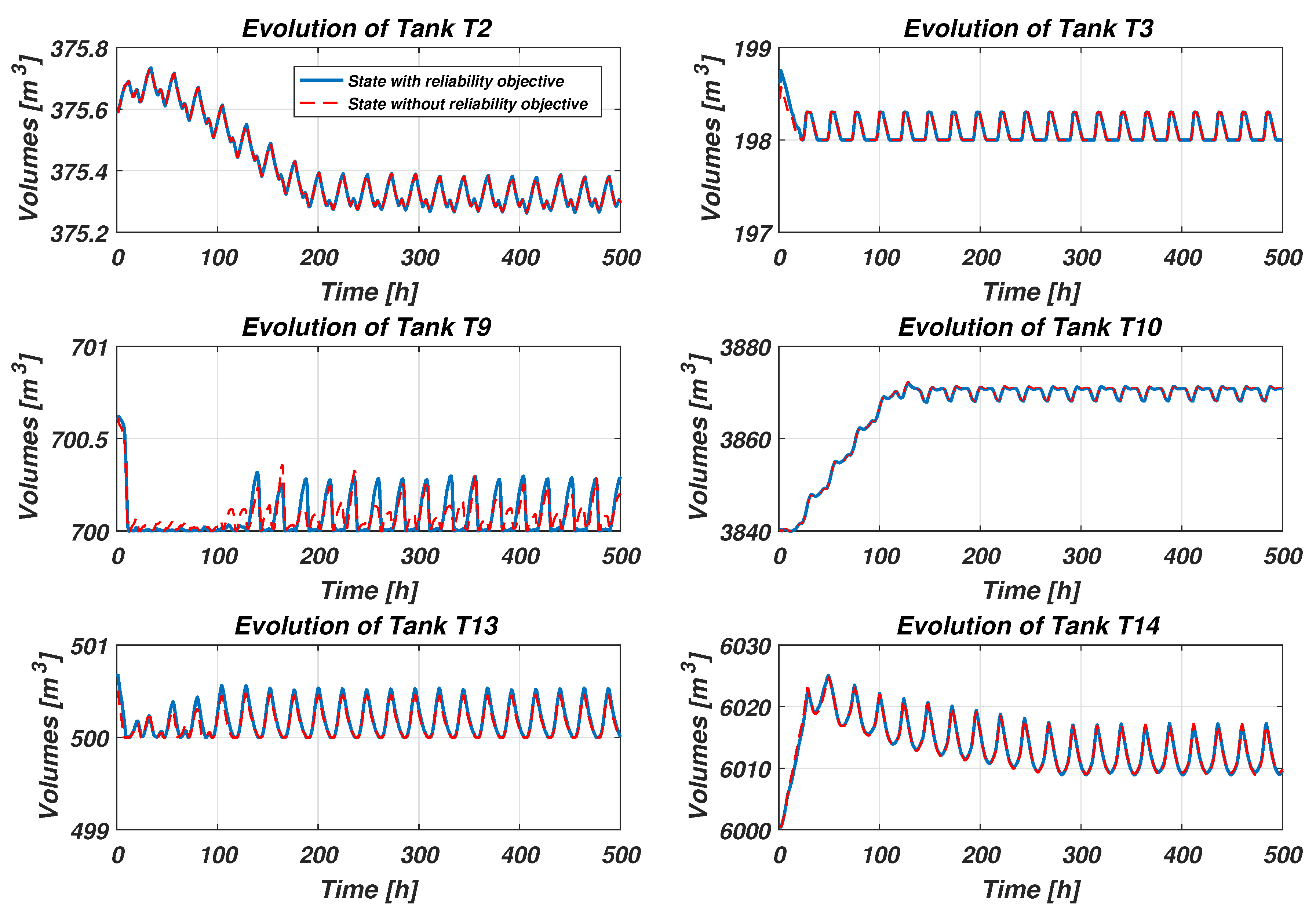
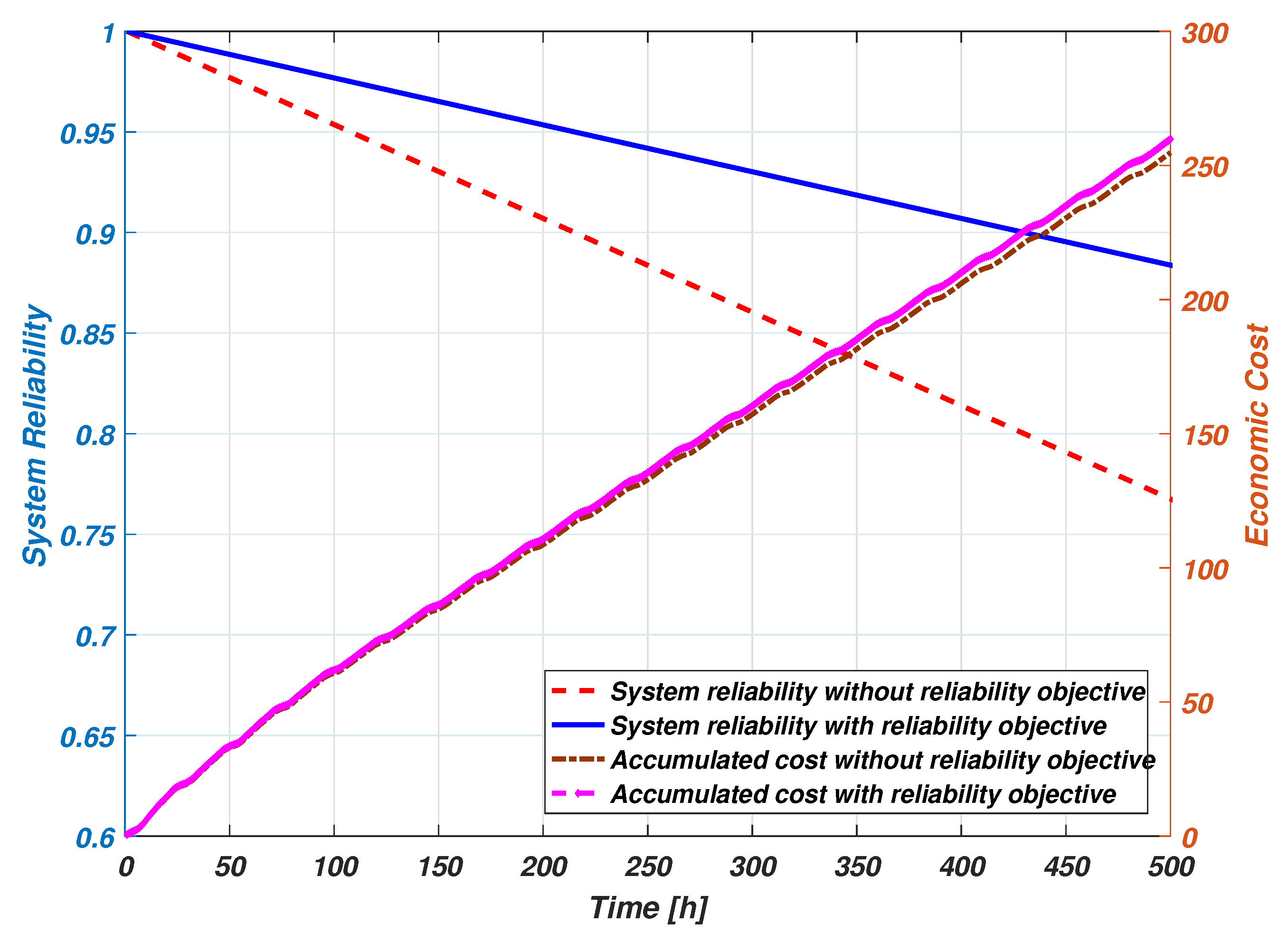
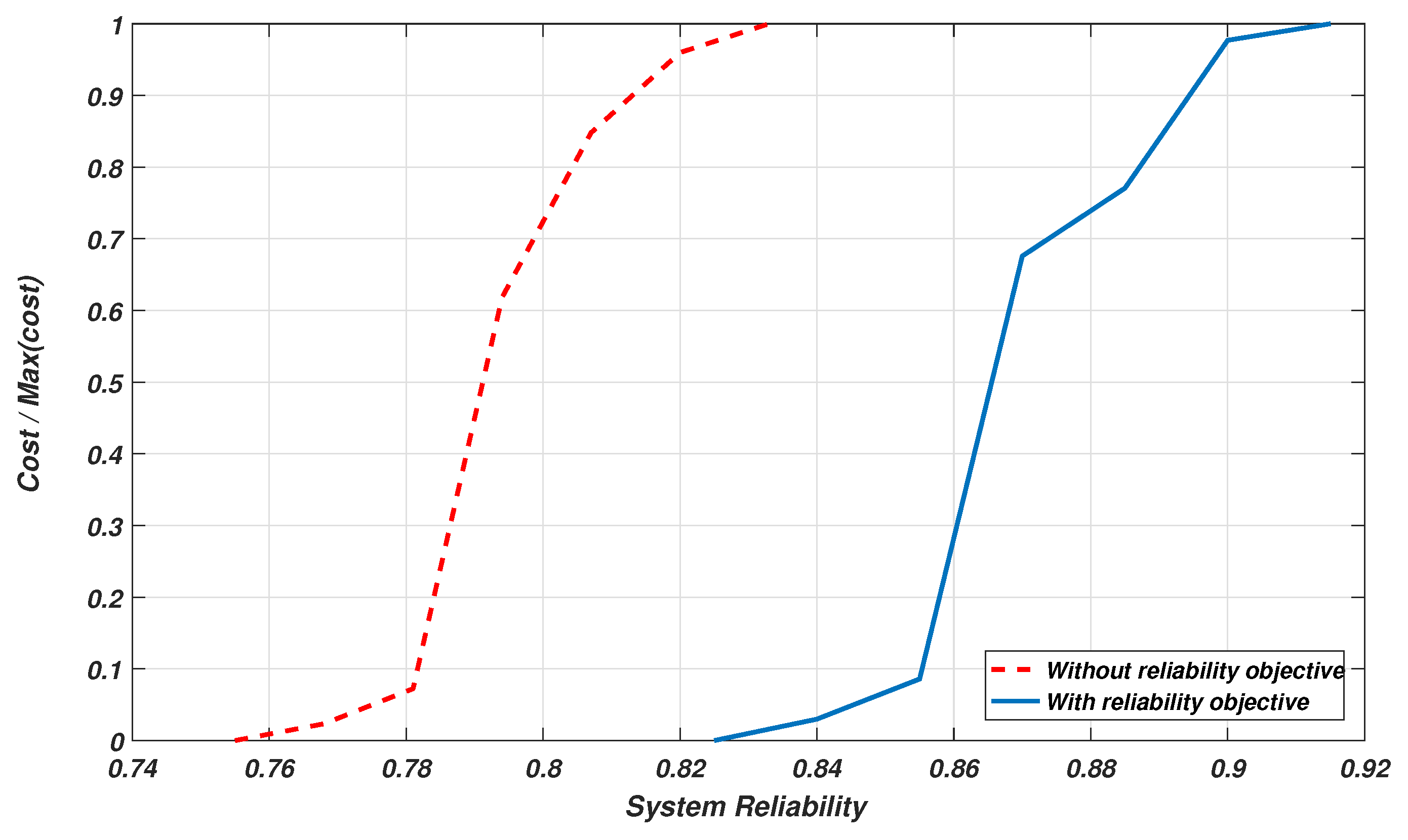
Figure 10 shows the comparative evolution of the valves and pumps commands obtained using the new approach with the case without the reliability-aware objective. Note that the plot of control actions 5, 7, 42, and 29 correspond to pump set-points while control actions 51 and 52 correspond to valve set-points (see Figure 7). The behavior of pumps and valves in both scenarios are almost the same even by including the reliability objective inside the cost function of the controller. Figure 11 presents the comparison of volume evolutions of selected storage tanks. Figure 11 shows the proper replenishment planning that the predictive controller dictates according to the cyclic behavior of demands. Notice that the net demand of each tank is properly satisfied along the simulation horizon. The system reliability evolution of the DWN that was obtained from the proposed controller with and without the reliability-aware objective is presented in Figure 12. According to these results, it can be observed that, with the use of reliability-aware objective in the MPC, the reliability of the network is better preserved compared to the case that the reliability is not considered in the MPC design. There is a trade-off between the increasing system reliability and operational cost. However, the operational cost obtained with new proposed approach is almost the same as the EMPC controller that not considers reliability. This figure also shows that the system reliability is improved about $14.73\%$ in the case of the LPV-MPC controller with the reliability objective while keeping the performance and the cost is increased just $2.03\%$. To have better compare the economics of LPV-MPC with and without the reliability-aware objective, several simulations with different tunings were implemented. Finally, the trade-off curves between the system reliability and economic operational cost for both control schemes are presented in Figure 13. This figure shows that independently of the tuning the economic reliability-aware LPV-MPC control is able to improve and increase the system reliability. The results obtained from the preliminary analysis of Figure 13 are provided in

Table 6. Final system reliability.

Different Weight Tuning Points	1	2	3	4	5	6	7
Economic LPV-MPC with reliability-aware objective	0.825	0.84	0.855	0.87	0.885	0.9	0.915
Economic LPV-MPC without reliability-aware objective	0.755	0.768	0.781	0.794	0.805	0.82	0.833
Difference percentage %	9.27	9.38	9.48	9.57	9.94	9.76	9.84

and

Table 7. Economic cost.

Different Weight Tuning Points	1	2	3	4	5	6	7
Economic LPV-MPC with reliability-aware objective	252.05	252.1	252.23	253.82	254.08	254.63	254.78
Economic LPV-MPC without reliability-aware objective	252.00	252.06	252.14	253.66	254.28	254.58	254.69
Difference percentage %	0.02	0.02	0.04	0.08	0.16	0.02	0.04

. The results, as shown in these tables, indicate that the system reliability is improved in different tunings while the cost is increased. However, the increased percentage of operational cost is negligible compared to the improvement of reliability obtained.

6. Conclusions

This paper proposes an economic health-aware LPV-MPC strategy based on the system reliability for water transport networks.

The system reliability is evaluated online considering the control action value. The system reliability is obtained from the reliability of each component and the interconnection topology leading to a nonlinear model. This model is transformed into a linear-like form by means of the LPV framework.

The system reliability is considered during the calculation of the MPC control action by including an extra objective in the cost function and an by augmenting the MPC model with additional states. Then, the by using a LPV-MPC approach, the associated optimization problem can be efficiently solved using quadratic programming. The MPC model is updated at each time iteration instantiating the varying parameters considering the value of the scheduling variables.

The results show that, using the proposed economic health-aware LPV-MPC, the DWN network reliability is maximized with a slight rise in the cost, achieving a good trade-off between both system reliability and cost. In this way, it is possible to maximize the lifetime of elements just by reducing slightly the economic optimality.

Future research will extend the study to water distribution networks by considering the pressure model. Moreover, the problem of re-designing the network by adding some additional paths to overcome the limitations due to critical elements. Moreover, it would be interesting to consider the water quality objective into the proposed approach.

References

- Ocampo-Martinez, C.; Puig, V.; Cembrano, G.; Quevedo, J. Application of predictive control strategies to the management of complex networks in the urban water cycle [applications of control]. IEEE Control Syst. 2013, 33, 15–41. [Google Scholar]
- Barbieri, M.; Nigro, A.; Petitta, M. Groundwater mixing in the discharge area of San Vittorino Plain (Central Italy): Geochemical characterization and implication for drinking uses. Environ. Earth Sci. 2017, 76, 393. [Google Scholar] [CrossRef]
- Grosso, J.M.; Ocampo-Martínez, C.; Puig, V. A service reliability model predictive control with dynamic safety stocks and actuators health monitoring for drinking water networks. In Proceedings of the 2012 IEEE 51st Annual Conference on Decision and Control (CDC), Maui, HI, USA, 10–13 December 2012; pp. 4568–4573. [Google Scholar]
- Weber, P.; Simon, C.; Theilliol, D.; Puig, V. Fault-Tolerant Control Design for over-actuated System conditioned by Reliability: A Drinking Water Network Application. IFAC Proc. Vol. 2012, 45, 558–563. [Google Scholar] [CrossRef]
- Robles, D.; Puig, V.; Ocampo-Martinez, C.; Garza-Castañón, L.E. Reliable fault-tolerant model predictive control of drinking water transport networks. Control. Eng. Pract. 2016, 55, 197–211. [Google Scholar] [CrossRef] [Green Version]
- Karimi Pour, F.; Puig, V.; Ocampo-Martinez, C. Health-aware Model Predictive Control of Pasteurization Plant. In Journal of Physics: Conference Series; IOP Publishing: Bristol, UK, 2017; Volume 783, p. 012030. [Google Scholar]
- Ocampo-Martinez, C.; Ingimundarson, A.; Puig, V.; Quevedo, J. Objective prioritization using lexicographic minimizers for MPC of sewer networks. IEEE Trans. Control. Syst. Technol. 2008, 16, 113–121. [Google Scholar] [CrossRef]
- Pascual, J.; Romera, J.; Puig, V.; Cembrano, G.; Creus, R.; Minoves, M. Operational predictive optimal control of Barcelona water transport network. Control. Eng. Pract. 2013, 21, 1020–1034. [Google Scholar] [CrossRef] [Green Version]
- Rawlings, J.B.; Mayne, D.Q. Model Predictive Control: Theory and Design; Nob Hill Pub: San Francisco, CA, USA, 2009. [Google Scholar]
- Ellis, M.; Durand, H.; Christofides, P.D. A tutorial review of economic model predictive control methods. J. Process Control. 2014, 24, 1156–1178. [Google Scholar] [CrossRef]
- Karimi Pour, F.; Puig, V.; Ocampo-Martinez, C. Economic Predictive Control of a Pasteurization Plant using a Linear Parameter Varying Model. In Computer Aided Chemical Engineering; Elsevier: Amsterdam, The Netherlands, 2017; Volume 40, pp. 1573–1578. [Google Scholar]
- Karimi Pour, F.; Puig, V.; Cembrano, G. Health-aware LPV-MPC Based on System Reliability Assessment for Drinking Water Networks. In Proceedings of the 2018 IEEE Conference on Control Technology and Applications (CCTA), Copenhagen, Denmark, 21–24 August 2018; pp. 187–192. [Google Scholar]
- Edwards, M. Critical Infrastructure Protection; IOS Press: Amsterdam, The Netherlands, 2014; Volume 116. [Google Scholar]
- Chamseddine, A.; Theilliol, D.; Sadeghzadeh, I.; Zhang, Y.; Weber, P. Optimal reliability design for over-actuated systems based on the MIT rule: Application to an octocopter helicopter testbed. Reliab. Eng. Syst. Saf. 2014, 132, 196–206. [Google Scholar] [CrossRef]
- Gokdere, L.; Chiu, S.L.; Keller, K.J.; Vian, J. Lifetime control of electromechanical actuators. In Proceedings of the 2005 IEEE Aerospace Conference, Big Sky, MT, USA, 5–12 March 2005; pp. 3523–3531. [Google Scholar]
- Li, Y.; Kurfess, T.; Liang, S. Stochastic prognostics for rolling element bearings. Mech. Syst. Signal Process. 2000, 14, 747–762. [Google Scholar] [CrossRef]
- Salazar, J.C.; Weber, P.; Sarrate, R.; Theilliol, D.; Nejjari, F. MPC design based on a DBN reliability model: Application to drinking water networks. IFAC-PapersOnLine 2015, 48, 688–693. [Google Scholar] [CrossRef] [Green Version]
- Pereira, E.B.; Galvão, R.K.H.; Yoneyama, T. Model predictive control using prognosis and health monitoring of actuators. In Proceedings of the 2010 IEEE International Symposium on Industrial Electronics (ISIE), Bari, Italy, 4–7 July 2010; pp. 237–243. [Google Scholar]
- Karimi Pour, F.; Puig, V.; Cembrano, G. Health-aware LPV-MPC based on a Reliability-based Remaining Useful Life Assessment. IFAC-PapersOnLine 2018, 51, 1285–1291. [Google Scholar] [CrossRef]
- Farmani, R.; Walters, G.; Savic, D. Evolutionary multi-objective optimization of the design and operation of water distribution network: total cost vs. reliability vs. water quality. J. HydroInform. 2006, 8, 165–179. [Google Scholar] [CrossRef]
- Ostfeld, A. Reliability analysis of water distribution systems. J. Hydroinform. 2004, 6, 281–294. [Google Scholar] [CrossRef] [Green Version]
- Christodoulou, S.E. Water network assessment and reliability analysis by use of survival analysis. Water Resour. Manag. 2011, 25, 1229–1238. [Google Scholar] [CrossRef]
- Beal, L.D.; Petersen, D.; Pila, G.; Davis, B.; Warnick, S.; Hedengren, J.D. Economic Benefit from Progressive Integration of Scheduling and Control for Continuous Chemical Processes. Processes 2017, 5, 84. [Google Scholar] [CrossRef]
- Kunz, K.; Huck, S.M.; Summers, T.H. Fast model predictive control of miniature helicopters. In Proceedings of the 2013 European Control Conference (ECC), Zurich, Switzerland, 17–19 July 2013; pp. 1377–1382. [Google Scholar]
- Bumroongsri, P.; Kheawhom, S. MPC for LPV systems based on parameter-dependent Lyapunov function with perturbation on control input strategy. Eng. J. 2012, 16, 61. [Google Scholar] [CrossRef]
- Karimi Pour, F.; Puig Cayuela, V.; Ocampo-Martínez, C. Comparative assessment of LPV-based predictive control strategies for a pasteurization plant. In Proceedings of the 4th-2017 International Conference on Control, Decision and Information Technologies, Barcelona, Spain, 5–7 April 2017; pp. 1–6. [Google Scholar]
- Cembrano, G.; Quevedo, J.; Salamero, M.; Puig, V.; Figueras, J.; Martı, J. Optimal control of urban drainage systems. A case study. Control. Eng. Pract. 2004, 12, 1–9. [Google Scholar] [CrossRef]
- Mays, L. Urban Stormwater Management Tools; McGraw Hill Professional: New York, NY, USA, 2004. [Google Scholar]
- Brdys, M.; Ulanicki, B. Operational Control of Water Systems: Structures, Algorithms and Applications. Automatica 1996, 32, 1619–1620. [Google Scholar]
- Maciejowski, J.M. Predictive Control: With Constraints; Pearson Education: London, UK, 2002. [Google Scholar]
- Gertsbakh, I. Reliability Theory: With Applications to Preventive Maintenance; Springer: London, UK, 2013. [Google Scholar]
- Jiang, R.; Jardine, A.K. Health state evaluation of an item: A general framework and graphical representation. Reliab. Eng. Syst. Saf. 2008, 93, 89–99. [Google Scholar] [CrossRef]
- Baecher, G.B.; Christian, J.T. Reliability and Statistics in Geotechnical Engineering; John Wiley & Sons: Hoboken, NJ, USA, 2005. [Google Scholar]
- Ocampo-Martínez, C.; Puig, V.; Cembrano, G.; Creus, R.; Minoves, M. Improving water management efficiency by using optimization-based control strategies: The Barcelona case study. Water Sci. Technol. Water Supply 2009, 9, 565–575. [Google Scholar] [CrossRef]
- Puig, V.; Ocampo-Martinez, C.; De Oca, S.M. Hierarchical temporal multi-layer decentralised MPC strategy for drinking water networks: Application to the barcelona case study. In Proceedings of the 2012 20th Mediterranean Conference on Control & Automation (MED), Barcelona, Spain, 3–6 July 2012; pp. 740–745. [Google Scholar]
- Siljak, D.D. Decentralized Control of Complex Systems; Courier Corporation: Chelmsford, MA, USA, 2011. [Google Scholar]
Figure 1.
Digram of the new proposed control model approach.
Figure 2.
Drinking water network diagram (three-tanks).
Figure 3.
Drinking water demand for the three tanks example.
Figure 4.
Evaluation of the control actions results for three tanks.
Figure 5.
Results of the evolutions of storage tanks for three tanks.
Figure 6.
Evaluation of system reliability and accumulated economic cost for three tanks.
Figure 7.
Barcelona drinking water network (17 tanks).
Figure 8.
Graph of the Barcelona DWN.
Figure 9.
Drinking water demand for several sinks.
Figure 10.
Evaluation of the control actions results.
Figure 11.
Results of the evolutions of storage tanks.
Figure 12.
Evaluation of system reliability and accumulated economic cost.
Figure 13.
Final system reliability vs. economic cost for different weight tuning.