A Cradle-to-Grave Multi-Pronged Methodology to Obtain the Carbon Footprint of Electro-Intensive Power Electronic Products

Abstract

This paper proposes the application of a cradle-to-grave multi-pronged methodology to obtain a more realistic carbon footprint (CF) estimation of electro-intensive power electronic (EIPE) products. The literature review shows that methodologies for establishing CF have limitations in calculation or are not applied from the conception (cradle) to death (grave) of the product; therefore, this paper provides an extended methodology to overcome some limitations that can be applied in each stage during the life cycle assessment (LCA). The proposed methodology is applied in a cradle-to-grave scenario, being composed of two approaches of LCA: (1) an integrated hybrid approach based on an economic balance and (2) a standard approach based on ISO 14067 and PAS 2050 standards. The methodology is based on a multi-pronged assessment to combine conventional with hybrid techniques. The methodology was applied to a D-STATCOM prototype which contributes to the improvement of the efficiency. Results show that D-STATCOM considerably decreases CF and saves emissions taken place during the usage stage. A comparison was made between Sweden and China to establish the environmental impact of D-STATCOM in electrical networks, showing that saved emissions in the life cycle of D-STATCOM were 5.88 and 391.04 ton CO₂eq in Sweden and China, respectively.

1. Introduction

In recent decades, the electronic industry has grown as well as its greenhouse gas (GHG) emissions, generating emissions comparable with the airline industry. On the other hand, governments and organizations have created standards such as the Kyoto protocol [1] and Cop 21 [2], in which countries that are involved should follow the guidelines to reduce GHG emissions in the short, medium, and long terms. However, a concrete method to estimate carbon footprint (CF) in the electronic industry that is comparable with other CF industry estimations has not yet been developed [3].

At the present time, there is no standardized legislation to control GHG emissions of the electronic industry. However, governments and organizations around the world have created policies to regulate GHG emissions of industries. In the United States, the environmental protection agency (EPA) promulgated the “Mandatory reporting of greenhouse gases” (74 FR 56260) in 2009, requiring facilities that emit more than 25,000 metric tons of greenhouse gases per year to report annually on their emissions [4]. EPA mandatory reporting of GHG data collected by the Congressional Budget Office in 2010 helped to develop a study titled “Effects of the carbon tax on the economy and the environment” [5,6,7]. South Korea approved a law to establish a commercial system of GHG emissions in 2015 and other laws to obtain 11% of the electricity from renewable sources in order to reduce its CF. China also approved laws to use renewable energy to supply electricity and to install electro-intensive power electronic (EIPE) products to improve efficiency [8,9].

One of the COP 21 objectives is to shift the energy sector onto a low-carbon path that supports economic growth and energy access, making the energy sector more resilient to climate change [10]. EIPE products are devices that can contribute to the improvement of energy efficiency and consequently to CF reduction. Therefore, researchers around the world have focused their efforts on the measurement and reduction of CF when EIPE products are used: Mostert et al. [11] compared several electrical energy storage technologies regarding their material and CF when renewable energy technologies are used. Due to renewable energy sources being intermittent, batteries were sized in order to obtain the minimum CF and, at the same time, to guarantee the electricity service. Siraganyan et al. [12] designed a tool to evaluate the environmental feasibility of solar photovoltaics, solar thermal panels, and energy storage technologies using CO₂eq estimation. Xie et al. [13] performed a planning exercise of an electric power system management with carbon emission constraints, concluding that the use of wind power and hydropower would be the best choices in terms of CF reduction.

In this paragraph are the techniques or methodologies that are conventionally used for CF estimation. There are three scopes that define the quality of CF estimation: scope 1 considers direct emissions from operations controlled by manufacturers, scope 2 considers indirect emissions associated with energy consumption, and scope 3 considers other indirect emissions detailed in downstream transportation and distribution of the product. After calculating emissions associated with scope 1, 2, and 3, the sum of these is divided by the total production to get the emission factor ($EF$) [14]. Life cycle assessment (LCA) is the guide to estimate CF of any product due to LCA-defined stages that are consecutive and interlinked. The LCA stages are raw material extraction, manufacturing, distribution, usage, and final disposal. There are different LCA techniques to estimate CF [15]. Conventional LCA approaches are process-based (PA) LCA and input–output-based (IOA) LCA, which allow for estimating the environmental impact. PA LCA uses a bottom-up approach to address CF during the entire life cycle of a process or a product; nevertheless it defines boundary selection per activity of a stage that can be ambiguous or can generate a truncation error, which can be as high as 50% [16]. IOA LCA considers an economic assessment to estimate CF using high-level aggregations per economic sector. Moreover, it underestimates the emissions of the involved sectors in the supply chain [17]. The PA and IOA approaches only cover scopes 1 and 2, generating a CF estimation that only includes 25% of the emissions. Standards used to estimate CF are based on these approaches [18]. For example, PAS 2050 [19] specifies the requirements for LCA of GHG emissions for goods and services, covering all activities from the acquisition of raw materials until its management as waste. ISO 14067 [20] developed an analysis for CF, providing requirements and guidance to quantify and report an inventory of GHG emissions associated with a specific product.

There are hybrid LCA techniques that combine PA and IOA approaches to generate a more accurate CF estimation because they take into account all the scopes. These type of approaches search for reduction in ambiguities in the estimations, integrating the largest amount of information from the supply chain. There are three types of hybrid analysis: (1) tiered hybrid analysis, (2) input–output hybrid analysis, and (3) integrated hybrid analysis [3]. In the following paragraph, the first two will be described, while the third one is part of our approach and will be described in the methodology section.

Tiered hybrid analysis is a detailed process-based analysis, which is carried out when environmental impact data is available for processes associated with the development of a product. If part of the data related to the development processes is unavailable, it can be covered by other hybrid approaches. Krishnan et al. [21] estimate the environmental impacts of the high-purity specialty chemicals and materials used in semiconductor manufacturing through this hybrid approach. LCA data on such specialty is private because chemical producers are reserved with the processes and materials used in the development of their product. In this case, processes that are not available are studied using an input–output hybrid analysis. Input–output hybrid analysis depends on the information available by each sector. In this analysis, it is advisable to have detailed input–output data of the processes and to discompose the information by sectors to increase the precision of the estimation. Nakamura et al. [22] applied an input–output hybrid approach to study environmental impacts from scraps and byproducts during the production processes of metallic elements for electronic products such as fuel cells, LEDs, and solar cells. The production of metals such as gold, silver, bismuth, and indium generates metal subproducts such as copper, lead, and zinc.

In this study, the application of an extended methodology is proposed, which is based on existing techniques used to estimate CF. This methodology includes raw material extraction, manufacturing, distribution, usage, and final disposal stages. For the raw material extraction and manufacturing stages, the proposed methodology implements an integrated hybrid analysis for the cradle-to-gate scenario. For posterior stages, to complete the cradle-to-grave scenario, the application of ISO 14067 and PAS 2050 standards is proposed. Due to EIPE products being used to improve the efficiency of the system, a usage stage is proposed that involves the environmental implications of the incorporation of an EIPE device in an electrical grid. Last, in the final disposal stage, three end-of-life methods are presented that depend on the level of the technology and the capacity of the solid waste management center. The contribution of this study is to propose a detailed and clear methodology to estimate CF, to propose a methodology that can be applied to the life cycle of the product under the cradle to grave scenario, and to include the usage stage of the product in the estimation of CF. This paper is organized as follows: Section 2 includes the details of the proposed methodology, Section 3 presents the results applied to a D-STATCOM of 30 kvar, and Section 4 highlights the main aspects and conclusions of the paper.

2. Proposed Methodology: Cradle-to-Grave Multi-Pronged Methodology

CF estimation of an EIPE product requires a comprehensive multi-pronged approach that includes the use of product group-oriented standards, hybrid LCA techniques, and integration of CF into the supply chain considering GHG emissions from cradle-to-grave. Commonly, methodologies to estimate CF are based on PA or IOA LCA. However, these LCA approaches only cover scopes 1 and 2. Hybrid LCA considers the three scopes and uses high-level aggregation of the product or the data that is available. In this paper, an integrated hybrid analysis is used to estimate CF in the cradle-to-gate scenario because there is data available from the producers. The later stages are analyzed based on PAS 2050 [19] and ISO 14067 [20] standards because there is no control over these stages and they are subject to assumptions depending on where the device is installed. 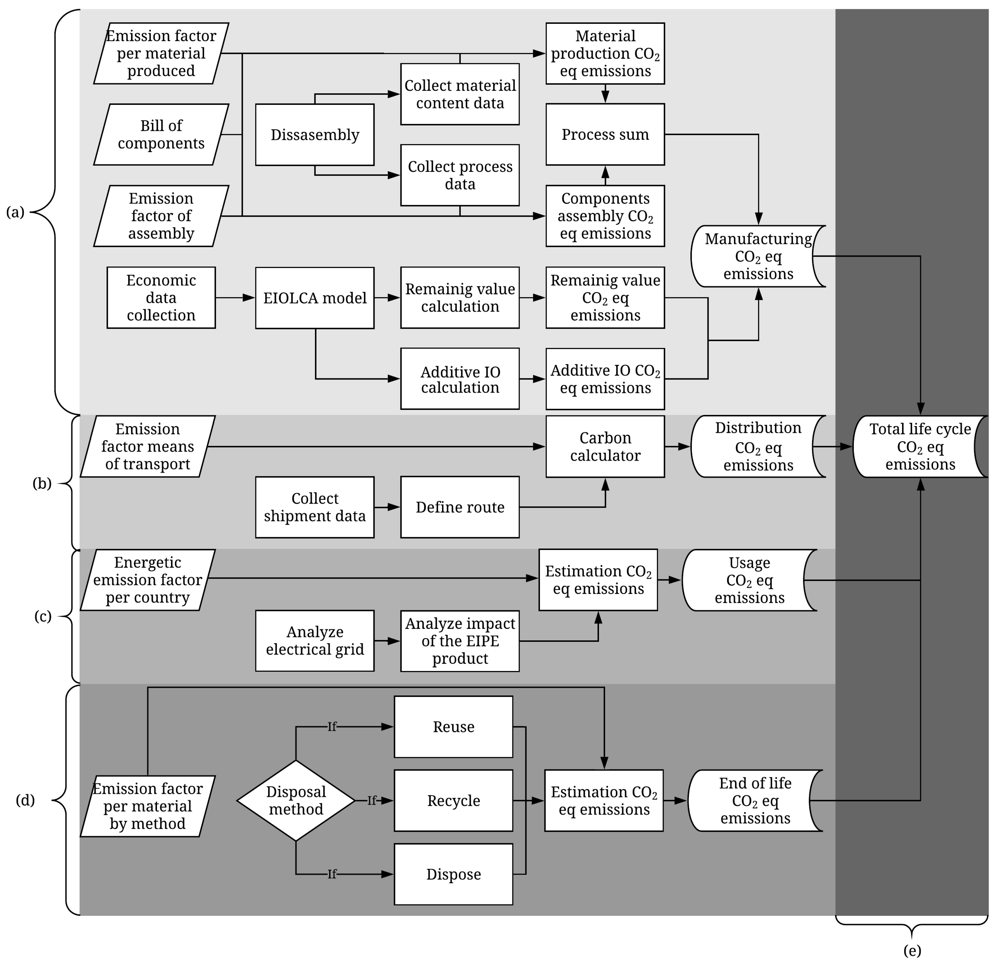Figure 1 shows a scheme of the methodology applied to perform the CF estimation.

Figure 1 shows the entire methodology to estimate CF using an LCA approach per stage. Estimation in (a) is based on the hybrid LCA method from cradle to gate. Estimations in (b), (c), and (d) are based on standards ISO 14067 [20] and PAS 2050 [19], allowing the estimation of CF in the distribution, usage, and end-of-life stages. Finally, in the final step (e), the CF estimations from previous stages are added up to generate an approximate estimate of CF in the life cycle of an EIPE product.

Stage (a) takes into account processes related to raw extraction material and to manufacturing of an LCA. In this stage, an economic balance model is used to estimate CF similar to the estimation of CF for electronic products proposed by References [3,23]. In stage (a), it is required to divide the analysis into two sections. The first section has inputs as the bill of components, the emission factor related with extraction per material used in the product, and the emission factor related with the assembly of components. The next step considers the disassembly of the EIPE product which comprises material content data and information about the processes involved. Then, with the weight of the materials, CO₂eq emissions are estimated using the corresponding $EF$.

In stage (a), the second section takes into account CO₂eq emissions that are not considered in the bill of components using an economic balance. This method uses economic data which is processed in the Economic Input-Output Life Cycle Assessment (EIOLCA) model [24]. This model estimates two economic correction factors: remaining value and additive input–output (IO). After, these correction values are extrapolated to CO₂eq emissions. Finally, results from the economic data and the material data are added up in order to get manufacturing CO₂eq emissions [3,23].

Stage (b) estimates CO₂eq emissions related to the distribution of a product. It starts collecting shipment data related to the product as weight, volume, and packaging. In the next step, a route should be defined from the factory to the customer, specifying the type of transport. All this information feeds a carbon calculator [25], which gives the emissions associated with the distribution stage.

Stage (c) estimates the CO₂eq emissions related to usage of the product. EIPE products have a direct impact on the electrical grid. Thus, the analysis requires definition of the electrical grid where the device will be used. After this definition, the impact of the product on the electrical grid is analyzed in terms of the energy consumed during its useful life. It is important to highlight that a calculation of saved energy ($SE$) must be included for a more realistic CF estimation. Many EIPE products are installed in power networks to improve processes or to solve some limitations. In general terms, they are directly or indirectly used to increase the electric power system efficiency so that EIPE products facilitate the reduction of the energy consumption; thus CF emissions are significantly reduced in most cases.

Stage (d) estimates the CO₂eq emissions related to end-of-life of the product. This stage is different from the previous ones because it takes into account three methods of disposal: reuse, recycle, and disposal. Each one has its own implications with a direct relationship with the location of the product [26]. Estimation of CO₂eq emissions uses an $EF$ factor per material per method of disposal in a specific place.

Finally, the results of manufacturing, distribution, usage, and end-of-life stages are added up to obtain total life cycle CO₂eq emissions.

2.1. Hybrid LCA to Estimate CF in Cradle-to-Gate Scenario

The integrated hybrid analysis, described in stage (a) of Figure 1, is the most appropriated method to estimate CF of an EIPE product. This method uses the computational mathematical structure of LCA, along with input–output analysis and an economic balance. It collects data on materials and components directly from the dismantling of the product rather than relying on general databases or published material data. In addition, it collects data on energy consumption at the process level through industrial reports and literature review for stages of extraction and production of bulk materials, production and assembly of the components of the product, and its final manufacture. To assure the minimum cut-off error, this approach adds an Economic Input–Output (EIO) correction to check inputs in the supply chain that are not involved in the process-sum inventory. The EIO correction is composed of two factors: additive and remaining value (RV) [27]. The additive factor accounts for product components with specific economic data on requirements per product, omitting involved processes. The RV estimates the contribution from all the remaining, unaccounted sectors based on the available economic value of the product [23]. Equation (1) depicts a simplification of the model:

$$E=E^{Process}+E^{Additive}+E^{RV}$$

(1)

where $E^{Process}$ represents energy used in processes considered in the analysis (for example, semiconductor fabrication and board circuits assembly). $E^{Additive}$ represents the involved portion of other industries that are not directly considered in the $E^{Process}$ because the process data are restricted (for example, using the price of the chemicals used in the assembly due to the lack of knowledge of the process of its manufacture). Also, economic input–output models are formulated in terms of the producer or purchase prices. The production cost is the price of the product when it leaves the factory, while the customer price considers the cost of manufacturing, transportation, distribution, and sales margins [28].

Finally, $E^{RV}$ estimates the contributions of the processes using an EIO model to generate the economic contribution of the sectors involved. This approach considers the RV in the manufacturing process that is not covered in the additive or process analysis [29].

2.2. Distribution Stage

In the shipment of merchandise, CF refers to direct consumption of energy and/or fuel. Companies move their merchandises by air, land, and sea transport. Because of this diversity, a simplified equation based on ISO 14067 [20], PAS 2050 [19], and the GHG Protocol [30] is implemented. Stage (b) of Figure 1 describes in detail how to estimate the CF related to distribution. This estimation considers measurements of different types of transport to ship the merchandise until its final destination.

$$TE=\sum M\times D\times EF$$

(2)

where TE is the total GHG emissions in kg CO₂eq related to the shipment and M refers to the mass (kg) of the merchandise when it is transported by air or land. When considering sea transportation, M refers to the occupation volume (m³). D is the distance traveled during transport, and $EF$ is a specific emission factor (g CO₂eq/km) that considers relevant load factors to allocate CO₂eq emissions.

2.3. Usage Stage

The estimation of CF in the usage stage of an EIPE device starts as an estimate for an electronic device based on PAS 2050 [19] and ISO 14067 [20]. The equation proposed in these standards estimates the annual average of energy emission factors for specific countries, considering the average energy consumption of the device in the country. Equation (3) shows the expression for the estimation:

$$TE=T\times C\times EF$$

(3)

where $TE$ is the total GHG emissions during their useful life (g CO₂eq); T is the average time the device is working (h); C is the average electric power consumption (kWh), which depends strictly on the designer; and $EF$ is the specific emission factor that depends on how electricity is generated in the country where the device is located (g CO₂eq/kWh).

However, to determine the impact of using the EIPE device on the electric grid, it is necessary to account for generated emissions with and without the device in the electric network. This estimation is performed by means of Equation (3) as described in stage (c) of Figure 1. Thus, $\Delta TE$ is proposed, which allows for the consideration of the difference between the CF of the electrical network with or without EIPE throughout its useful life. The result can be positive, negative, or zero. If it is negative, the results represent the saved emissions during the useful life of the device. If it is positive, the results show the total emissions generated during the useful life of the device. If it is zero, the electricity grid does not suffer changes in its emissions with or without a device.

2.4. End-of-Life Stage

When a product reaches the end-of-life, it can be recycled, reused, or disposed of. Methods that consider emissions in this stage are based on PAS 2050 [19] and depend on the final treatment given to the EIPE product or any other electrical product. When an electrical product reaches end of life, it cannot be used to produce energy through combustion because of its properties. Section (d) of Figure 1 shows the options to dispose of EIPE products. If the EIPE product is disposed of like waste in a landfill, it will not generate considerable GHG emissions because it is not composed of organic matter. The remaining disposal methods, reuse and recycling, generate considerable emissions.

2.4.1. Treatment of Emissions Associated with Reuse

Reuse refers to giving new use to some part of the product instead of discarding it. PAS 2050 [19] considers the next expression to simplify the calculation of GHG emissions through Equation (4):

$$\mathrm{GHG}\mathrm{emissions}=\frac{a+f}{b}+c+d+e$$

(4)

where a is the total life cycle GHG emissions of the product, excluding use-phase emissions; b is the anticipated number of reuse instances for a given product; c refers to emissions arising from an instance of the refurbishment of the product to make it suitable for reuse; d refers to emissions arising from the use stage; e is emissions arising from transport returning the product for reuse; and f is emissions arising from disposal [19].

2.4.2. Treatment of Emissions Associated with Recycling

Recycling transforms matter using energy demand to execute it. PAS 2050 [19] presents different options to assess emissions related with this process, depending on the transformation that suffers the product. One method considers that the recycled material does not maintain the same inherent properties as the virgin material input; for this case, emissions are estimated using Equation (5). The other method considers that recycled material maintains the same inherent properties as the virgin material input; for this case, emissions are estimated using Equation (6). Selection of the method depends on the knowledge of the material and its capacity to be recycled.

$$E=(1-R_1)E_V+R_1{E}_R+(1-R_2)E_D$$

(5)

$$E=(1-R_2)E_V+R_2{E}_R+(1-R_2)E_D$$

(6)

where $R_1$ is the proportion of recycled material input; $R_2$ is the proportion of material in the product that is recycled at end-of-life; $E_R$ are emissions and removals arising from recycled material input per unit of material; $E_V$ are emissions and removals arising from virgin material input per unit of material; and $E_D$ are emissions and removals arising from disposal of waste material per unit of material.

As mentioned before, in these stages, the location of the product is important to estimate the CF. When considering the recycling process, data availability of $EF$ per material in each location limits the estimation of GHG emissions. Moreover, comparison of GHG emissions is complex because of the differences encountered in the collection and recycling methods of materials according to the technological level applied [31] for different locations. However, different methods to obtain recycling $EF$ per material are based on ISO 14067 and PAS 2050 standards, which is why emission factors are directly applied in the proposed methodology.

2.5. Total Life Cycle Carbon Equivalent Emission

LCA stages are consecutive and interlinked and represent a portion of the total CF of the product. Therefore, to obtain the total CF for the EIPE product using a life cycle assessment, CF estimations for stages (a), (b), (c), and (d) are added up to get the total CF (stage (e)).

3. Results

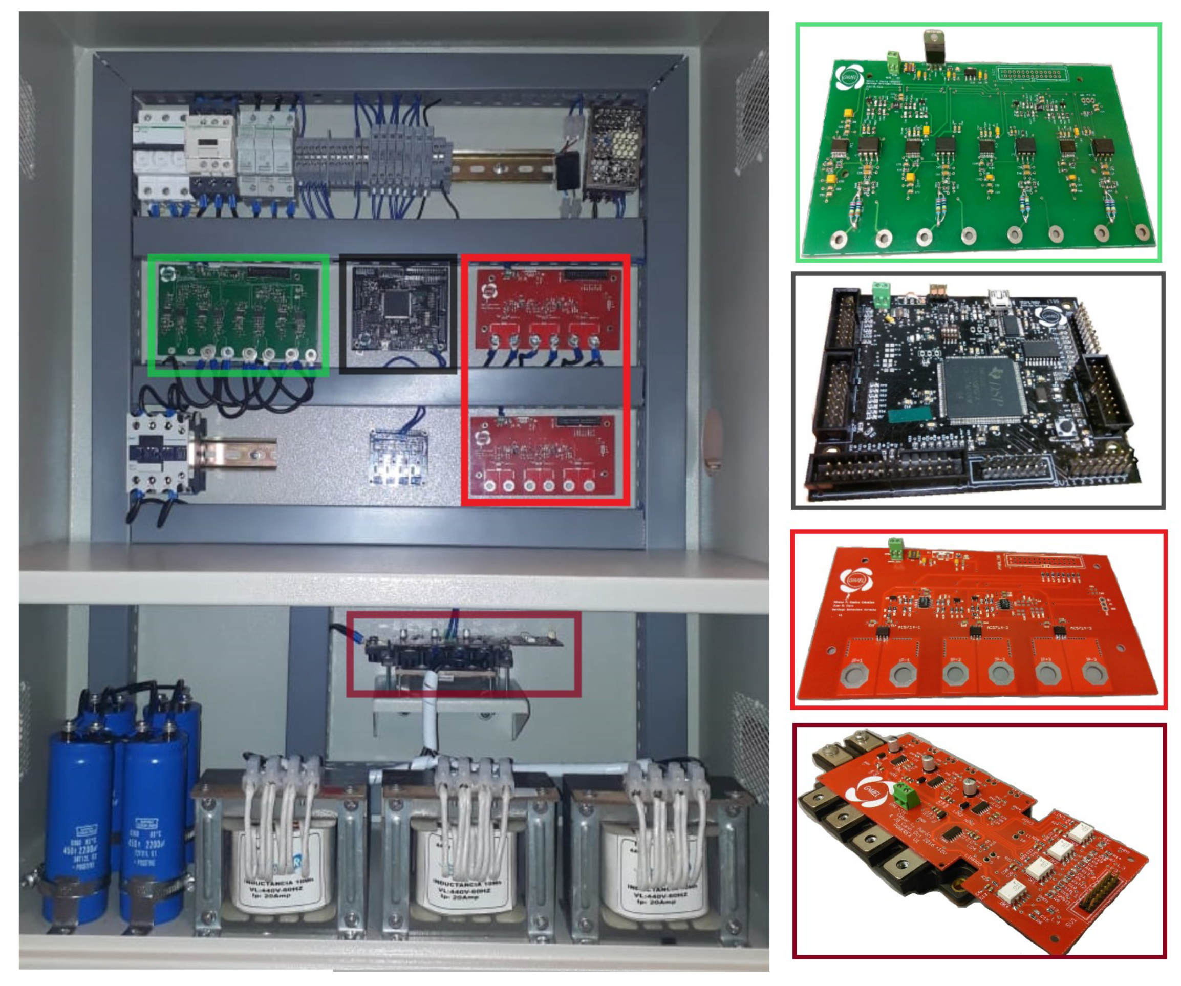
In this section, the multi-pronged approach discussed above to estimate CF in a cradle-to-grave scenario is applied to a Distribution-Static Var Compensator (D-STATCOM) prototype of 30 kvar. The D-STATCOM analyzed is shown in Figure 2.

The D-STATCOM has more than 100 components. Most of the components were analyzed through data sheets provided by the producer of the components. Parts without available data were weighted using a microbalance. Also, to perform the estimation of stage (a), components of material were identified and version 2.2 of the database provided by the association EcoInvent in Zurich (Switzerland) [32] was used to obtain information on CO₂eq emitted during materials extraction. GHG emissions involved in the manufacturing stage were estimated during the development of the D-STATCOM. However, CF estimation does not correspond strictly to an integration of the supply chain of the product due to CF estimations depending on data available or a correlation with similar products.

Emissions related to manufacturing, assembly of the D-STATCOM, and its functional tests are measured as direct emissions with control of the operator in the laboratory.

3.1. CF through Economic-Balance Hybrid LCA

In this section, we use the hybrid LCA method by Deng et al. [23] and Vasan et al. [3], described in Equation (1), which considers two correction factors. $E^{Additive}$ takes into account emissions resulting from relevant industries. These emissions are obtained using the EIOLCA model [24] in which specific economic data on requirements per product are available. $E^{RV}$ estimates the emission contributions from processes for which neither materials nor economic data are publicly available.

3.1.1. Process Data Analysis

The D-STATCOM contains four circuit boards, four electrolytic capacitors, one power transistors module, four inductors, one box support, and more than 100 micro-components and support pieces as shown in Figure 2. The production-related emissions of materials were obtained from measurements of weight, material composition, and data available from the EcoInvent databases [32].

Table 1. Embodied CO₂eq in materials.

Material	Amount per Converter (kg)	CO2eq Intensity (kg CO2eq/kg)	CO2eq per Converter (ton)
Aluminum	32.78	8.24	0.270114
Arsenic	0.04	4	0.000145
Brass	0.03	4.39	0.000153
Cadmium	0.00	5.8	0.000002
Carbon	0.10	6.5	0.000648
Ceramic	0.15	5.5	0.000841
Copper	8.63	3.5	0.032747
Epoxy	0.70	9	0.006321
Fiber glass	0.0002	8.1	0.000002
Glass	0.002	0.85	0.000001
Gold	0.02	3000	0.048786
Iron	0.19	1.91	0.000368
Lead	0.00	20	0.000026
Manganese	0.10	2.6	0.000289
Nickel	0.19	12.4	0.002323
Nylon	0.06	6.5	0.000420
Phosphor	0.02	3.39	0.000081
PVC	0.08	2.2	0.000343
PBT	0.08	7.9	0.000647
Silicon	0.29	10	0.002880
Silver	0.20	754	0.150227
Steel	13.85	5.9	0.081720
Tantalum	1.21	260	0.313812
Tin	0.28	13.7	0.003888
Zinc	0.07	9	0.000596
Total	59.07	-	0.917350

lists the main materials found in the D-STATCOM with the highest associated emissions, considering material composition and the energy consumption during the component production (see stage (a) in Figure 1). CO₂eq from the D-STATCOM bulk materials is estimated to be around 0.91735 ton CO₂eq.

Table 2. Embodied CO₂eq in manufacturing and assembly processes.

Process	Time (h)	Avg. Energy Consumption (kWh)	CO2eq Intensity (g CO2eq/kWh)	CO2eq per Converter (ton)
Assembly D-STATCOM	1.5	0.22	182	0.000060
Functional tests	1	15	182	0.002730
Total	2.5	-	-	0.002790

summarizes the associated assembly process emission data, estimated as energy consumption per hour in the factory (the laboratory where the prototype was developed) located in Medellín (Colombia). This estimation corresponds to the “Components assembly CO₂eq emissions” shown in stage (a) of Figure 2. Other processes involved in the production of pieces are considered in Section 3.1.2. The total life cycle CO₂eq emissions for this section is around 0.00279 ton CO₂eq. However, the chemicals used in bulk materials production, D-STATCOM manufacturing, and functional tests were not taken into consideration in the process-sum analysis.

Finally, total CO₂eq emissions associated with the process section are 0.92014 ton CO₂eq and correspond to the $E^{Process}$ contribution in Equation (1).

3.1.2. Economic Input–Output Correction

The economic value of the electronic chemicals used to manufacture the D-STATCOM is obtained based on the expenses involved in the processes mentioned in Table 2, corresponding to $E^{Additive}$. The estimation considers the amount of electronic chemicals used per device. The value obtained is approximately $5.5 in 2018 per device. This value has to be adjusted to the 2002 US dollar monetary unit in order to use the US 2002 Benchmark model purchaser price from the EIOLCA model. This value corresponds to $4 in 2002.

$E^{RV}$ estimates the contribution of processes that are not included in either process-sum analysis or additive IO. The producer price in 2018 of the D-STATCOM was $1775 in 2018, which was adjusted to the dollar value in 2002, that is $1268.

Table 3. Remaining Value (RV) input–output (IO) correction calculation and embodied CO₂eq per D-STATCOM.

	Value per Converter ($)	Fraction Accounted (%)	Value Accounted for Analysis ($)
Process-sum
1. Breakers	$155	38	$59
2. Electrolytic capacitor	$262	38	$100
3. Circuits boards	$17	40	$7
4. Transistor	$76	38	$29
5. Bulk materials	$396	45	$178
6. Manufacturing	$357	41	$146
7. Support box	$114	88	$101
Additive IO
8. Electronic chemicals	$4		$4
Total value accounted in process-sum and addition IO			$620
Producer price in 2002 USD			$1268
Producer price in 2018 USD			$1775
Remaining Value (RV)			$652
Total RV per D-STATCOM (ton CO2eq)			0.321

shows the values estimated with the EIOLCA model [24]. The results show that $620 account for the process-sum analysis and the additive estimation. Then, RV is approximately $652 in 2002. In this estimation, the fraction accounted for the sum of processes was determined by selecting the related economic sectors of the 2002 model Benchmark purchaser price from the EIOLCA. The model has 247 economic sectors; then, the related sectors of each component manufacture are selected. However, the economic sectors involved in the previous steps must be omitted to estimate the RV. The top 39 selected sectors represent 99.9% of RV shares, but around 7–12 sectors per each component were removed in order to avoid double counting.

Then, it was only considered 82% of $E^{Additive}$ and $E^{RV}$ with a value of $652 in 2002. According to The Bank Group analysis, CO₂ emissions per USD depend on the GDP [33]; this quantity corresponds to 0.321 ton CO₂eq.

Finally, the previous results are added up following Equation (1) to obtain CO₂eq emissions associated with stage (a) in Figure 1. The total CO₂eq emissions in the manufacturing stage are 1.24107 ton CO₂eq.

3.2. CF Estimation Using Standards After the Product Leaves the Factory

In this section, the final location of the D-STATCOM has to be taken into account. However, there is no control in the stages of distribution, usage, and final disposal. To estimate CF, it is considered that the device will be distributed, used, and disposed of in two different countries: Stockholm (Sweden) and Macau (China). These countries are selected because Sweden is the country with the cleanest energy matrix and China has an energy matrix that generates significant GHG emissions [34,35].

3.2.1. Exporting a New Reactive Power Compensation D-STATCOM

This section shows how to obtain CO₂eq emissions related to stage (b) in Figure 1, which considers the distribution of the device. The D-STATCOM will be sent from Medellín (Colombia) to Buenaventura (Colombia) by road and continue their trips by sea to the final destination (either China or Sweden). GHG emissions were estimated through Equation (2) using a carbon calculator [25]. The calculator allowed using data to simulate in real time the shipping route and corresponding CF estimation. This tool is used because it is based on the guidelines outlined in the GHG Protocol [30] and follows the requirements by European Emissions Trading System (EU-ETS) [36], EN 16258 [37] (based on PAS 2050 [19]), and ISO 14067 [20]. In Equation (2), weight and volume of the D-STATCOM are 68.4 kg and 0.4 m³, respectively. These values were considered for different types of transport involved in the route to reach the final destination. Emissions factors were also obtained from the carbon calculator [25]. The CFs associated with the shipment of the device to Sweden and China are 0.0176 and 0.0226 ton CO₂eq, respectively. Values used to estimate CF for the distribution stage are described in

Table 4. EIPE product distribution stage.

Destination	Distance Road (km)	EF by Road (kg CO2eq/kgkm)	Distance Sea (km)	EF by Sea (kg CO2eq/kgm3)	TE CO2eq (ton)
Stockholm (Sweden)	471.61	0.0000837	11671.21	0.0031959	0.017620
Macau (China)	471.61	0.0000837	18327.30	0.00271453	0.022600

.

3.2.2. D-STATCOM in a New Location

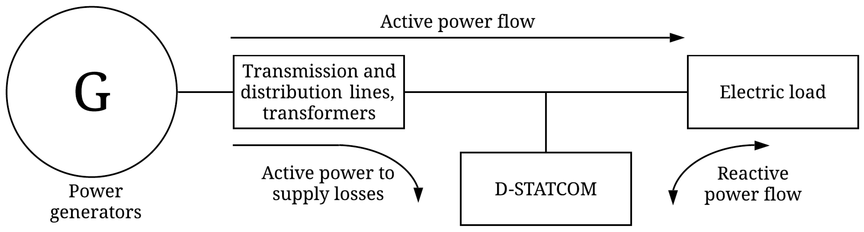
D-STATCOM was chosen as the case to be analyzed due to the fact that it is an EIPE device that significantly contributes to the improvement of the efficiency. Figure 3 shows a power system that is composed of (1) power generators in charge of energy generation; (2) transmission lines, distribution lines, and transformers in charge of energy transportation; (3) an electric load that demands the electricity, transforming it in other forms of energy; and, of course, (4) a D-STATCOM in charge of reactive power compensation. When the D-STATCOM is not connected, power generators must deliver active and reactive power flows in order to satisfy the requirements of the electric load. Active and reactive power flows cause losses in transmission lines, distribution lines, and transformers.

Active power is a useful power, while reactive power is an inefficient power and must be compensated to obtain high standards of power quality and efficiency. For this reason, D-STATCOMs are connected in parallel near to the electric load for compensating the reactive power flow and avoiding its circulation through the power system; thus, power generators can supply an equivalent quantity of active power (useful power) to other loads. After the compensation, reactive power bidirectionally flows between the D-STATCOM and the load; however, a small quantity of active power is required to satisfy D-STATCOM internal losses.

CF of the usage stage, as depicted in stage (d) in Figure 1, is estimated using Equation (3). The $\Delta TE$, which allows assessing the impact of the incorporation of the device, is determined considering the difference of emissions between a power grid with and without the application of an EIPE product. For this, it was estimated that the D-STATCOM has a useful life of 15 years and its efficiency is 95%, while efficiency of transmission systems is typically 80%. It is estimated that the energy expenditure on the power system without the device is 788.4 MWh and with the device is 236.5 MWh throughout its useful life. The $EF$ used for each of the two countries is taken from the Organization for Economic Cooperation and Development [38]. $\Delta TE$ obtained for Sweden is −7.2 ton CO₂eq and for China is −392.4 ton CO₂eq. The negative sign means that the incorporation of the device results in saved emissions in both countries. Results are shown in

Table 5. CO₂eq emissions for the usage stage per location.

Location	EF 2013 (g CO2eq/kWh)	TE Case without Device (ton CO2eq)	TE Case with Device ton CO2eq)	ΔTE (ton CO2eq)
Stockholm (Sweden)	13	10.2	3.0	−7.2
Macau (China)	711	560.6	168.2	−392.4

.

In Table 5, $\Delta TE$ values for Sweden and China vary considerably although the electrical network where they are applied is the same. Therefore, the energy $EF$ per country is what causes the difference in the results. Even though the D-statcom saves the same amount of kW in both countries, the device application in China saves more emissions than in Sweden because the Chinese $EF$ per kW is one of the largest in the world. Consequently, the environmental benefit of our D-statcom is directly proportional to the energetic emission factor.

3.2.3. End-of-Life of the Product

The electronic industry generates scraps which are not degradable. Moreover, reuse of some parts or components is limited because producers prefer to use a new component for its products even if it is possible to utilize a used part. Electronic products are difficult to recycle due to its size. Also, the recycling processes of the unions of electronic components are expensive. Then, it is cheaper to make new electronic components than to try to recycle them. However, metal components and cabling in the electronic devices are recycled because they are considered metallic waste [39].

For the reasons mentioned above, it is considered that only metal parts and cabling of the device are totally recycled. The prototype has 3 metal parts that represent about 80% of the total weight: the support box, craft coils, and cabling. The other 20% are components considered electronic waste with low CO₂ emissions.

Equation (6) was used to estimate emissions related to the recycling process of the D-STATCOM, which is considered in stage (d) in Figure 1. It is supposed that the device will be separated by macro-components and that these will be divided by metals if possible. In addition, it is considered that the parts that are totally metallic are recycled at the end of their useful life. Based on Equation (6), in Sweden, $E_R$ associated to aluminum and steel recycling was estimated by Hillman et al. [40] and $E_R$ associated with copper recycling was approximated by Agency [41]. In China, $E_R$ associated to aluminum and steel recycling was estimated by Reference [26] and $E_R$ associated with copper recycling was estimated by Reference [42]. The results are shown in

Table 6. Embodied CO₂eq in recycling materials.

Material	Weight (kg)	CO2eq Intensity (kg CO2eq/kg)		CO2eq per Converter (ton)
		Sweden	China	Sweden	China
Aluminium	31.8	0.4	1.26	0.01272	0.040068
Copper	8.9	1.5	2.94	0.01338	0.026231
Steel	12.7	0.3	1.02	0.00381	0.012942
Total	-	-	-	0.02991	0.079240

.

The estimates of the end of life stage for this scenario were simplified because there was not enough data available on the level of technology and the capacity of the factories for each metal in the countries where the product is located. CO₂eq emissions for aluminum, copper, and steel were respectively 0.01272, 0.01338, and 0.00381 ton CO₂eq for Sweden and 0.04007, 0.02623, and 0.01294 for China. Then, total emissions associated with stage (d) in Figure 2 are obtained, adding up emissions generated by the recycling of each metal. The total emissions for this stage are 0.02991 and 0.07924 ton CO₂eq for Sweden and China, respectively.

3.3. Total Life Cycle CF of an EIPE Product

As stated in Section 2.5, the sum of all stages described in Figure 1 results in the CF of the entire life cycle of the product; this corresponds to stage (e). Hence, emissions related to the EIPE manufacturing using an integrated hybrid LCA approach are 1.241 ton CO₂eq (see Table 1, Table 2 and Table 3). The next stages were estimated based on PAS 2050 and ISO 14607 standards considering Sweden and China as reference countries. The distribution emissions were 0.020 ton CO₂eq in Sweden and 0.024 ton CO₂eq in China. Usage stage emissions consider the difference in emissions generated in an electric system with and without the EIPE device. Saved emissions are 7.2 ton CO₂eq in Sweden and 392.4 ton CO₂eq in China. End-of-life emissions through metal recycling are 0.029 and 0.079 ton CO₂eq in Sweden and China, respectively. Finally, according to

Table 7. Embodied CO₂eq in recycling materials.

Country	Manufacturing (ton CO2eq)	Distribution (ton CO2eq)	Usage (ton CO2eq)	End-of-Life (ton CO2eq)	Total LCA Emissions (ton CO2eq)
Sweden	1.24107	0.017620	−7.2	0.02991	−5.88
China	1.24107	0.022600	−392.4	0.07924	−391.04

, the total life cycle CO₂ emissions are −5.88 ton CO₂eq in Sweden and −391.04 ton CO₂eq in China. The results show that the incorporation of an EIPE device in a power system allows saving CO₂ emissions in both countries.

In general terms, emissions are mainly produced in the manufacturing stage; in this stage, most of the emission is generated in the process of raw extraction material. Producers could improve their designs by trying to use alternative materials to aluminum and silver where emissions are concentrated. Additionally, economic input–output correction is necessary due to RV corresponding to nearly 25% of emissions produced in the manufacturing stage. Compared with the manufacturing stage, the distribution and end-of-life stages do not significantly produce CO₂ emissions; however, the highest emissions in an LCA were presented at the usage stage, but when considering the electrical implications of the device on the network, it results in saved emissions. This implies that CF is decreased and, at the same time, contributes to the energy efficiency of the system even though the energy comes from the same generator. The results show that the usage stage has a positive environmental impact which is consistent with a negative CF and contributes to getting a CF overcompensation in the total estimation. Because emissions saved due to the reduction of energy consumption are greater than the sum of the emissions of all the other stages, it is recommended to install D-STATCOMs or EIPE products as long as they contribute to the improvement of energy efficiency. In conclusion, EIPE products generate environmental benefits superior to the impacts generated throughout the life cycle of the product. Therefore, it is considered that EIPE products can help to comply with energy efficiency policies stipulated in international agreements like the Kyoto protocol or COP 21. In particular, EIPE products help to reduce energy, which is in line with energy efficiency resource standard policies or strategic energy management plans. In this regard, governments can implement in their strategic plans the incorporation of reactive power compensation devices at transmission line strategic points to improve their energy efficiency and to thus decrease their CF.

4. Conclusions

The proposed methodology for estimating CF of EIPE products considers a multi-pronged assessment that was achieved using three scopes: (1) direct emissions (owned operations), (2) indirect emissions (energy consumption), and (3) indirect emissions (downstream transportation and distribution). Also, the methodology was designed to be applied to a cradle-to-grave scenario which is composed of an integrated hybrid approach and a standard based approach (ISO 14067 and PAS 2050). The methodology was explained in detail and is presented as a complete methodology to estimate CF during the life cycle of the product. Schematic diagrams to link all stages of the methodology were included to provide a better understanding. EIPE products are designed to contribute to efficiency improvement, so an energy calculation is presented in the usage stage in order to refine CF estimation.

The proposed methodology allows for the estimatation of CF for the distribution stage, considering different scenarios for the transportation. This feature is useful when considering the application of these estimations to propose mitigation actions that seek to reduce GHG emissions. Another highlight of the methodology applied to EIPE products is the estimation of the usage stage, which is not considered in other approaches. This estimation allows for the consideration of environmental implications of the incorporation of an EIPE device in an electrical grid.

The methodology was applied to a 30 kvar D-STATCOM manufactured in Colombia. A comparative analysis was made in two countries with very different energy matrices, Sweden and China. The difference between the possible emissions in the electrical grid with and without the device was estimated. Taking into account the useful life, it was found that CF for both countries is totally compensated, and furthermore, a negative CF (overcompensation) occurs, which is considered as a beneficial environmental impact. It can be concluded that the emissions saved due to the reduction of energy consumption in the usage stage are greater than the sum of the emissions of all the other stages of its life cycle, so a calculation of the energy saved during the operation of EIPE products is absolutely essential for a more realistic CF estimation.

The results exhibit a great difference between the Swedish and Chinese environmental impacts. The ton CO₂eq saved for Sweden was 5.88 while for China was 391.04. The reason for this is that the energy matrix for Sweden is mainly composed of renewable or clean sources while China has a diversified energy matrix (based on coal, oil, solar PV, and wind, among others). Therefore, it is recommended to prioritize the installation of EIPE products in countries where the energy matrix includes fossil fuels to significantly reduce/compensate CF. This feature of an EIPE device would facilitate nations to reduce their CF related to the energy sector, as it is stated in the COP 21 international agreement.

Finally, there is a limitation in the end-of-life stage since the values of the $EF$ are not estimated under the same parameters because, in each country, the collection methods and the technological level in the transformation of materials vary according to waste recycling plants. However, emission factors which are estimated based on ISO 14067 and/or PAS 2050 were considered comparable for the proposed methodology. To solve this limitation, it is recommended that the governments be obligated to report the GHG emissions per material emitted by waste recycling plants as is mentioned in the COP 21 agreements.