Evaluation of Photovoltaic Power Generation by Using Deep Learning in Solar Panels Installed in Buildings


Department of Marine Environmental Informatics & Center of Excellence for Ocean Engineering, National Taiwan Ocean University, No.2, Beining Rd., Jhongjheng District, Keelung City 20224, Taiwan
Energies 2019, 12(18), 3564; https://0-doi-org.brum.beds.ac.uk/10.3390/en12183564
Submission received: 14 August 2019
/
Revised: 14 September 2019
/
Accepted: 15 September 2019
/
Published: 17 September 2019
(This article belongs to the Special Issue Renewable Energy Resource Assessment and Forecasting)
Abstract
:Southern Taiwan has excellent solar energy resources that remain largely unused. This study incorporated a measure that aids in providing simple and effective power generation efficiency assessments of solar panel brands in the planning stage of installing these panels on roofs. The proposed methodology can be applied to evaluate photovoltaic (PV) power generation panels installed on building rooftops in Southern Taiwan. In the first phase, this study selected panels of the BP3 series, including BP350, BP365, BP380, and BP3125, to assess their PV output efficiency. BP Solar is a manufacturer and installer of photovoltaic solar cells. This study first derived ideal PV power generation and then determined the suitable tilt angle for the PV panels leading to direct sunlight that could be acquired to increase power output by panels installed on building rooftops. The potential annual power outputs for these solar panels were calculated. Climate data of 2016 were used to estimate the annual solar power output of the BP3 series per unit area. The results indicated that BP380 was the most efficient model for power generation (183.5 KWh/m2-y), followed by BP3125 (182.2 KWh/m2-y); by contrast, BP350 was the least efficient (164.2 KWh/m2-y). In the second phase, to simulate meteorological uncertainty during hourly PV power generation, a surface solar radiation prediction model was developed. This study used a deep learning–based deep neural network (DNN) for predicting hourly irradiation. The simulation results of the DNN were compared with those of a backpropagation neural network (BPN) and a linear regression (LR) model. In the final phase, the panel of module BP3125 was used as an example and demonstrated the hourly PV power output prediction at different lead times on a solar panel. The results demonstrated that the proposed method is useful for evaluating the power generation efficiency of the solar panels.
1. Introduction
Solar photovoltaic (PV) energy systems generate electricity without causing pollution. Moreover, grid-connected PV cells can easily be installed on residential building roofs and commercial building walls [1]. In Taiwan, the solar energy industry has become popular; various PV power generation systems can be installed in buildings for improving energy-use efficiency. Because Taiwan is located in a subtropical region, it receives abundant sunlight and is suitable for developing solar energy. Solar cells, also known as PV cells, directly convert solar energy to electricity. Solar energy has become an alternative energy used in Taiwan because it does not cause environmental pollution or noise.
Solar cells convert sunlight to electricity through the PV effect, in which an appropriate energy-level design is employed to effectively absorb sunlight and convert it to electric voltage and currents; this conversion process is known as photovoltaics. Numerous semiconductor materials are available for solar power generation. Silicon, a prominent raw material for solar cells, is commercially divided into monocrystalline, polycrystalline, and noncrystalline silicon. Monocrystalline and polycrystalline silicon materials exhibit the same power generation mechanism despite differences in their crystal structures. The cell temperature mainly depends on the irradiance intensity and ambient temperature [2]. Semiconductors are temperature-sensitive; after the cell temperature exceeds 25 °C, each increase of 1 °C reduces the overall efficiency of monocrystalline, polycrystalline, and noncrystalline silicon cells by 0.71%, 0.5–0.66%, and 0.2–0.3%, respectively [3]. Currently, polycrystalline silicon solar cells are dominating the solar cell market, representing 90% of the market sales, with a 20–30% market growth. In 2017, silicon-based solar cells could generate PV power of up to 55 GW; this value is estimated to reach 100 GW by 2020 [4].
Solar power generation is a form of environmentally friendly power generation method, in which no greenhouse gases, such as carbon dioxide, are generated. However, solar radiation is absorbed, reflected, or refracted by clouds of varying thicknesses after entering the atmosphere, which cause an inconsistency in solar radiant energy sources. When the density of energy collected by a set of solar panels is low, several additional solar panels must be installed, which increases their investment costs. Approximately 45% of the cost of a silicon cell solar module is determined by the cost of the silicon wafer. Thus, efforts are being made to use less silicon in the manufacture of solar cells [5]. Therefore, appropriate solar panels must be selected while developing a rooftop PV system in Taiwan. Previous studies have evaluated PV power generation panels of various geometries for different buildings [6,7,8]. For example, Jeong et al. [9] used amorphous silicon PV panels to develop prototype models of blinds with smart photovoltaic systems. Mahmud et al. [10] presented an environmental lifecycle assessment of a solar PV system by using single crystalline Si solar cells and a solar thermal system that used evacuated glass tube collectors. Kouhestani et al. [11] used a multi-criteria approach based on geographic information systems and light detection and ranging (LiDAR) to estimate rooftop PV electricity potential of buildings in an urban environment. Additionally, for evaluating the solar panel suppliers, several studies have used multi-criteria decision making (MCDM) approaches in various fields of science and engineering [12,13]. For example, Wang and Tsai [14] presented a fuzzy MCDM approach using a fuzzy analytical hierarchy process model and data envelopment analysis for selecting solar panel suppliers for a photovoltaic system design in Taiwan.
Seasons, daytime length, the Earth’s revolution and rotation, and climate changes affect the reception of solar energy [15]. The Earth’s revolution and rotation are regular and can be accurately calculated using mathematical models, but the atmospheric conditions (e.g., clouds, temperature, and wind velocity) of Taiwan, which has an island climate, change rapidly and are difficult to forecast. Therefore, solar radiation must be accurately predicted in advance to accurately evaluate the total power generated through rooftop PV systems and their overall efficiency. A surface solar radiation prediction model should be established for this purpose.
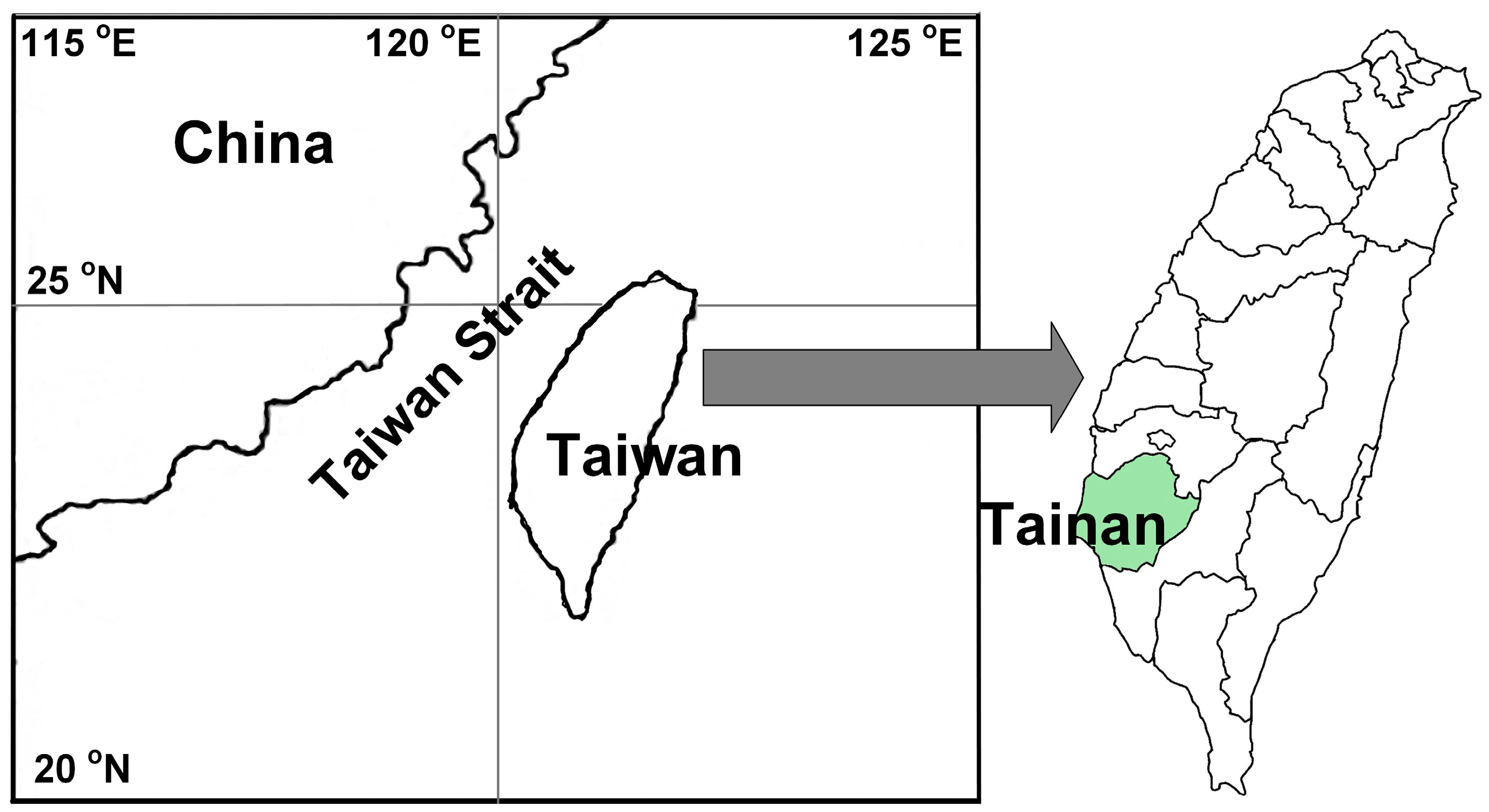
The aforementioned problems indicate that efficient and prompt evaluation of the power generation efficiency of specific solar panel brands is essential in planning the installation of rooftop PV systems in Taiwan. Therefore, this study has three objectives: (1) evaluation of the potential annual power outputs of selected solar panels, (2) prediction of future hour-based solar radiation levels, and (3) assessment of the annual power for a specific solar panel when the forecasting horizon increases. The study site was Tainan (Figure 1), where the average annual solar irradiance was 1.65 MWh/m2-y according to the statistical data from 2010 to 2016. Tainan, which has a stable climate and frequent sunshine, is suitable for solar power generation in all seasons.
Most rooftop PV systems in Taiwan are fixed. Therefore, the solar radiation received by solar panels at different inclination angles must be estimated. The amount of solar radiation incident on a solar thermal collector or a PV panel is strongly affected by its installation angle and orientation [16]. Over the past decade, various models have been proposed for predicting solar radiation on inclined surfaces [17,18,19,20]. Maleki et al. [21] reviewed several models for estimating solar radiation components on horizontal and inclined surfaces. As indicated by [16], all these models require hourly global irradiations and hourly horizontal diffuse solar irradiations.
Moreover, relevant literature on surface solar irradiation prediction, PV power estimation, and current state-of-the-art studies were reviewed [22,23,24,25,26,27,28,29,30,31,32,33,34]. Studies have used machine learning algorithms, such as k-nearest neighbor (kNN) [35,36], multilayer perceptron [37,38,39,40], and wavelet neural network [41]; some compared or combined multiple machine learning models in the prediction results. For instance, Urraca et al. [42] compared the prediction results of support vector regression with those of random forests, linear regression (LR) and kNN. Yousif et al. [43] compared a self-organizing feature map with multilayer perceptron and support vector machine for forecasting energy production in PV panels. The aforementioned studies have successfully applied their methods in either forecasting future solar resource or estimating solar resource.
Deep learning is a specific subfield of machine learning intended to enable machines to simulate the manner in which the human brain thinks, and its operational model is based on neuroscience [44]. Deep learning is designed to use a neural network structure to represent input and target data. These models use multiple feature extraction layers and learn the complex relationships within the data more efficiently [45]. Recent studies have successfully employed deep learning models in predicting energy efficiency. For instance, Li et al. [46] developed an extreme deep learning approach to improve building-energy consumption–prediction accuracy. Ryu et al. [47] applied deep neural network (DNN)-based load forecasting models and applied them to a demand-side empirical load database. Ghimire et al. [45] used the DNN and deep belief network, the two fundamental categories of DL algorithms, coupled with satellite-derived data to predict monthly global solar radiation. Because deep learning models are applicable for predicting time series, DNN was adopted herein to predict hourly solar radiation to effectively determine the amount of power generated by solar cells.
2. Methodology
In this section, methodology used for developing a usable scheme for evaluating the annual power produced by various solar panels installed on the rooftop of buildings and developing a surface solar radiation prediction model for PV power generation panels is described. Next, we described the following methods: (1) calculation of the potential annual power outputs for the selected solar panels, (2) derivation of solar radiation prediction models, and (3) evaluation of power prediction errors on the future of solar panels.
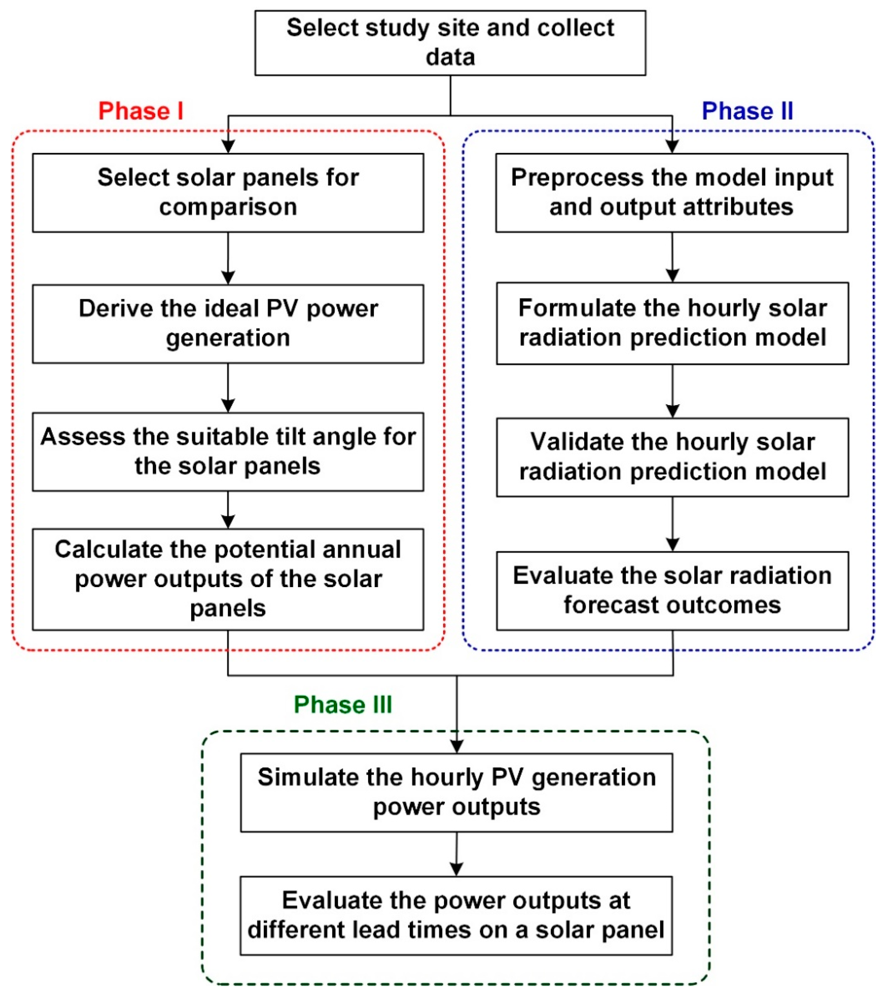
Figure 2 illustrates a flow, which comprises a series of analysis steps. The methodology can be grouped three phases: In phase I, several solar panels were selected for comparison. Solar radiation, module temperature, and power conversion efficiency affect solar cell power output. Therefore, these three parameters were used to derive a formula for ideal PV power generation. Conventional rooftop solar panels can be installed at an inclined angle to maximize the irradiance absorption according to the locations of their installation. Thus, the suitable tilt angle for the PV power generation panels leading to direct sunlight can be achieved to increase power output of the panels installed on building rooftops. Therefore, the potential annual power outputs of these solar panels can be calculated.
In phase II, the surface solar radiation prediction model, which was developed for predicting hourly solar irradiation in the future, was created. First, the model input and output attributes from the ground weather data and solar position parameters are preprocess. A traditional training–validation–testing procedure is adopted for formulating the surface solar radiation prediction model. A DNN is used to create a solar radiation prediction model, and a backpropagation neural network (BPN) and a LR model are implemented as benchmark models. Finally, the testing data set is simulated using the optimal trained model, and the forecast results are evaluated according to the performance measures.
In phase III, the hourly PV power outputs on a solar panel were simulated. The solar radiation prediction model was used to predict the hourly solar radiation, and the hourly amount of power generated by the solar panels was calculated using the process in phase I. Finally, the solar panels were evaluated according to the errors made by the predicted power outputs on various lead times.
3. Selection of Solar Panels
The PV system is a well-recognized system and is widely used to convert the solar energy for electric power generation applications [48]. A cell is defined as a semiconductor device that converts sunlight into electricity. A PV module refers to numerous cells connected in series, and in a PV array, modules are connected in series and in parallel [49]. PV cells represent the fundamental conversion unit of a PV power generation system. Solar insolation, PV cell temperature and operating voltage strongly influence the PV output current and power characteristics [50].
The most critical components of PV power generation systems are PV cells. The quality of these cells directly affects the efficiency and lifetime of a PV system. This study focused on the solar panels manufactured by BP Solar. BP has been involved in solar power since 1973. Its subsidiary, BP Solar, is a manufacturer and installer of photovoltaic solar cells headquartered in Madrid, Spain, with production facilities in United States, Spain, India, China and Australia [51]. The BP3 series solar panel is an advanced PV module that incorporates polycrystalline cells by using SiN coating to provide high efficiency. For evaluation, different BP3 series solar panel types, namely BP350, BP365, BP380, and BP3125, were selected. Table 1 lists the characteristics of the BP3 series solar panels; in particular, BP3125 generated the highest amount of power (125 W).
3.1. Deriving Ideal PV Power Generation
Irradiance is a major factor affecting the amount of solar cell–generated power. The higher the irradiance, the higher the amount of power a solar cell generates. Accordingly, the relationship between irradiance and amount of solar cell–generated power is as follows [52]:
where P indicates the amount of power generated by a solar cell, G indicates the clear-sky global horizontal irradiance (W/m2), A indicates the area of the solar cell (m2), and η indicates the power conversion efficiency (%). The standard environmental parameters for solar panels are G0 = 1000 W/m2 and Tc0 (module temperature of the solar panel) = 25 °C.
P = G × A × η
By using Equation (1), the power conversion efficiency of a solar panel at the module temperature of 25 °C is calculated as follows:
where Pmax indicates the maximal power output by a solar panel module.
Equation (2) yields the η value at the module temperature of 25 °C. Pmax and A0 can be referenced from the characteristic data of the four BP3 series solar panels as listed in Table 1. The value of η for BP350, BP365, BP380, and BP3125 was 11.1%, 11.7%, 12.4%, and 12.3%, respectively.
Higher solar cell module temperature results in lower power generation efficiency. Specifically, for BP3 series solar panels, when the module temperature exceeds 25 °C, each additional 1 °C reduces the overall efficiency by λ = −0.5%/°C. The efficiency change ε in this condition is accordingly expressed as follows:
ε = λ·(Tc − 25)·η
This formula is used to further evaluate the amount of power output after temperature changes:
P = G·A·(η − ε)
Applying Equation (3) to Equation (4) we obtain the following:
P = G·A·[1 − λ·(Tc − 25)]·η
As indicated, the operating cell temperatures of PV modules directly affect the performance of the PV system. Temperature of PV cells is one of the most important parameters for assessing the long term performance of PV module systems and their annual amounts of electrical energy production [53]. Therefore, estimating the operating temperature of a PV module is required. Several mathematical equations for PV module temperature have been found in the literature (e.g., [54,55,56,57,58]). These proposed approaches used empirical formulas to derive the PV cell temperature from the environmental variables, such as ambient temperature, irradiance, and wind speed [5]. A detailed comparison among these empirical formulas was reported by [59,60]. Because Taiwan has an island climate, wind velocity must be factored in. For simplicity, a mathematical model proposed by [61] was employed to account for ambient temperature, irradiance, and wind speed:
where Vw is the wind speed.
Tc = Ta + 0.0138·(1 + 0.031·Ta)(1 − 0.042·Vw)·G
3.2. Equation for Irradiance Received by Inclined Solar Panels
Most available solar radiation data around the world are global solar radiations on a horizontal surface. In practice, solar collectors (flat plate thermal or PV collectors) are tilted; thus, computing the solar radiation incident on such tilted planes is necessary [16]. As calculated in Equation (5), G represents clear-sky global horizontal irradiance. The amount of solar radiation received by solar panels at an inclination must be estimated to accurately calculate their power output.
According to [62], the theoretical global irradiance with the solar panels at a tilted position (Gtilt) can be estimated using the following expression:
where DC is the diffuse horizontal irradiance; IC is the direct irradiance; and Θ the solar incident angle, defined as the angle between the sun and the normal line of the solar panels.
In Equation (7), DC is calculated as follows [63]:
where GC is the clear-sky solar irradiance and θ is the zenith angle.
In Equation (7), the solar incident angle Θ on the inclined solar panel should also be estimated; Θ is expressed according to the latitude of the panel (λ), declination angle (δ), and hour angle (ω) as shown in the following equation:
where β indicates the horizontal inclination angle of the panel.
3.3. Estimating the Power Output of the Inclined Solar Panels
This study focused on the weather station in Tainan (22°99′ N and 120°20′ E). The station is under the jurisdiction by the Central Weather Bureau of Taiwan and records hourly surface climate data, including clear-sky global horizontal irradiance, ambient temperature, and wind velocity. The year 2016 was designated as the simulation year. The hourly clear-sky global horizontal irradiance data recorded in the station were applied in the formulas specified in Section 3.2 to calculate the hourly irradiance received the inclined solar panels. According to [39], the maximal annual global irradiance at Southern Taiwan occurred at β ranging from 20° to 22°. Thus, this study selected β = 21° as the tilt angle of solar panels for the BP3 series.
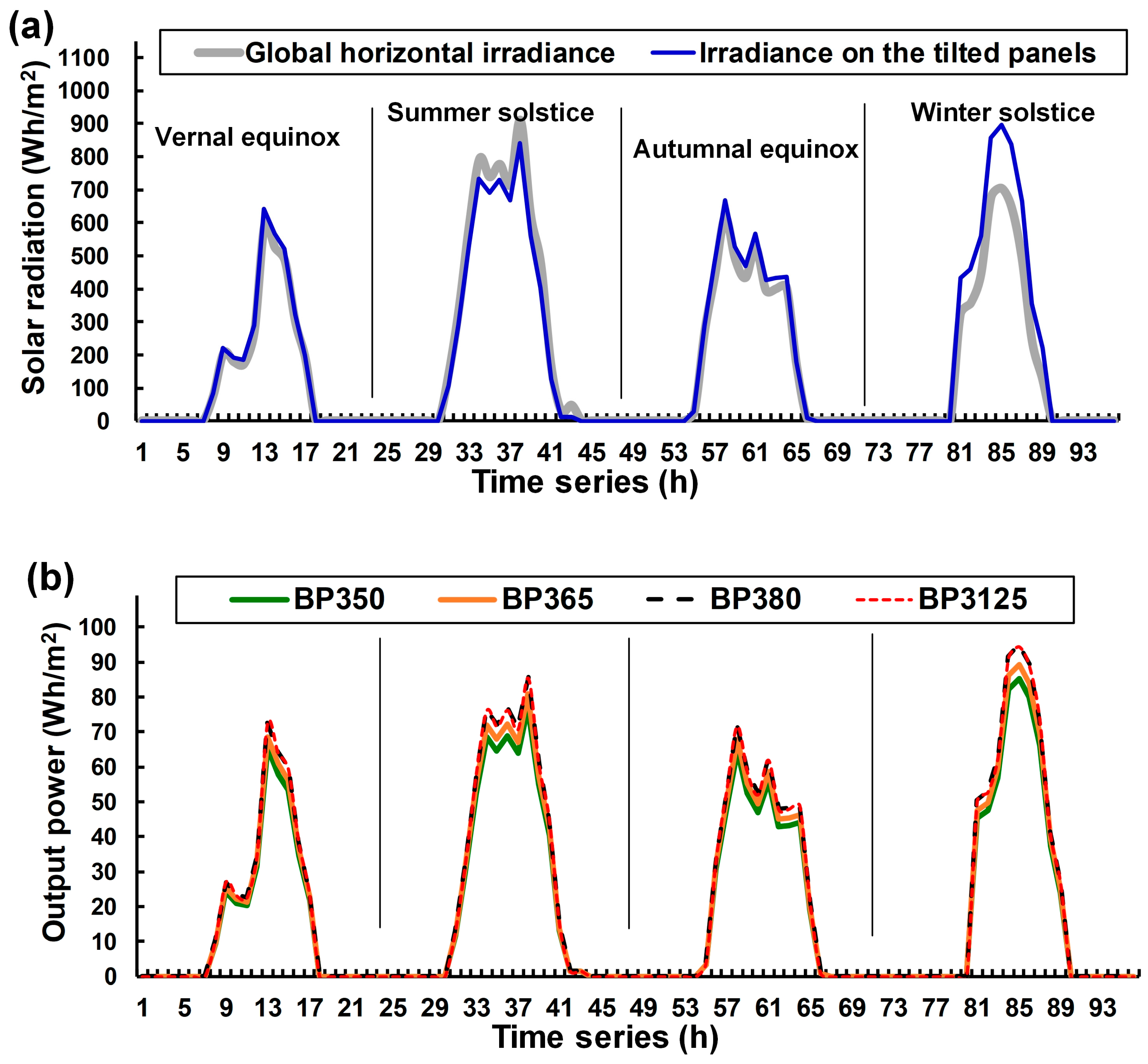
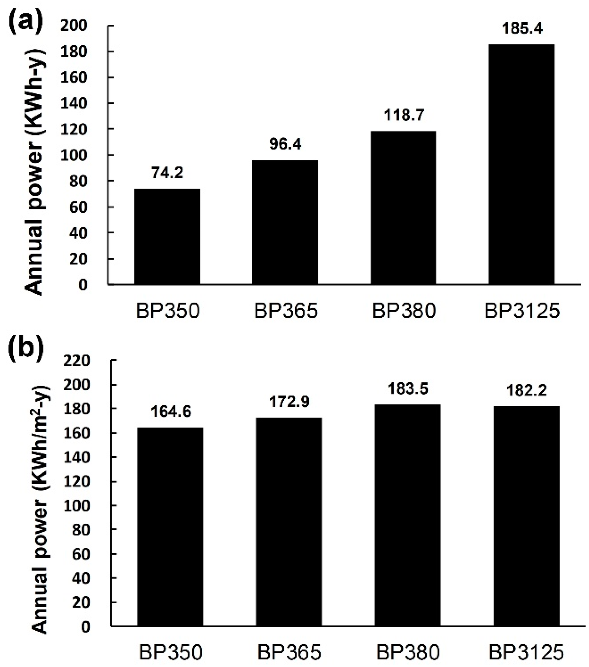
The process of evaluating the selected BP3 series solar panels started with the simulation of hourly irradiance captured by the inclined solar panels. Figure 3a illustrates the simulation results of the hourly solar radiation at the spring and autumn equinoxes and summer and winter solstices in 2016. The formula for the ideal PV power generation was subsequently implemented to estimate the power generated by the solar panels. Figure 3b depicts the power output of the four solar panel modules when β = 21°. Figure 4 illustrates the simulated total power output by the panels in 2016. Figure 4a displays the single module power output; in particular, BP3125 exhibited the highest power generation efficiency (185.4 KWh-y), whereas BP350 was the least efficient module in power generation (74.2 KWh-y). To estimate the PV power output per unit area in a reasonable manner, the power output by each module was divided by the its area to identify its unit area PV power output (Figure 4b). In particular, BP380 exhibited the highest unit area power output (183.5 KWh/m2-y), followed by BP3125 (182.2 KWh/m2-y); BP350 exhibited the lowest unit area power output (164.2 KWh/m2-y).
4. Hourly Solar Radiation Prediction
As indicated by [16], the efficiency or productivity of such a system depends on the temporal fluctuations of energy input and output. Therefore, an hourly solar radiation prediction model was established to further simulate the hourly power output of the solar panels in future for subsequent analysis.
4.1. Experimental Data
Data on surface climate and sun positions were applied in establishing the solar radiation prediction model. In addition to the 2016 data, the 2010–2015 hourly climate data from the weather station were implemented. Seven surface climate parameters related to solar radiation were selected: air pressure on the ground (hPa), ground temperature (°C), relative humidity (%), and surface wind velocity (maximum 10 min mean, 10 m above the surface) (m/s), precipitation within 1 h (mm), sunshine duration (h), and surface solar radiation (Wh/m2); all data were recorded hourly. Sunshine duration, a measure of the time interval for which sunshine is observed in 1 h (at the study location), was used as a climatological indicator of cloudiness. In total, 61,368 data points were organized. Table 2 presents the seven attributes selected and their statistics with mean, standard deviation, maximum, and minimum values; all variables in the database were measured hourly.
Five sun position parameters were selected to illustrate the sun position data relative to the station over time, namely declination, hour, zenith, elevation, and azimuth angles. These parameters are based on the formula proposed by [62,63]. Table 3 lists the statistical data of the hourly sun positions from 2010 to 2016.
4.2. DNNs and Modeling
The solar radiation prediction model was based on a DNN, which is a machine learning model that automatically identifies the representative features through linear or nonlinear transforms in multiple layers. A neural network, which is a mathematical model mimicking the neural system of an organism, features several layers of neurons, which sum the data inputted from the neurons of previous layers and convert them to output data through an activation function. Each neuron is linked to the neurons of the follow-up layer in a unique manner; the data output produced by the neurons from a layer are weighted and transmitted to the neurons of the follow-up layer [64].
DNNs consist of at least one hidden layer. Similar to shallow neural networks, DNNs establish models based on complex nonlinear systems; however, multiple hidden layers are included to enhance the learning efficacy of these models and thereby their prediction and categorization capability. Most DNNs are constructed as feedforward neural networks [65]. DNNs are trained through backpropagation. The weight updates between layers are calculated through stochastic gradient descent:
where wij (t) is the weight set connecting the layers i and j at time t; Δw is the weight correction; η is the learning rate; β is a momentum coefficient; and E is a cost function, which indicates the difference between the target and predicted values. In particular, η and β are hyperparameters for the adjustment of the spacing of weight correction.
In the DNN training process, the weight set in the model can be optimized through a numerical method for minimizing learning target values. This is typically achieved through stochastic gradient descent, in which all weights in high-dimensional spaces descend by one dimension per step; the iteration is repeated multiple times to identify the optimal weight set.
4.3. Modeling and Parameter Calibration
A DNN was used to establish an accurate solar radiation prediction model. The model was established according to the data attributes mentioned in Section 4.1. The employed data were divided into two datasets: 2010–2015 data defined as the training set for model training and verification and 2016 data were designated as the testing set. Model training and verification were performed through 10-fold cross-validation, in which the training set was divided into 10 subsamples, one of which was retained for model verification and the other nine were used for model training; in the verification process, each subsample must be verified.
Building the prediction model requires setting up the neural network structure; in particular, the number of DNN layers, the number of neurons per layer, and the activation function must be defined. Parameter settings affect the efficacy of a DNN model; therefore, an optimized weight set is required for DNN training. Most activation functions are designed for nonlinear transformation for information transfer in a complicated neural network. Conventional activation functions are designed as sigmoid functions or hyperbolic tangent functions. In DNNs, rectified linear unit function has been recently used to replace the sigmoid function, resulting in high performance and short training times, as reported by [66]. Moreover, the number of neurons in the hidden layer was determined according to [67] method: summing numbers of neurons in the input and output layers, subtracting 1 from this sum, and dividing this number by 2.
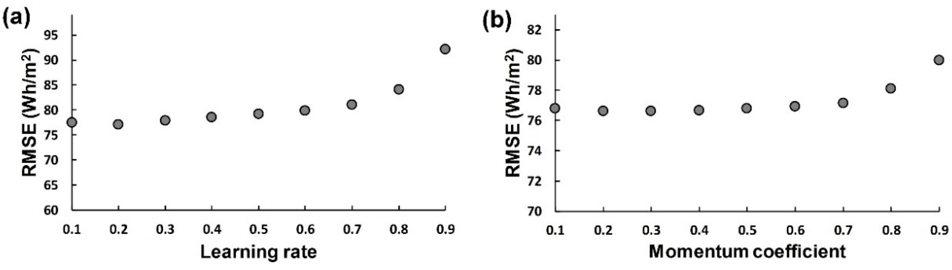
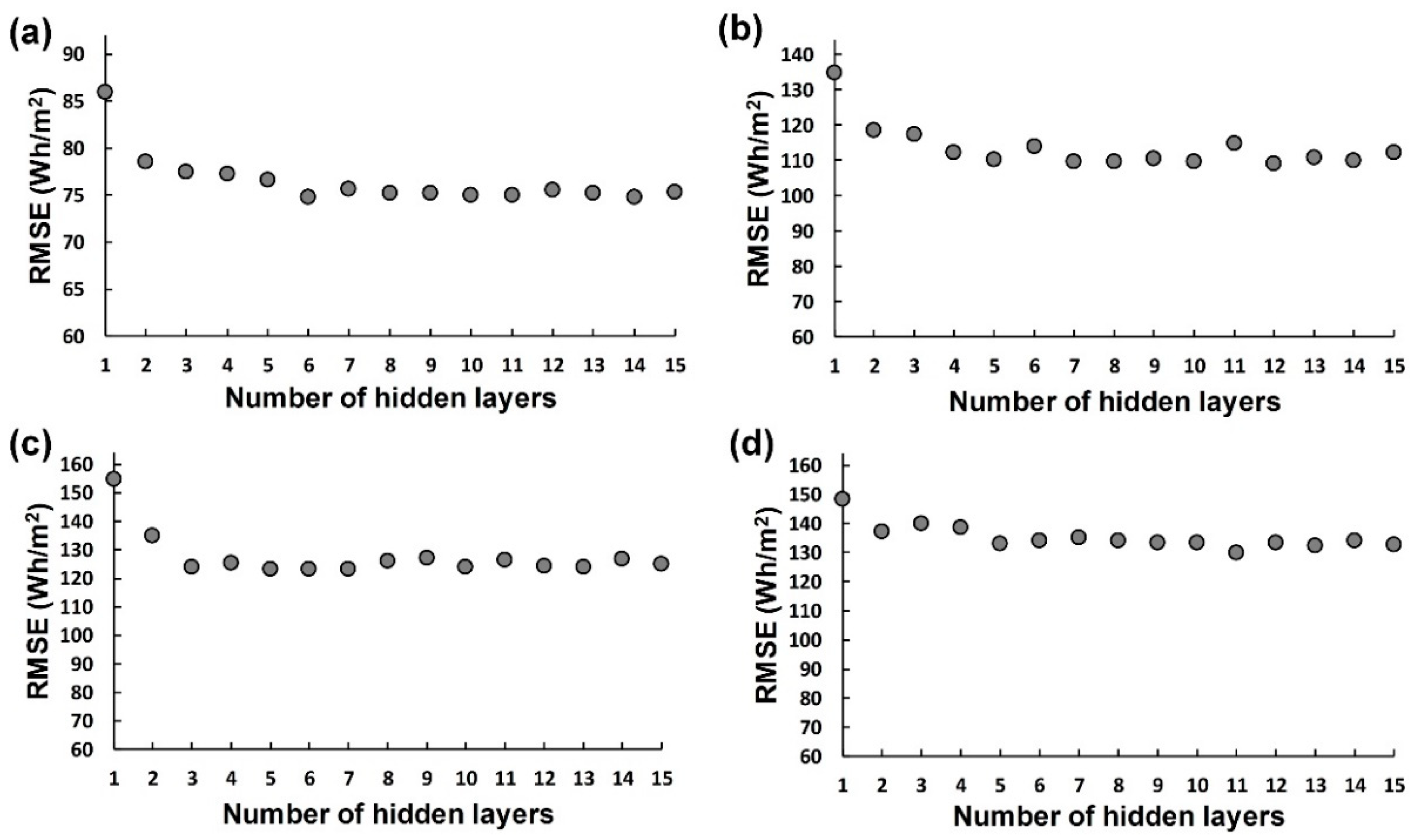
The hyperparameters η and β were verified. Because both parameters range from 0 to 1, intervals of 0.1 were adopted in the verification; subsequently, the root mean square errors (RMSEs) between their output and target values were calculated. Figure 5 illustrates the verification results, in which minimal RMSEs for η and β (77.195 and 76.612 Wh/m2, respectively) were obtained when η = 0.2 and β = 0.2. In addition, the number of DNN layers was determined as 1–15. Figure 6a depicts the RMSEs of the model in the follow-up hour according to the number of layers. When the number of layers was 6, the RMSE decreased (74.846 Wh/m2). Figure 6b–d depicts the RMSEs at lead times of 3, 6, and 12 h, respectively, which were minimized when the numbers of layers were 12, 6, and 11, respectively.
4.4. Forecast of Solar Radiation Prediction
After the model parameters were verified, the testing set was used to predict solar radiation. The simulation results of the DNN model were compared with those of the benchmark models (i.e., BPN and LR models) to verify its quality. A typical BPN, which is a shallow neural network, with three layers (i.e., an input layer, a hidden layer, and an output layer) is a feedforward neural network trained with the standard backpropagation algorithm [68].
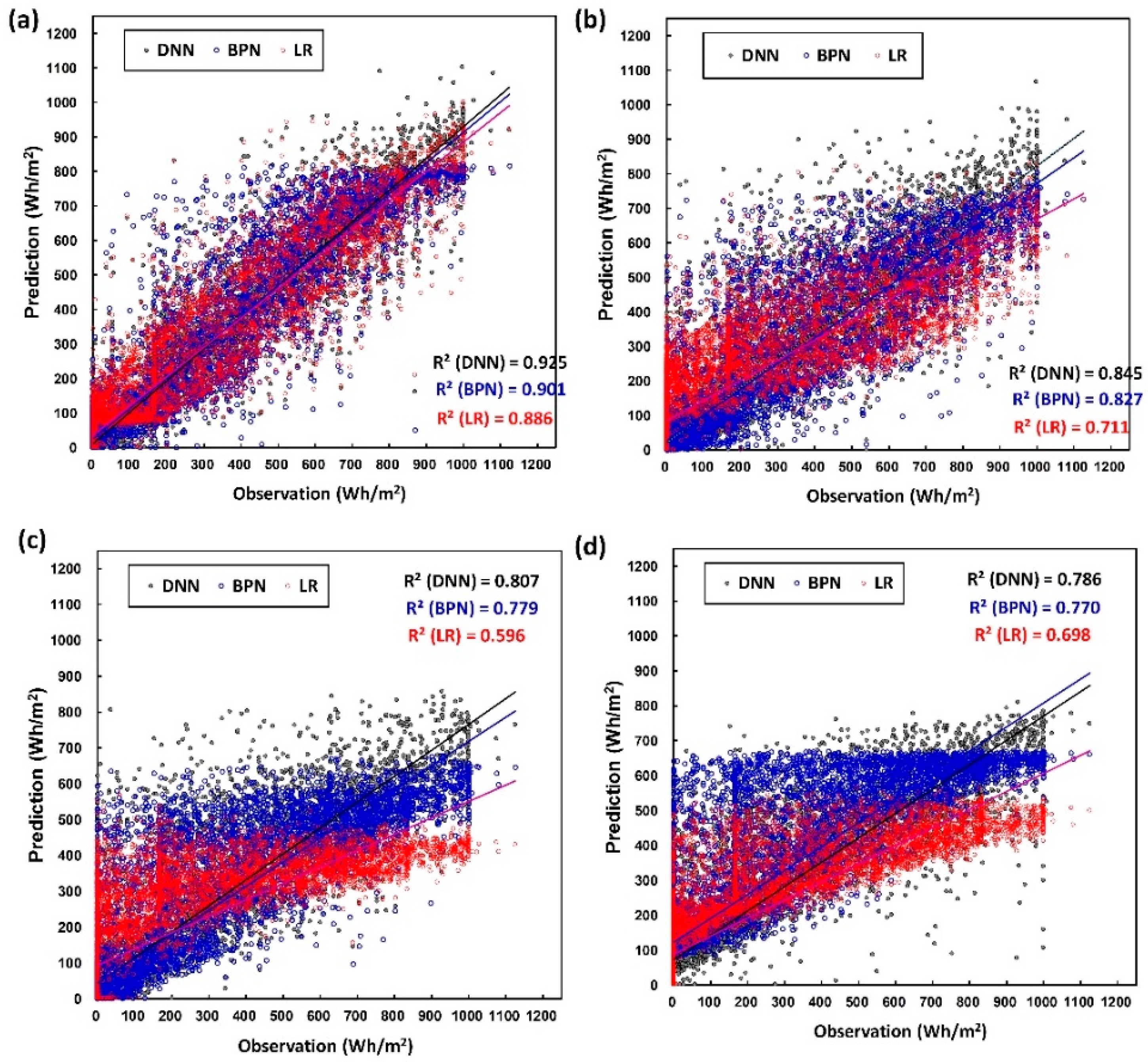
Figure 7 illustrates the scatter diagrams of the predicted and observed values of DNN, BPN, and LR. In particular, Figure 7a–d depict the results at the lead times of 1, 3, 6, and 12 h, respectively. As the lead time increased, the predicted values of DNN became closer to the observed values than did those of BPN and LR. Regarding data correlation, all four figures depicts that DNN exhibited the highest coefficient of determination (R2), followed sequentially by those of BPN and LR.
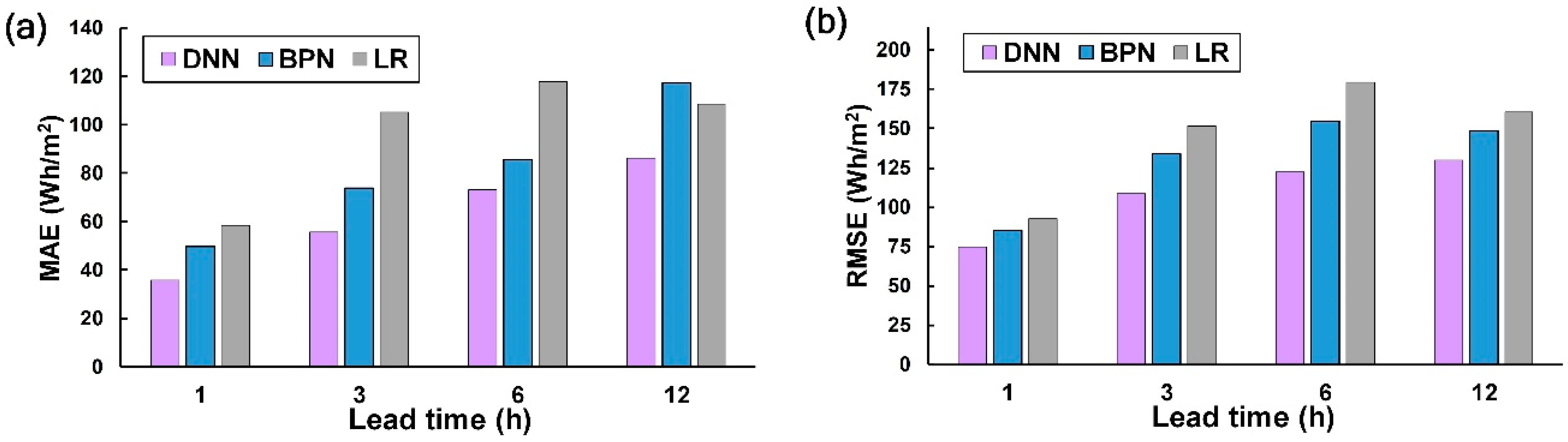
Regarding prediction errors, Figure 8 depicts the calculation results of the three mentioned models. At lead times of 1, 3, 6, and 12 h, DNN exhibited the lowest mean absolute errors (MAEs), indicating that its prediction errors were the lowest overall. Furthermore, DNN displayed the smallest RMSE.
5. Simulation of PV Power Generation
BP3125 was used as the sample solar panel for estimating the PV power output at lead times of 1–12 h. As mentioned previously, after the hourly solar radiation captured by the inclined BP3 series solar panels was simulated using the clear-sky global horizontal irradiance data in 2016, it was used to estimate the hourly power output by the panels (Figure 3). The DNN-based solar radiation prediction model was subsequently employed to replace the predicted values with the observed values to calculate the hourly power output.
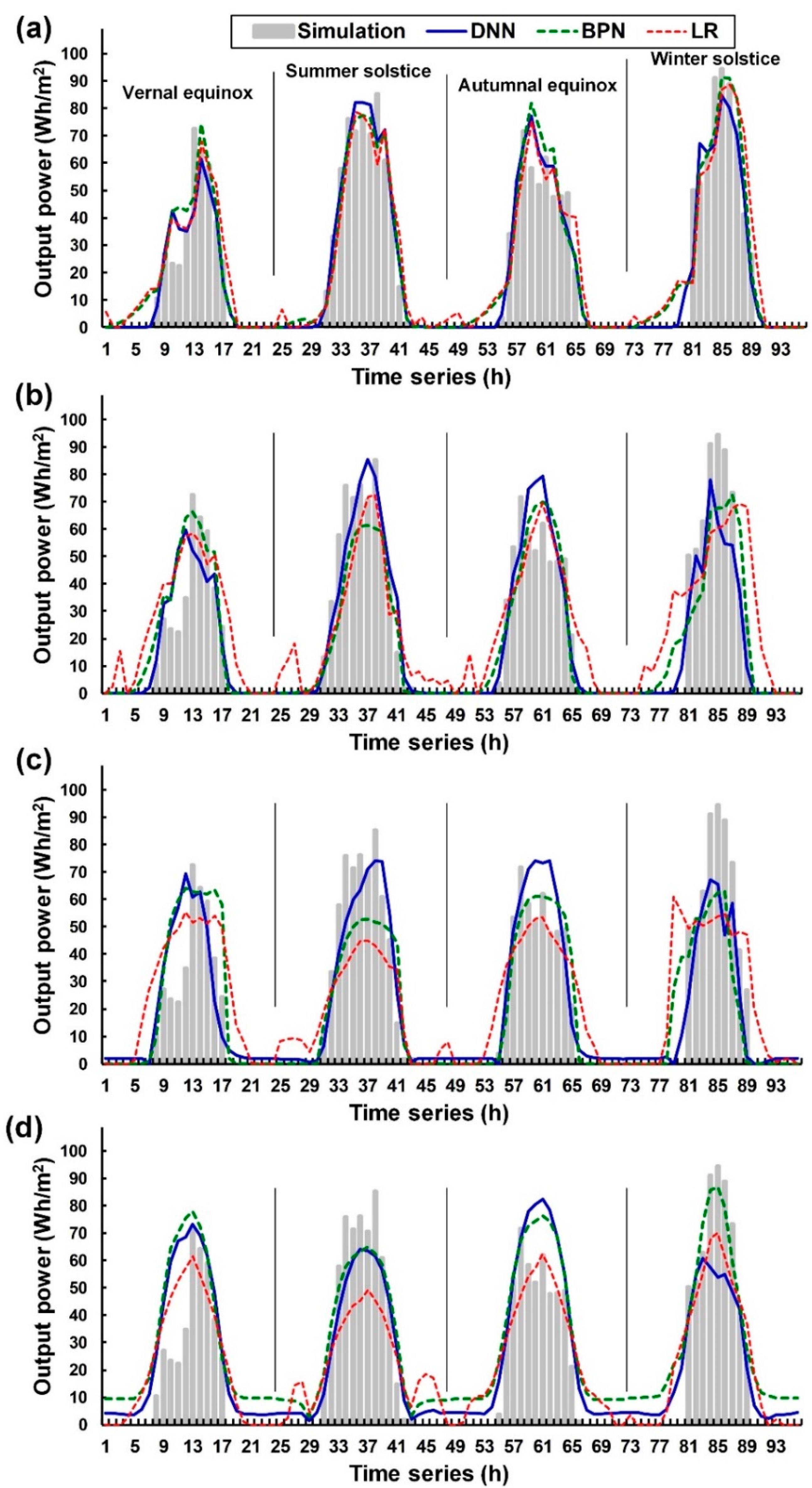
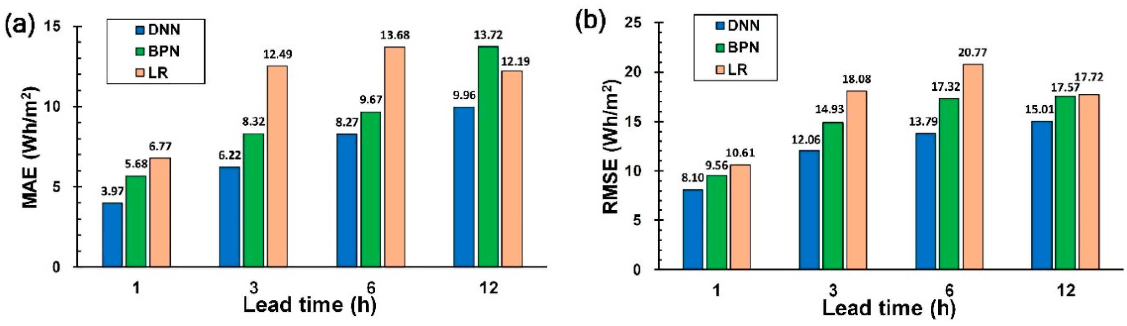
Figure 9 depicts the time sequences of the simulation and predicted values of the power output by BP3125 at the spring and autumn equinoxes and summer and winter solstices in 2016. Figure 9a–d depict the results at the lead times of 1, 3, 6, and 12 h, respectively. The simulation values indicated in Figure 9a represent the simulated power output of BP3125 from Figure 3b; the DNN, BPN, and LR values are the power output values calculated according to the clear-sky global horizontal irradiance estimated through the DNN, BPN, and LR models. Because solar radiation changes substantially each day, the results as depicted in Figure 9 do not represent the daily prediction results in the entire year. Therefore, the evaluation indices for the hourly predicted and simulation values from each model in 2016 were calculated. As shown in Figure 10, DNN exhibited the lowest MAEs and RMSEs at the lead times of 1, 3, 6, and 12 h; this revealed that DNN was the most satisfactory of the three models in predicting solar radiation.
6. Usage and Limitations of the Methodology
In this study, we demonstrated a methodology for developing a usable scheme for evaluating the annual power produced by various solar panels installed on the rooftops of buildings. Tainan, Taiwan, a subtropical region, was used as the experimental site. In practice, the proposed methodology can be used in regions that are suitable for generating and using solar energy. However, the different regions might not have the same climatic conditions as Tainan. Therefore, when using the proposed methodology in such regions, some parameters used in the PV module should be carefully adjusted to suit the local climatic conditions. For instance, when determining the PV cell temperature in these regions, the empirical formulas of PV cell temperature should be reselected because the PV cell temperature is affected by climatic variables, such as irradiance and wind speed.
For examining PV panel brands (e.g., BP Solar), data of the panel manufacturer were obtained. The module products of this brand, such as BP350, BP365, BP380, and BP3125, were assessed for determining their PV output efficiency. When assessing the module products created by different manufacturers, the evaluation process also can be reproduced by the proposed approach. Thus, when the characteristics of the solar panel products are known (i.e., maximum power, voltage and current at maximum power, temperature coefficient of power, and dimension of module), the potential annual power outputs of solar panels can be calculated.
When we developed a surface solar radiation prediction model for PV power generation panels, the solar radiation was estimated by using DNN and BPN, which are data-driven prediction models based on machine learning. A data-driven model is based on the analysis of the data regarding a specific system [69]. Thus, in the modeling process, we used data that were collected from ground-based meteorological stations. However, for regions without ground-based meteorological stations, machine learning-based solar radiation prediction models cannot be developed. Hence, the use of data from satellite measurements is suggested for constructing machine learning-based prediction models in these regions, without ground-based meteorological stations.
7. Conclusions
This study proposed a simple and effective model for evaluating the PV power generation efficiency of each brand of solar panels when planning the installation of rooftop PV systems. Tainan, which has a stable climate and constant sunshine and is suitable for solar power generation in all seasons, was selected as the experimental site. Four BP3 series solar panel types were selected for evaluation: BP350, BP365, BP380, and BP3125.
In phase I, a formula for ideal PV power generation was derived for calculating the power conversion efficiency of each BP series module (11.1%, 11.7%, 12.4%, and 12.3% for BP350, BP365, BP380, and BP3125, respectively). Solar panels are installed at an inclined angle to maximize their reception of solar radiation. Thus, we determined the suitable tilt angle for the PV system leading to direct sunlight that could be acquired to increase power output installed on building rooftop. Subsequently, the potential annual power outputs for these solar panels were calculated. The annual power output of the BP3 series solar panels per unit area was calculated according to the 2016 climate data. The results indicated that BP380 was the most efficient module for annual power output (183.5 KWh/m2), followed by BP3125 (182.2 KWh/m2); BP350 was the least efficient module (164.2 KWh/m2).
In phase II, to simulate hourly PV power generation with regard to meteorological uncertainty, the surface solar radiation prediction model was developed. The model inputs employed the solar position and meteorological information inputs. This study employed the deep learning–based DNN for predicting hourly irradiation. The prediction results of the DNN model were then compared with those of the BPN and LR models. A traditional training–validation–testing procedure was adopted for formulating the surface solar radiation prediction model. The results indicated that the DNN exhibited the lowest MAEs and RMSEs among all three models at the lead times of 1, 3, 6, and 12 h, highlighting its satisfactory prediction accuracy. In phase III, we used the panel of module BP3125 as an example and predicted hourly PV power outputs at different lead times on a solar panel. The evaluation indices for the hourly predicted and simulation values of each model in 2016 were calculated, revealing that DNN exhibited the lowest MAEs and RMSEs among all the three models at the lead times of 1, 3, 6, and 12 h.
The approach proposed in this study was confirmed to be applicable to the evaluation of the power generation efficiency of solar panels and prediction of their hourly power output in an entire year. This approach is suitable for assessing the power generation efficiency of a rooftop PV system.
Author Contributions
C.-C.W. devised the experimental strategy and carried out this experiment and wrote the manuscript and contributed to the revisions.
Funding
This study was supported by the Ministry of Science and Technology, Taiwan, under Grant No. MOST107-2111-M-019-001-CC3. The authors would like to express their sincere appreciation for this grant.
Acknowledgments
The author acknowledges the experimental data provided by the Central Weather Bureau of Taiwan.
Conflicts of Interest
The authors declare no conflict of interest.
References
- Zahedi, A. Solar photovoltaic (PV) energy; latest developments in the building integrated and hybrid PV systems. Renew. Energy 2006, 31, 711–718. [Google Scholar] [CrossRef]
- Messenger, R.; Ventre, J. Photovoltaic Systems Engineering; CRC Press: Boca Raton, FL, USA, 2000; pp. 11–12, 41–51. [Google Scholar]
- Chen, F.C. A Meteorology Assessment for Photovoltaic Generation. Master’s Thesis, Southern Taiwan University of Science and Technology, Tainan, China, 2006. (In Chinese). [Google Scholar]
- Sopian, K.; Cheow, S.L.; Zaidi, S.H. An overview of crystalline silicon solar cell technology: Past, present, and future. AIP Conf. Proc. 2017, 1877, 020004. [Google Scholar]
- Muzathik, A.M. Photovoltaic modules operating temperature estimation using a simple correlation. Int. J. Energy Eng. 2014, 4, 151–158. [Google Scholar]
- Kim, B.C.; Kim, J.; Kim, K. Evaluation model for investment in solar photovoltaic power generation using fuzzy analytic hierarchy process. Sustainability 2019, 11, 2905. [Google Scholar] [CrossRef]
- Kovač, M.; Stegnar, G.; Al-Mansour, F.; Merše, S.; Pečjak, A. Assessing solar potential and battery instalment for self-sufficient buildings with simplified model. Energy 2019, 173, 1182–1195. [Google Scholar] [CrossRef]
- Le, N.T.; Benjapolakul, W. Evaluation of contribution of PV array and inverter configurations to rooftop PV system energy yield using machine learning techniques. Energies 2019, 12, 3158. [Google Scholar] [CrossRef]
- Jeong, K.; Hong, T.; Koo, C.; Oh, J.; Lee, M.; Kim, J. A prototype design and development of the smart photovoltaic system blind considering the photovoltaic panel, tracking system, and monitoring system. Appl. Sci. 2017, 7, 1077. [Google Scholar] [CrossRef]
- Mahmud, M.A.P.; Huda, N.; Farjana, S.H.; Lang, C. Environmental impacts of solar-photovoltaic and solar-thermal systems with life-cycle assessment. Energies 2018, 11, 2346. [Google Scholar] [CrossRef]
- Kouhestani, F.M.; Byrne, J.; Johnson, D.; Spencer, L.; Hazendonk, P.; Brown, B. Evaluating solar energy technical and economic potential on rooftops in an urban setting: The city of Lethbridge, Canada. Int. J. Energy Environ. Eng. 2019, 10, 13–32. [Google Scholar] [CrossRef]
- Balo, F.; Şağbanşua, L. The selection of the best solar panel for the photovoltaic system design by using AHP. Energy Procedia 2016, 100, 50–53. [Google Scholar] [CrossRef]
- Nfaoui, M.; El-Hami, K. Extracting the maximum energy from solar panels. Energy Rep. 2018, 4, 536–545. [Google Scholar] [CrossRef]
- Wang, T.C.; Tsai, S.Y. Solar panel supplier selection for the photovoltaic system design by using fuzzy multi-criteria decision making (MCDM) approaches. Energies 2018, 11, 1989. [Google Scholar] [CrossRef]
- Guechi, A.; Chegaar, M. Effects of diffuse spectral illumination on microcrystalline solar cells. J. Electron Devices Soc. 2007, 5, 116–121. [Google Scholar]
- Notton, G.; Cristofari, C.; Muselli, M.; Poggi, P. Calculation on an hourly basis of solar diffuse irradiations from global data for horizontal surfaces in Ajaccio. Energy Convers. Manag. 2004, 45, 2849–2866. [Google Scholar] [CrossRef]
- Gopinathan, K.K. Solar radiation on variously oriented sloping surfaces. Sol. Energy 1991, 47, 173–179. [Google Scholar] [CrossRef]
- Kambezidis, H.D.; Psiloglou, B.E.; Synodinou, B.M. Comparison between measurements and models for daily solar irradiation on tilted surfaces in Athens, Greece. Renew. Energy 1997, 10, 505–518. [Google Scholar] [CrossRef]
- Robledo, L.; Soler, A. Modelling daylight on inclined surfaces for applications to daylight conscious architecture. Renew. Energy 1997, 11, 149–152. [Google Scholar] [CrossRef]
- Nijmeh, S.; Mamlook, R. Testing of two models for computing global solar radiation on tilted surfaces. Renew. Energy 2000, 20, 75–81. [Google Scholar] [CrossRef]
- Maleki, S.A.M.; Hizam, H.; Gomes, C. Estimation of hourly, daily and monthly global solar radiation on inclined surfaces: Models re-visited. Energies 2017, 10, 134. [Google Scholar] [CrossRef]
- Chen, S.X.; Gooi, H.B.; Wang, M.Q. Solar radiation forecast based on fuzzy logic and neural networks. Renew. Energy 2013, 60, 195–201. [Google Scholar] [CrossRef]
- Ding, M.; Wang, L.; Bi, R. An ANN-based approach for forecasting the power output of photovoltaic system. Procedia Environ. Sci. 2011, 11 Pt C, 1308–1315. [Google Scholar] [CrossRef]
- Dorvlo, A.S.S.; Jervaseb, J.; Al-Lawatib, A. Solar radiation estimation using artificial neural networks. Appl. Energy 2015, 71, 307–319. [Google Scholar] [CrossRef]
- Inman, R.H.; Pedro, H.T.C.; Coimbra, C.F.M. Solar forecasting methods for renewable energy integration. Prog. Energy Combust. Sci. 2013, 39, 535–576. [Google Scholar] [CrossRef]
- Khandakar, A.; Chowdhury, M.E.H.; Kazi, M.K.; Benhmed, K.; Touati, F.; Al-Hitmi, M.; Gonzales, S.P., Jr. Machine learning based photovoltaics (PV) power prediction using different environmental parameters of Qatar. Energies 2019, 12, 2782. [Google Scholar] [CrossRef]
- Li, Z.; Rahman, S.M.; Vega, R.; Dong, B. A hierarchical approach using machine learning methods in solar photovoltaic energy production forecasting. Energies 2016, 9, 55. [Google Scholar] [CrossRef]
- Monteiro, C.; Santos, T.; Fernandez-Jimenez, L.A.; Ramirez-Rosado, I.J.; Terreros-Olarte, M.S. Short-term power forecasting model for photovoltaic plants based on historical similarity. Energies 2013, 6, 2624–2643. [Google Scholar] [CrossRef]
- Notton, G.; Paoli, C.; Diaf, S. Estimation of tilted solar irradiation using Artificial Neural Networks. Energy Procedia 2013, 42, 33–42. [Google Scholar] [CrossRef]
- Persson, C.; Bacher, P.; Shiga, T.; Madsen, H. Multi-site solar power forecasting using gradient boosted regression trees. Sol. Energy 2017, 150, 423–436. [Google Scholar] [CrossRef]
- Reda, I.; Andreas, A. Solar position algorithm for solar radiation applications. Sol. Energy 2004, 76, 577–589. [Google Scholar] [CrossRef]
- Shen, C.; He, Y.L.; Liu, Y.W.; Tao, W.Q. Modelling and simulation of solar radiation data processing with Simulink. Simul. Model. Pract. Theory 2008, 16, 721–735. [Google Scholar] [CrossRef]
- Yang, D.; Gu, C.; Dong, Z.; Jirutitijaroen, P.; Chen, N.; Walsh, W.M. Solar irradiance forecasting using spatial-temporal covariance structures and time-forward kriging. Renew. Energy 2013, 60, 235–245. [Google Scholar] [CrossRef]
- Yeom, J.M.; Han, K.S. Improved estimation of surface solar insolation using a neural network and MTSAT-1R data. Comput. Geosci. 2010, 36, 590–597. [Google Scholar] [CrossRef]
- Hocaoglu, F.O. Stochastic approach for daily solar radiation modeling. Sol. Energy 2011, 85, 278–287. [Google Scholar] [CrossRef]
- Pedro, H.T.C.; Coimbra, C.F.M. Nearest-neighbor methodology for prediction of intra-hour global horizontal and direct normal irradiances. Renew. Energy 2015, 80, 770–782. [Google Scholar] [CrossRef]
- Bosch, J.L.; Lopez, G.; Batlles, F.J. Daily solar irradiation estimation over a mountainous area using artificial neural network. Renew. Energy 2008, 33, 1622–1628. [Google Scholar] [CrossRef]
- Wang, F.; Mi, Z.; Su, S.; Zhao, H. Short-term solar irradiance forecasting model based on artificial neural network using statistical feature parameters. Energies 2012, 5, 1355–1370. [Google Scholar] [CrossRef]
- Wei, C.C. Predictions of surface solar radiation on tilted solar panels using machine learning models: Case study of Tainan City, Taiwan. Energies 2017, 10, 1660. [Google Scholar] [CrossRef]
- Zhu, H.; Li, X.; Sun, Q.; Nie, L.; Yao, J.; Zhao, G. A power prediction method for photovoltaic power plant based on wavelet decomposition and artificial neural networks. Energies 2016, 9, 11. [Google Scholar] [CrossRef]
- Cao, J.; Lin, X. Application of the diagonal recurrent wavelet neural network to solar irradiation forecast assisted with fuzzy technique. Eng. Appl. Artif. Intell. 2008, 21, 1255–1263. [Google Scholar] [CrossRef]
- Urraca, R.; Antonanzas, J.; Alia-Martinez, M.; Martinez-de-Pison, F.J.; Antonanzas-Torres, F. Smart baseline models for solar irradiation forecasting. Energy Convers. Manag. 2016, 108, 539–548. [Google Scholar] [CrossRef]
- Yousif, J.H.; Kazem, H.A.; Boland, J. Predictive models for photovoltaic electricity production in hot weather conditions. Energies 2017, 10, 971. [Google Scholar] [CrossRef]
- Hinton, G.E.; Osindero, S.; Teh, Y.W. A fast learning algorithm for deep belief nets. Neural Comput. 2014, 18, 1527–1554. [Google Scholar] [CrossRef] [PubMed]
- Ghimire, S.; Deo, R.C.; Raj, N.; Mi, J. Deep learning neural networks trained with MODIS satellite-derived predictors for long-term global solar radiation prediction. Energies 2019, 12, 2407. [Google Scholar] [CrossRef]
- Li, C.; Ding, Z.; Zhao, D.; Yi, J.; Zhang, G. Building energy consumption prediction: An extreme deep learning approach. Energies 2017, 10, 1525. [Google Scholar] [CrossRef]
- Ryu, S.; Noh, J.; Kim, H. Deep neural network based demand side short term load forecasting. Energies 2017, 10, 3. [Google Scholar] [CrossRef]
- Tsai, H.L. Insolation-oriented model of photovoltaic module using Matlab/Simulink. Sol. Energy 2010, 84, 1318–1326. [Google Scholar] [CrossRef]
- Tian, H.; Mancilla-David, F.; Ellis, K.; Muljadi, E.; Jenkins, P. A cell-to-module-to-array detailed model for photovoltaic panels. Sol. Energy 2012, 86, 2695–2706. [Google Scholar] [CrossRef]
- Angrist, S.W. Direct Energy Conversion, 4th ed.; Allyn and Bacon, Inc.: Boston, MA, USA, 1982; pp. 177–227. [Google Scholar]
- BP Official Website. Available online: https://www.bp.com/ (accessed on 10 July 2019).
- Shih, H. Cost and Benefit Analysis of Community-based Solar Power System. Master’s Thesis, National Chiao Tung University, Taiwan, China, 2009. (In Chinese). [Google Scholar]
- Piyatida, T.; Chumnong, S.; Dhirayut, C. Estimating operating cell temperature of BIPV modules in Thailand. Renew. Energy 2009, 4, 2515–2523. [Google Scholar]
- Rauschenbach, H.S. Solar Cell Array Design Handbook; Van Nostrand Reinhold: New York, NY, USA, 1980; pp. 390–391. [Google Scholar]
- Ross, R.G. Interface Design Considerations for Terrestrial Solar Cells Modules. In Proceedings of the 12th IEEE Photovoltaic Specialist’s Conference, Baton Rouge, LA, USA, 7–10 January 1976; pp. 801–806. [Google Scholar]
- Risser, V.V.; Fuentes, M.K. Linear Regression Analysis of Flat-plate Photovoltaic System Performance Data. In Proceedings of the 5th Photovoltaic Solar Energy Conference, Athens, Greece, 17–21 October 1983. [Google Scholar]
- Schott, T. Operation Temperatures of PV Modules: A Theoretical and Experimental Spproach. In Proceedings of the Sixth EC Photovoltaic Solar Energy Conference, London, UK, 15–19 April 1985. [Google Scholar]
- Koehl, M.; Heck, M.; Wiesmeier, S.; Wirth, J. Modeling of the nominal operating cell temperature based on outdoor weathering. Sol. Energy Mater. Sol. Cells 2011, 95, 1638–1646. [Google Scholar] [CrossRef]
- Jakhrani, A.Q.; Othman, A.K.; Rigit, A.R.H.; Samo, S.R. Comparison of solar photovoltaic module temperature models. World Appl. Sci. J. 2011, 14, 01–08. [Google Scholar]
- Kamuyu, W.C.L.; Lim, J.R.; Won, C.S.; Ahn, H.K. Prediction model of photovoltaic module temperature for power performance of floating PVs. Energies 2018, 11, 447. [Google Scholar] [CrossRef]
- Servant, J.M. Calculation of the Cell Temperature for Photovoltaic Modules from Climatic Data. In Proceedings of the 9th biennial congress of ISES- Intersol 85, Montreal, QC, Canada; 1985; p. 370. [Google Scholar]
- Exell, R.H.B. A mathematical model for solar radiation in South-East Asia (Thailand). Sol. Energy 1981, 26, 161–168. [Google Scholar] [CrossRef]
- Markvart, T. Solar Electricity; John Wiley & Sons Ltd.: New York, NY, USA, 1994. [Google Scholar]
- Lo, D.C.; Wei, C.C.; Tsai, N.P. Parameter automatic calibration approach for neural-network-based cyclonic precipitation forecast models. Water 2015, 7, 3963–3977. [Google Scholar] [CrossRef]
- Wei, C.C.; Hsieh, C.J. Using adjacent buoy information to predict wave heights of typhoons offshore of northeastern Taiwan. Water 2018, 10, 1800. [Google Scholar] [CrossRef]
- Nair, V.; Hinton, G. Rectified Linear Units Improve Restricted Boltzmann machines. In Proceedings of the 27th International Conference on Machine Learning, Haifa, Israel; 2010; pp. 807–814. [Google Scholar]
- Trenn, S. Multilayer perceptrons: Approximation order and necessary number of hidden units. IEEE Trans. Neural Netw. 2008, 19, 836–844. [Google Scholar] [CrossRef] [PubMed]
- Tsai, C.C.; Lu, M.C.; Wei, C.C. Decision tree-based classifier combined with neural-based predictor for water-stage forecasts in a river basin during typhoons: A case study in Taiwan. Environ. Eng. Sci. 2012, 29, 108–116. [Google Scholar] [CrossRef]
- Solomatine, D.P.; Ostfeld, A. Data-driven modelling: Some past experiences and new approaches. J. Hydroinform. 2008, 10, 3–22. [Google Scholar] [CrossRef]
Figure 1.
Map of Tainan, Taiwan.

Figure 2.
Flow of evaluation of power outputs of a solar panel.

Figure 3.
Spring and autumn equinoxes and summer and winter solstices in 2016: (a) Hourly solar radiation; (b) Estimated hourly output power of BP3 series modules.
Figure 3.
Spring and autumn equinoxes and summer and winter solstices in 2016: (a) Hourly solar radiation; (b) Estimated hourly output power of BP3 series modules.

Figure 4.
Simulated annual power output by the BP3 series: (a) Single module; (b) Unit area.

Figure 5.
Calibration of hyperparameters: (a) Learning rate; (b) Momentum coefficient.

Figure 6.
Calibration of hidden layer amount at lead times of (a) 1; (b) 3; (c) 6 and (d) 12 h.

Figure 7.
Scatter diagram of deep neural network (DNN), backpropagation neural network (BPN) and linear regression (LR) at the lead times of (a) 1; (b) 3; (c) 6 and (d) 12 h.
Figure 7.
Scatter diagram of deep neural network (DNN), backpropagation neural network (BPN) and linear regression (LR) at the lead times of (a) 1; (b) 3; (c) 6 and (d) 12 h.

Figure 8.
Solar radiation prediction performance: (a) mean absolute error (MAE) and (b) root mean square error (RMSE).
Figure 8.
Solar radiation prediction performance: (a) mean absolute error (MAE) and (b) root mean square error (RMSE).

Figure 9.
Simulation and predicted values on the hourly power output of BP3125 at spring and autumn equinoxes and summer and winter solstices in 2016 at lead times of (a) 1; (b) 3; (c) 6 and (d) 12 h.
Figure 9.
Simulation and predicted values on the hourly power output of BP3125 at spring and autumn equinoxes and summer and winter solstices in 2016 at lead times of (a) 1; (b) 3; (c) 6 and (d) 12 h.

Figure 10.
Annual performance of predicted power outputs of module BP3125: (a) MAE and (b) RMSE.


Table 1.
Characteristics of BP3 series solar panel products.
| Module | Maximum Power (Pmax) | Voltage at Pmax | Current at Pmax | Temperature Coefficient of Power | Dimension of Module |
|---|---|---|---|---|---|
| BP350 | 50 W | 17.3 V | 2.89 A | −0.5%/°C | 839 mm × 537 mm |
| BP365 | 65 W | 17.6 V | 3.69 A | −0.5%/°C | 1111 mm × 502 mm |
| BP380 | 80 W | 17.6 V | 4.55 A | −0.5%/°C | 1204 mm × 537 mm |
| BP3125 | 125 W | 17.6 V | 7.1 A | −0.5%/°C | 1510 mm × 674 mm |
Table 2.
Weather attributes and statistics at the Tainan station.
| Attribute | Air Pressure on the Ground | Ground Temperature | Relative Humidity | Surface Wind Velocity | Precipitation | Sunshine Duration | Surface Solar Radiation |
|---|---|---|---|---|---|---|---|
| Unit | hPa | °C | % | m/s | mm | h | Wh/m2 |
| Mean | 1009.8 | 24.60 | 74.38 | 2.97 | 0.21 | 0.23 | 188.87 |
| Std. dev. | 5.663 | 5.234 | 10.34 | 1.689 | 1.829 | 0.37 | 276.52 |
| Maximum | 1029.6 | 35.8 | 100 | 19.5 | 90.5 | 1 | 1161.1 |
| Minimum | 973.4 | 5.8 | 22 | 0 | 0 | 0 | 0 |
Table 3.
Solar position attributes and statistics at the Tainan station.
| Title Attribute | Declination Angle | Hour Angle | Zenith Angle | Elevation Angle | Azimuth Angle |
|---|---|---|---|---|---|
| Unit | Degree | Degree | degree | Degree | degree |
| Mean | −0.01 | 7.50 | 90 | 0 | 0 |
| Std. dev. | 16.58 | 103.83 | 43.84 | 43.84 | 65.10 |
| Maximum | 23.45 | 180 | 179.98 | 89.98 | 90.00 |
| Minimum | −23.45 | −165 | 0.02 | −89.98 | −90.00 |
© 2019 by the author. Licensee MDPI, Basel, Switzerland. This article is an open access article distributed under the terms and conditions of the Creative Commons Attribution (CC BY) license (http://creativecommons.org/licenses/by/4.0/).
Share and Cite
MDPI and ACS Style
Wei, C.-C. Evaluation of Photovoltaic Power Generation by Using Deep Learning in Solar Panels Installed in Buildings. Energies 2019, 12, 3564. https://0-doi-org.brum.beds.ac.uk/10.3390/en12183564
AMA Style
Wei C-C. Evaluation of Photovoltaic Power Generation by Using Deep Learning in Solar Panels Installed in Buildings. Energies. 2019; 12(18):3564. https://0-doi-org.brum.beds.ac.uk/10.3390/en12183564
Chicago/Turabian StyleWei, Chih-Chiang. 2019. "Evaluation of Photovoltaic Power Generation by Using Deep Learning in Solar Panels Installed in Buildings" Energies 12, no. 18: 3564. https://0-doi-org.brum.beds.ac.uk/10.3390/en12183564
Note that from the first issue of 2016, this journal uses article numbers instead of page numbers. See further details here.