Partial Discharge Data Matching Method for GIS Case-Based Reasoning
by
 ,
,
Jiejie Dai
1,* ,
,
Yingbing Teng
1,
Zhaoqi Zhang
2,
Zhongmin Yu
3,
Gehao Sheng
2 and
Xiuchen Jiang
2 1
State Grid Shanghai Shinan Electric Power Supply Company, Xinbei Road No.268, Shanghai 201199, China
2
Department of Electrical Engineering, Shanghai Jiao Tong University, Dongchuan Road No.800, Shanghai 200240, China
3
State Grid Shanghai Electric Power Company, Yuanshen Road No.1122, Shanghai 200120, China
*
Author to whom correspondence should be addressed.
Energies 2019, 12(19), 3677; https://0-doi-org.brum.beds.ac.uk/10.3390/en12193677
Submission received: 6 August 2019
/
Revised: 10 September 2019
/
Accepted: 24 September 2019
/
Published: 26 September 2019
(This article belongs to the Special Issue Data Mining in Smart Grids)
Abstract
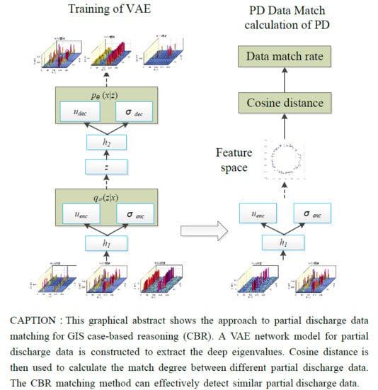
:With the accumulation of partial discharge (PD) detection data from substation, case-based reasoning (CBR), which computes the match degree between detected PD data and historical case data provides new ideas for the interpretation and evaluation of partial discharge data. Aiming at the problem of partial discharge data matching, this paper proposes a data matching method based on a variational autoencoder (VAE). A VAE network model for partial discharge data is constructed to extract the deep eigenvalues. Cosine distance is then used to calculate the match degree between different partial discharge data. To verify the advantages of the proposed method, a partial discharge dataset was established through a partial discharge experiment and live detections on substation site. The proposed method was compared with other feature extraction methods and matching methods including statistical features, deep belief networks (DBN), deep convolutional neural networks (CNN), Euclidean distances, and correlation coefficients. The experimental results show that the cosine distance match degree based on the VAE feature vector can effectively detect similar partial discharge data compared with other data matching methods.
1. Introduction
CIGRE’s statistics show that about 30% dielectric failures of gas insulated switchgears (GIS) are related to design deficiencies [1]. Through the analysis of a large amount of partial discharge (PD) data from GIS in service, we also found that the proportion of PD cases caused by design reasons is high. This leads to a situation that the same type GIS equipment from the same manufacturer are susceptible to repeat partial discharge on similar location. This provides the basis for case-based reasoning (CBR) in GIS. Case-based reasoning is a branch of artificial intelligence (AI) that provides answers to new questions based on experience in historical cases [2,3]. In the latest studies, CBR has been used in load forecasting, energy management, grid system safety assessment, and power equipment failure assessment [4,5,6,7]. In Reference [8], a case-based reasoning method is utilized to diagnose the incipient fault of power transformer. Pretreated dissolved gas analysis (DGA) data is used in the CBR system. Reference [9] developed a case-based reasoning approach for identifying and filtering acoustic emission (AE) noise signals. The paper proposed a parametric case representation method for the AE signal process. Since CBR requires the accumulation of cases and data in the early stage, there is no CBR related literature published in the field of partial discharge. After accumulating a large amount of GIS PD detection data from substation site, CBR can provide new ideas for the interpretation and evaluation of partial discharge data. The key step in a CBR system is the case matching strategy. PD data is one of the key features in a GIS PD detection case. So this paper focused on the data matching problem in the CBR system establishment. A structure of GIS, CBR used PD data, the match degree is presented and shown in Figure 1.
Some phase resolved pulse sequence (PRPS) graphs are used in Figure 1 to refer to the data detected by the GIS partial discharge ultra-high frequency (UHF) detection. The specific procedures are as follows: First, the historical data are retrieved from the historical case database according to the operating conditions of the detected equipment, the manufacturer and other search conditions; the detected data are then matched with the historical data, and those cases for which the data match degree exceeds a threshold are considered match cases; and finally, from the match case, we can obtain information such as the highest probability of PD location in the detected power equipment, the most likely cause of PD in the detected power equipment, and pictures of disintegrated power equipment in historical cases. Maintenance plans can be developed based on match information. Therefore, PD history detection data can be more effectively utilized and can provide a basis for data-driven device status evaluations.
There are two key processes that are used to calculate PD data match degree. The first key process is to extract the valid eigenvalues for PD data, and the second is to obtain the match degree (MD) based on the eigenvectors. The traditional feature extraction methods used for PD data extract a variety of statistical features from, for example, histograms, scatter plots, and grayscale images based on PRPD (phase resolved partial discharge) data [10,11,12]. Moreover, there are also some other algorithms applied to PD data feature extraction, such as principal component analysis (PCA) [13], wavelet packets transformation [14], sparse representation [15], and signal norms [16]. The algorithms proposed in the references behaved a good performance in the task of PD pattern recognition. However, due to the multi-source heterogeneity of access data in big data centers, the huge differences in the performances of PD detect instruments and the complex operating environments in substations, the statistical characteristics obtained by the traditional statistical methods have become inadequate in identifications of typical partial discharge types. In addition, data matching of PD data needs even more stringent requirements than those for PD pattern recognition.
In recent years, related technologies such as deep auto-encoders, deep convolutional networks, recurrent neural networks, and deep belief networks have shown good performance in many fields, including image processing and speech processing [17,18,19,20,21]. Reference [22] studied the application of deep neural networks in the diagnosis of partial discharges and demonstrated the improvements in accuracy and visualization that can be obtained through the deep learning method. Reference [23] obtained a two-dimensional spectral frame representation of a UHF signal employing a time-frequency analysis and then used a deep convolutional network to obtain enhanced features under different PD sources. Auto-encoding (AE) is an unsupervised feature learning method, and its hidden layer can effectively extract the internal expression of data. Its deep structure makes the network closer to the human brain’s information hierarchical processing, with better nonlinear modelling ability [24,25]. The variational autoencoder (VAE) proposed by Kingma et al. is a generating network based on variational Bayesian inference [26]. It avoids the computational complexity of dataset likelihood probability calculations and traditional Monte Carlo sampling and is therefore becoming an area of considerable research interest in text classification, semi-supervised learning, and other related fields.
This paper presents a PD data matching method based on VAE. The network uses variational Bayesian method to quickly approximate the posterior probability and extract the deep features of PD data. Euclidean distance, cosine distance, and correlation coefficient (Cc) methods were used to measure the similarity between different data, the comparative results of which are also shown in this paper.
The rest of the paper is organized as follows. Section 2 introduces basic information on variational autoencoder networks. Section 3 provides further information on the proposed partial discharge data matching approach. The dataset used in this paper is described in Section 4. Section 5 validates the data matching approach with different case studies and discusses the results obtained. The conclusions are presented in Section 6.
2. Variational Autoencoder
Variational Bayes inference [27] is a deterministic approximation method that maximizes the lower bound of the marginal likelihood function of the observed data by iteratively updating the variational parameters and approximates the posterior probability of unobservable variables.
For a sample set X, define the eigenvalues of the data as latent variables z because they cannot be directly observed. According to the Bayesian criterion, the posterior probabilities of the latent variables z are
It is difficult to obtain an exact analytical solution for p(x), therefore, in the variational Bayes inference, an approximate distribution q(z|x) is introduced to fit the real posterior distribution p(z|x). Kullback-Leibler (KL) divergence is used to compare the similarities of the two distributions.
The approximate distribution q(z|x) is estimated by an auto-encoder network in VAE. VAE consists of a probabilistic encoder and a probabilistic decoder and uses a stochastic gradient variational Bayes algorithm to achieve a posterior distribution model that optimizes the hidden layer.
According to the variational Bayes method, the log marginal likelihood of the sample data X can be simplified as shown below.
where ϕ is the real posterior distribution parameter, and θ is the approximate distribution parameter of the hidden layer. The first item is the KL divergence between the approximate distribution of the hidden layer and the real posterior distribution. Since KL divergence is nonnegative, the KL divergence is zero only if the two distributions are exactly the same [28]. Thus, . Equation (3) can be expanded:
The optimal approximation of the sample set pθ(x(i)) can be obtained by maximizing variational bound L(θ, φ; x(i)) [29].
3. Data Matching Method of Partial Discharge Based on VAE
The encoder section of the VAE model for partial discharge data can be represented by Equation (5).
where W and b are the weights and biases of each layer, and x is the input vector. h1, μenc, and σenc are the outputs of the first and second layers of the network. f is the activation function. Based on Gaussian distribution parameters μ and σ, the hidden layer output z is obtained by sampling q(z|x(i)), and N(0,I) is the standard normal distribution.
The decoder section of the VAE model for partial discharge data can be represented by the following equation.
where W and b are the weights and biases of each layer, h2, μdec, and σdec are the outputs of each layer of the decoder, and f is the activation function.
The target optimization function of Equation (4) can be rewritten as Equation (7).
where J is the dimension of the latent variables z, and L is the number of samples of the latent variables z on the posterior distribution.
The parameters of the probability encoder and the probability decoder are then optimized by the stochastic gradient descent algorithm. When Equation (7) converges or stabilizes, the output of the encoder part of VAE is the extracted eigenvalues.
Figure 2 shows the matching process of partial discharge data based on the VAE model.
The match degree of partial discharge data can be obtained by calculating the distance between the partial discharge data by using the cosine algorithm of Equation (8).
where Va and Vb are the eigenvectors extracted from the two PD datasets. is the length of the vector.
4. Dataset
For this paper, the PD data sample sets were set up by laboratory partial discharge simulation and substation partial discharge live detection. We used the ultra-high frequency detection method and PRPS data format that is commonly used in UHF partial discharge detection. The dataset contained more than 20,000 pieces of simulated experimental data and more than 20,000 pieces of field test data.
4.1. Laboratory Experiment
Four typical partial discharge defect models were designed, and the experiment was conducted on a real GIS platform, the experimental connection diagram of which is shown in Figure 3. Typical design defects include floating electrode defects, metallic protrusion defects, insulation void discharge defects, and free metal particle discharge defects.
(1) Floating electrode defect: Epoxy resin was used to cast copper sheets of different sizes. The amount of discharge can be controlled by changing different epoxy blocks, as shown in Figure 4a.
(2) Metallic protrusion defect: The high-voltage terminal is connected to an aluminum tip electrode, and the ground terminal is connected with a Ø54 mm aluminum disc. By adjusting the size of the tip electrode and the height of the air gap between it and the ground electrode, it is possible to control the amount of discharge, as shown in Figure 4b.
(3) Particle discharge: The high-voltage terminal is connected to a ball electrode, and the low-voltage ground terminal is connected to a concave disk electrode, with free metal particles of different sizes and numbers placed in the center of it, as shown in Figure 4c.
(4) Insulation discharge: Casting the epoxy into a cylinder will leave bubbles of different sizes inside during the casting process, as shown in Figure 4d.
The nominal voltage of the GIS used in partial discharge experiment is 145 kV, the output voltage of experimental power supply is 0–220 kV. Typical partial discharge inception voltage (PDIV) and partial discharge extinction voltage (PDEV) for each type of defect are listed in Table 1. The main parameters of instrument used in the experiment are shown in Table 2.
The typical PRPS data detected in the simulation experiment were normalized, as shown in Figure 5.
4.2. Substation On-Site Detection
In the past five years, we have accumulated a large amount of on-site detection data by periodically conducting PD tests for more than 30 substations in China. Among those data, there are 42 cases in which the power equipment defects have been verified by disassembly overhaul, including floating electrode defects, metallic protrusion defects, insulation void discharge defects, and free metal particle discharge defects. The statistical information related to the cases is shown in Table 3.
As seen from Table 1, in all disintegrative cases, the proportion of similar cases for the same PD type was high. Therefore, for some detected data from equipment suspected of being defective, there is a high probability that similar data can be found from its historical cases, especially for those data that can be recognized as floating and insulation discharges.
5. Experiment and Results Analysis
5.1. Experiment Setup
The main flow of the comparative experiment is shown in Figure 6.
First, the training set was composed of both laboratory experimental data and substation field detection data. The experimental data and the field detection data were mixed and disordered. An unsupervised training was performed to the established VAE model on this dataset, to obtain a feature extraction model with better generalization performance. The test set consisted of only substation field detection case data which the defect is verified by GIS disintegration. The data from four GIS disintegration cases were selected in order to examine the matching performance of the data matching model for case data. These four cases contained different similar situations. The matching degrees were calculated between data in four cases, and the different feature extraction methods and different matching degree calculation methods were compared. Finally, the generalization capabilities of different methods were analyzed on all the 42 cases.
The baseline systems that were used for feature extraction are now briefly described.
(1) Statistical eigenvalues: They are a commonly used feature extraction method in PD data processing. The traditional statistical eigenvalues consist of 16 characteristic parameters such as skewness (Sk), steepness (Ku), asymmetry (Q), the cross correlation coefficient (Cc) of the PD amplitude, and PD numbers in the positive and negative half of the power frequency cycle [30].
(2) DBN: A deep belief network (DBN) consists of multi-layer RBMs. The DBN network used for comparison had six layers, and the numbers of units for each layer were 3600, 1000, 500, 100, 10, and 4. In addition, the output of the second to last layer is used as the extracted eigenvalue. The detailed calculation can be seen in Reference [31].
(3) CNN: A deep convolutional neural network (CNN) consists of a number of two-dimensional convolutional kernels and uses multi-layer convolutional and pooling operations to obtain deep features of data. The CNN input layer used for this paper was 50 × 72, the two convolutional layers were six convolutional kernels of 3 × 3 and 36 convolutional kernels of 3 × 3, and the corresponding pooling layers were 1 × 2 and 1 × 11. The numbers of two fully connected layers were 500 and 10, and the number of output layers was four. The input of the output layer was used as the extracted eigenvalue. Detailed calculations can be seen in Reference [23].
The baseline systems used for the MD calculation are now briefly described.
(1) Euclidean distance MD: MD is obtained based on the Euclidean distance [32] between two groups of vectors. The problem with matches based on Euclidean distance is that it is difficult to determine the appropriate standard, and thus normalization is difficult. For this paper, the maximum distance in all sample data was selected as the standard, and MD was calculated according to the following formula:
where Dab is the Euclidean distance between the eigenvectors extracted from the two PD data. Dmax is the maximum Euclidean distance between the PD data in the dataset.
(2) Correlation coefficient: A correlation coefficient is a measure of the linear correlation between two variables [33]. It has a value between +1 and −1, where one is total positive linear correlation, zero is no linear correlation, and −1 is total negative linear correlation. Therefore, the MD can be calculated according to the following formula:
where rab is the correlation coefficient between the eigenvectors extracted respectively from the two PD data.
The experimental platform was configured as a Core i7 processor (Intel, Santa Clara, CA, USA) operating at 3.9 GHz with 16 GB of memory, the operating system was Ubuntu 14.0 (Canonical, London, UK), and the code was implemented in Python. For the results presented in this paper, the dimension of each PD data was 50 × 72. The VAE used in the study consisted of seven layers: An input layer, an output layer, a latent layer, and four intermediate layers. The structure of the network is shown in Table 4.
Network layers 1–4 formed the encoder part of VAE, and layers 4–7 formed the decoder part of VAE. The output of the latent variables layer was the extracted eigenvalues. Using the established PD dataset, the VAE was trained without supervision, as described in Section 3.
5.2. The Comparison between Different Feature Extraction Methods
We selected four cases of partial discharge detection verified by disintegration and numbered them cases 1–4. The case information is shown in Table 5.
The equipment in Case 1 and Case 2 belonged to the same manufacturer and were of the same type. They also had the same discharge location. Case 3 has the same PD pattern as for Cases 1 and 2, but the equipment manufacturers and discharge locations differed. Case 4 was a comparative case with different PD types. The partial discharge data detected in the above four cases are shown in Figure 7.
The trained VAE network model was used to extract the features of the partial discharge data in the above four cases and to calculate the MD between them. At the same time, the statistical characteristics, DBN eigenvalues, and CNN eigenvalues for the four cases data were used to calculate MD. All the MDs were based on cosine distance. The results are shown in Table 6.
The information of four cases in Table 6 are described in Table 5. The similarity between case 1 and case 2 should be 100% because they have GIS devices produced by the same manufacturer, and partial discharge occurs at the same position, so the similarity result should definitely be the higher the better. Case 3 has the same PD type compared to cases 1, 2, but the case details such as PD location and reason are different. Case 4 has a completely different PD type, and the similarity should be 0%, so the similarity result should definitely be the smaller the better. As seen from Table 6, using the VAE method, case 1-2 had a higher MD than those of the other cases and was 23.09% higher than that of case 1-3 and 89.94% higher than that of case 1-4. As a comparison, for the MD results based on statistical eigenvalues, case 1-2 was 7.09% higher than case 1-3 and 26.01% higher than case 1-4, which means that the MD based on statistical eigenvalues were relatively close. It had a lower distinguishing ability, even for different PD pattern recognitions. Regarding the MD results based on DBN and CNN, the MD of case 1-4 and case 2-4 were obviously lower than those of case 1-2 and case 1-3. Therefore, the DBN and CNN models performed better for data from different PD types than the traditional statistical method. However, for cases 1-2, 1-3, and 2-3, the MDs were too close to distinguish similar and dissimilar cases and were therefore less effective than the VAE model.
5.3. The Comparison between Different Match Degree Calculation Methods
To investigate the effects of the different match degree calculation methods, the MD were calculated by cosine distance, Euclidean distance, and correlation coefficient, respectively based on the VAE eigenvalues for the four cases in Table 5. The results are shown in Table 7.
It can be seen that there were slight differences in the specific values among the methods, but overall, all the methods had good ability to distinguish between similar and dissimilar cases. Furthermore, we calculated the MDs on all the data for the 42 cases. The VAE model was used to extract the eigenvalues, and the MD were calculated by cosine distance, Euclidean distance, and correlation coefficient, respectively. The match result is defined accurate if the MD exceeds 80% under the similar cases and less than 20% under the dissimilar cases. The accuracies are shown in Table 8.
It can be seen from Table 8 that for a large number of cases, the accuracy of MD based on Euclidean distance and the correlation coefficient were lower than those based on the cosine distance. The reason was that in the calculation of the Euclidean distance MD, data from all kinds of cases were compared with the fixed maximum distance, thus the singular value will result in the poor effect overall. In the calculation of MD based on correlation coefficient, more MD values exceeded 20% under dissimilar cases. In addition, because a large amount of PD data was stored in each case, there may have been some low quality data that differed greatly from other data in the same case. To improve performance in big data engineering applications, the data cleaning method needs to be used for data filtration in future research.
5.4. The Comparison between Different Threshold
The different definition of accurate match also has an important impact on the final effect of the CBR system. In Section 5.3, the match result is defined accurate if the MD exceeds 80% under the similar cases and less than 20% under the dissimilar cases. The accuracies change with the threshold changes. In the classification problem, the number 50% is usually used as the threshold for the classification output. If the output of a category is greater than 50%, the sample can be classified into this category. If it is less than 50%, it is not considered to be the category. In data matching applications, it is necessary to adopt differentiated thresholds to get more accurate case results. However, different algorithms have different adaptability to different threshold settings. To investigate the accuracy of different algorithms at different thresholds, we performed the following experiments.
Firstly, 1000 sets of data were selected from similar cases, and the eigenvalues of the data in each case were calculated by VAE, statistical eigenvalue, DBN and CNN, and the MDs were obtained by the cosine algorithm. The thresholds were defined as 50%, 60%, 70%, 80%, and 90%, respectively. The match result is defined accurate if the MD exceeds the threshold, and the accuracy obtained by different algorithms is shown in Figure 8a.
Secondly, 1000 sets of data were selected from dissimilar cases, and the eigenvalues of the data in each case were calculated by VAE, statistical eigenvalue, DBN and CNN, and the MDs were obtained by the cosine algorithm. The thresholds were defined as 50%, 40%, 30%, 20%, and 10%, respectively. The match result is defined accurate if the MD less than the threshold, and the accuracy obtained by different algorithms is shown in Figure 8b.
As seen from Figure 8a, in the comparative analysis under similar case data, when the threshold was set to 70% or less, the accuracy obtained by CNN, DBN, and VAE has a small difference. When the threshold was set to 80% or more, the accuracy of CNN and DBN decreased more obviously, while the accuracy of VAE can still reach more than 60% at the threshold of 90%. The reason is that under similar cases, the MDs obtained by VAE were mainly distributed above 0.9, while the MDs calculated by CNN and DBN were mainly distributed between 0.7 and 0.8. The MDs calculated by the statistical eigenvalues were mainly distributed between 0.5 and 0.6. in the comparative analysis under dissimilar case data, when the threshold was set to 40% or more, the accuracy obtained by the four methods was not much different. When the threshold was set to 20% or less, the accuracy of the four methods all reduced, while the accuracy of VAE can still reach more than 40% at the threshold of 10%. Under dissimilar cases, the MDs obtained by VAE were mainly distributed below 0.2, while the MDs calculated by CNN and DBN were mainly distributed between 0.1 and 0.4. The MDs calculated by the statistical eigenvalues were mainly distributed between 0.3 and 0.4. Taken together, the VAE model also has better generalization capabilities for threshold changes.
6. Conclusions
This paper has proposed a PD data matching method based on a VAE network to perform data mining on historical PD databases. Similar cases found by the method can provide abundant information for PD diagnosis and equipment status evaluation. A PD dataset was established from a laboratory partial discharge experiment and substation live detections. Additionally, on the data set, a comparative experiment was conducted on the VAE and the comparison method. Experimental results show:
(1) Compared with traditional statistical eigenvalues, deep learning related methods, such as CNN, DBN, VAE, etc., have better effects on the identification of different PD types on complex data sets;
(2) Compared with CNN, the DBN and VBE models extracted the partial discharge data eigenvalues with better expression ability. In the data matching experiment, the discrimination degree is higher.
(3) The MD calculation method of cosine distance has better precision under a large number of samples than the Euclidean distance and correlation coefficient.
The work in this paper provides a new way of thinking about PD data mining under the background of big data. In further research, a better match strategy will be designed to meet the engineering requirements of PD data mining. The benchmarking criteria for MD of PD data is the key issue to be studied in the next step.
Author Contributions
Data curation, J.D.; Formal analysis, G.S.; Funding acquisition, X.J.; Methodology, J.D.; Resources, J.D.; Software, Z.Z.; Supervision, Z.Y.; Validation, Z.Z. and Y.T.; Writing—original draft, J.D.; Writing—review and editing, Z.Z. and Y.T.
Funding
This work was supported in part by the National Key Research and Development Program of China (Grant ID. 2017YFB0902705), as well as the Science and Technology Project of State Grid Corporation in China.
Conflicts of Interest
The authors declare no conflict of interest.
References
- Schichler, U.; Koltunowicz, W.; Endo, F.; Feser, K.; Giboulet, A.; Girodet, A.; Girodet, A.; Hama, H.; Hampton, B.; Kranz, H.G.; et al. Risk assessment on defects in GIS based on PD diagnostics. IEEE Trans. Dielectr. Electr. Insul. 2013, 20, 2165–2172. [Google Scholar] [CrossRef]
- Kang, Y.B.; Krishnaswamy, S.; Zaslavsky, A. A retrieval strategy for case-based reasoning using similarity and association knowledge. IEEE Trans. Cybern. 2014, 44, 473–478. [Google Scholar] [CrossRef] [PubMed]
- Jeong, M.; Morrison, J.R.; Suh, H. Approximate life cycle assessment via case-based reasoning for eco-design. IEEE Trans. Autom. Sci. Eng. 2015, 12, 716–728. [Google Scholar] [CrossRef]
- Platon, R.; Dehkordi, V.R.; Martel, J. Hourly prediction of a building’s electricity consumption using case-based reasoning, artificial neural networks and principal component analysis. Energy Build. 2015, 92, 10–18. [Google Scholar] [CrossRef]
- De la Rosa, J.J.G.; Agüera-Pérez, A.; Palomares-Salas, J.C.; Sierra-Fernández, J.M.; Moreno-Muñoz, A. A novel virtual instrument for power quality surveillance based in higher-order statistics and case-based reasoning. Measurement 2012, 45, 1824–1835. [Google Scholar] [CrossRef]
- Nandanwar, S.R.; Warkad, S.B. Application of case based reasoning in voltage security assessment. In Proceedings of the Computational Intelligence on Power, Energy and Controls with their Impact on Humanity (CIPECH), Ghaziabad, India, 18–19 November 2016; pp. 19–22. [Google Scholar]
- Tiako, R.; Jayaweera, D.; Islam, S. Real-time dynamic security assessment of power systems with large amount of wind power using Case-Based Reasoning methodology. In Proceedings of the Power and Energy Society General Meeting (PESGM), San Diego, CA, USA, 22–26 July 2012; pp. 1–7. [Google Scholar]
- Qian, Z.; Gao, W.S.; Yan, Z. Application of case-based reasoning theory in fault diagnosis of power transformer. In Proceedings of the 8th International Conference on Properties and Applications of Dielectric Materials, Bali, Indonesia, 26–30 June 2006; pp. 242–245. [Google Scholar]
- Alekhin, R.; Varshavsky, P.; Eremeev, A.; Kozhevnikov, A. Application of the case-based reasoning approach for identification of acoustic-emission control signals of complex technical objects. In Proceedings of the 2018 3rd Russian-Pacific Conference on Computer Technology and Applications (RPC), Vladivostok, Russia, 18–25 August 2018; pp. 1–4. [Google Scholar]
- Truong, L.H.; Lewin, P.L. Phase resolved analysis of partial discharges in liquid nitrogen under AC voltages. IEEE Trans. Dielectr. Electr. Insul. 2013, 20, 2179–2187. [Google Scholar] [CrossRef]
- Florkowski, M.; Florkowska, B. Phase-resolved rise-time-based discrimination of partial discharges. IET Gener. Transm. Distrib. 2009, 3, 115–124. [Google Scholar] [CrossRef]
- Sahoo, N.C.; Salama, M.M.A.; Bartnikas, R. Trends in partial discharge pattern classification: A survey. IEEE Trans. Dielectr. Electr. Insul. 2005, 12, 248–264. [Google Scholar] [CrossRef]
- Wong, J.K.; Illias, H.A.; Bakar, A.H.A. A novel high noise tolerance feature extraction for partial discharge classification in XLPE cable joints. IEEE Trans. Dielectr. Electr. Insul. 2017, 24, 66–74. [Google Scholar]
- Evagorou, D.; Kyprianous, A.; Lewin, P.; Stavrou, A.; Efthymiou, V.; Metaxas, A.C.; Georghiou, G.E. Feature extraction of partial discharge signals using the wavelet packet transform and classification with a probabilistic neural network. IET Sci. Meas. Technol. 2010, 4, 177–192. [Google Scholar] [CrossRef]
- Majidi, M.; Fadali, M.S.; Etezadi-Amoli, M.; Oskuoee, M. Partial discharge pattern recognition via sparse representation and ANN. IEEE Trans. Dielectr. Electr. Insul. 2015, 22, 1061–1070. [Google Scholar] [CrossRef]
- Majidi, M.; Oskuoee, M. Improving pattern recognition accuracy of partial discharges by new data preprocessing methods. Electr. Power Syst. Res. 2015, 119, 100–110. [Google Scholar] [CrossRef]
- LeCun, Y.; Bengio, Y.; Hinton, G. Deep learning. Science 2015, 521, 436–444. [Google Scholar] [CrossRef] [PubMed]
- Hinton, G.E.; Salakhutdinov, R.R. Reducing the dimensionality of data with neural networks. Science 2006, 313, 504–507. [Google Scholar] [CrossRef] [PubMed]
- Kappeler, A.; Yoo, S.; Dai, Q.; Katsaggelos, A.K. Video super-resolution with convolutional neural networks. IEEE Trans. Comput. Imaging 2016, 2, 109–122. [Google Scholar] [CrossRef]
- Garcia, C.; Delakis, M. Convolutional face finder: A neural architecture for fast and robust face detection. IEEE Trans. Patt. Anal. Mach. Int. 2004, 26, 1408–1423. [Google Scholar] [CrossRef]
- Lecun, Y.; Bottou, L.; Bengio, Y.; Haffner, P. Gradient-based learning applied to document recognition. Proc. IEEE 1998, 86, 2278–2324. [Google Scholar] [CrossRef] [Green Version]
- Catterson, V.M.; Sheng, B. Deep neural networks for understanding and diagnosing partial discharge data. In Proceedings of the IEEE Electrical Insulation Conference, Seattle, WA, USA, 7–10 June 2015; pp. 218–221. [Google Scholar]
- Li, G.; Rong, M.; Wang, X.; Li, X.; Li, Y. Partial discharge patterns recognition with deep Convolutional Neural Networks. In Proceedings of the 2016 International Conference on Condition Monitoring and Diagnosis (CMD), Xi’an, China, 25–28 September 2016; pp. 324–327. [Google Scholar]
- Chen, Z.; Li, W. Multisensor feature fusion for bearing fault diagnosis using sparse autoencoder and deep belief network. IEEE Trans. Instrum. Meas. 2017, 66, 1693–1702. [Google Scholar] [CrossRef]
- Vincent, P.; Larochelle, H.; Lajoie, I.; Bengio, Y.; Manzagol, P. Stacked denoising autoencoders: Learning useful representations in a deep network with a local denoising criterion. J. Mach. Learn. Res. 2010, 11, 3371–3408. [Google Scholar]
- Kingma, D.P.; Welling, M. Auto-Encoding Variational Bayes. Available online: https://arxiv.org/abs/1312.6114 (accessed on 20 December 2013).
- Woolrich, M.W.; Behrens, T.E. Variational bayes inference of spatial mixture models for segmentation. IEEE Trans. Med. Imaging 2006, 25, 1380–1391. [Google Scholar] [CrossRef]
- Tjandra, A.; Sakti, S.; Nakamura, S.; Adriani, M. Stochastic gradient variational bayes for deep learning-based ASR. In Proceedings of the IEEE Workshop on Automatic Speech Recognition and Understanding (ASRU), Scottsdale, AZ, USA, 13–17 December 2015; pp. 175–180. [Google Scholar]
- Xu, W.; Sun, H.; Deng, C.; Tan, Y. Variational autoencoder for semi-supervised text classification. In Proceedings of the Thirty-First AAAI Conference on Artificial Intelligence and The Twenty-Ninth Innovative Applications of Artificial Intelligence Conference, San Francisco, CA, USA, 4–9 February 2017; pp. 3358–3364. [Google Scholar]
- Li, L.; Tang, J.; Liu, Y. Partial discharge recognition in gas insulation switchgear based on multi-information fusion. IEEE Trans. Dielectr. Electr. Insul. 2015, 22, 1080–1087. [Google Scholar] [CrossRef]
- Zhang, X.; Tang, J.; Pan, C.; Zhang, X.; Jin, M.; Yang, D.; Zheng, J.; Wang, T. Research of partial discharge recognition based on deep belief nets. Power Syst. Technol. 2016, 40, 3272–3278. (In Chinese) [Google Scholar]
- Nguyen, C.; Lovering, C.; Neamtu, R. Ranked time series matching by interleaving similarity distances. In Proceedings of the IEEE International Conference on Big Data (Big Data), Boston, MA, USA, 1–14 December 2017; pp. 3530–3539. [Google Scholar]
- Wang, X.; Song, G.; Chang, Z.; Luo, J.; Gao, J.; Wei, X.; Wei, Y. Faulty feeder detection based on mixed atom dictionary and energy spectrum energy for distribution network. IET Gener. Transm. Distrib. 2018, 12, 596–606. [Google Scholar] [CrossRef]
Figure 1.
The framework of partial discharge (PD) data matching.

Figure 2.
The procedure of feature extraction and match degree computation based on variational autoencoder (VAE).
Figure 2.
The procedure of feature extraction and match degree computation based on variational autoencoder (VAE).

Figure 3.
PD experiment circuit on a true gas insulated switchgears (GIS) model.

Figure 4.
PD defect models. (a) Floating electrode discharge; (b) metallic protrusion discharge; (c) free metal particle discharge; (d) insulation void discharge.
Figure 4.
PD defect models. (a) Floating electrode discharge; (b) metallic protrusion discharge; (c) free metal particle discharge; (d) insulation void discharge.

Figure 5.
Typical PD phase resolved pulse sequence (PRPS) data from a true GIS model experiment. (a) Floating electrode discharge; (b) metallic protrusion discharge; (c) free metal particle discharge; (d) insulation void discharge.
Figure 5.
Typical PD phase resolved pulse sequence (PRPS) data from a true GIS model experiment. (a) Floating electrode discharge; (b) metallic protrusion discharge; (c) free metal particle discharge; (d) insulation void discharge.

Figure 6.
Experimental flow chart.

Figure 7.
Data from four partial discharge detection substation site cases. (a) Case 1; (b) case 2; (c) case 3; (d) case 4.
Figure 7.
Data from four partial discharge detection substation site cases. (a) Case 1; (b) case 2; (c) case 3; (d) case 4.

Figure 8.
Accuracy of the different methods. (a) Accuracy of the different methods under similar cases; (b) accuracy of the different methods under dissimilar cases.
Figure 8.
Accuracy of the different methods. (a) Accuracy of the different methods under similar cases; (b) accuracy of the different methods under dissimilar cases.


Table 1.
Typical partial discharge inception voltage (PDIV) and partial discharge extinction voltage (PDEV) in the experiment.
Table 1.
Typical partial discharge inception voltage (PDIV) and partial discharge extinction voltage (PDEV) in the experiment.
| PD Type | PDIV (kV) | PDEV (kV) |
|---|---|---|
| Floating electrode discharge | 128 | 112 |
| Metallic protrusion discharge | 67 | 60 |
| Insulation void discharge | 110 | 102 |
| Free metal partial discharge | 84 | 70 |
Table 2.
The main parameters of instrument used in the experiment.
| Instrument Type | Key Parameter |
|---|---|
| IEC60270 Digital partial discharge detector | Sensitivity: <0.1 pC System bandwidth: 30 kHz–1.5 MHz |
| Oscilloscope | Sampling rate: single channel 10 GS/s Analog bandwidth: 2 GHz |
Table 3.
Information of on-site power equipment disintegration verification cases.
| PD Type | Number of Cases | Defect Reason | Number of Cases |
|---|---|---|---|
| Floating Electrode Discharge | 24 | Poor contact in disconnector | 6 |
| Loose connection in equipotential leaf spring | 10 | ||
| The build in sensors is not effectively grounded | 5 | ||
| Other reasons | 3 | ||
| Metallic Protrusion Discharge | 2 | Quality defects in conductor | 2 |
| Insulation Void Discharge | 14 | Quality defects in supporting insulator | 4 |
| Aging of insulation | 3 | ||
| Installation defects | 2 | ||
| Other reasons | 5 | ||
| Free Metal Particle Discharge | 2 | Installation defects | 2 |
Table 4.
VAE model parameters for partial discharge data feature extraction.
| Layer Number | Layer Type | Number of Neurons | Activation Function |
|---|---|---|---|
| 1 | Input layer | 3600 | - |
| 2 | Hidden layer | 1000 | ReLU |
| 3 | Hidden layer | 500 | ReLU |
| 4 | Latent variables layer | 2 | Gaussian distribution |
| 5 | Hidden layer | 500 | ReLU |
| 6 | Hidden layer | 1000 | ReLU |
| 7 | Output layer | 3600 | Sigmoid |
Table 5.
Information for four partial discharge detection substation site cases.
| Case Number | PD Type | PD Location |
|---|---|---|
| 1 | Floating discharge | Joint of insulation tension pole and transmission gear in disconnector |
| 2 | Floating discharge | Joint of insulation tension pole and transmission gear in disconnector |
| 3 | Floating discharge | Built-in sensor connector |
| 4 | Insulation discharge | Cable terminal damaged in GIS |
Table 6.
Match degree for the different feature extraction methods between data from four on-site detection cases.
Table 6.
Match degree for the different feature extraction methods between data from four on-site detection cases.
| Case Number | VAE | Statistical | DBN | CNN |
|---|---|---|---|---|
| 1-2 | 96.87% | 66.42% | 90.41% | 88.62% |
| 1-3 | 73.78% | 59.33% | 85.38% | 88.46% |
| 1-4 | 6.93% | 40.41% | 9.28% | 7.41% |
| 2-3 | 61.75% | 60.27% | 86.50% | 89.15% |
| 2-4 | 1.92% | 39.53% | 5.74% | 6.46% |
| 3-4 | 9.51% | 26.98% | 11.72% | 11.96% |
Table 7.
Comparison of different matching calculation methods on four detection cases on-site.
| Case Number | Cosine Distance | Euclidean Distance | Correlation Coefficient |
|---|---|---|---|
| 1-2 | 96.87% | 93.03% | 95.70% |
| 1-3 | 73.78% | 75.23% | 77.64% |
| 1-4 | 6.93% | 8.31% | 12.67% |
| 2-3 | 61.75% | 60.84% | 79.14% |
| 2-4 | 1.92% | 6.80% | 18.22% |
| 3-4 | 9.51% | 7.18% | 13.95% |
Table 8.
Comparison of the different matching calculation methods for all the on-site cases.
| PD Type | Floating Discharge | Metallic Protrusion Discharge | Insulation Discharge | Particle Discharge |
|---|---|---|---|---|
| Cosine distance | 82.6% | 79.3% | 85.7% | 89.6% |
| Euclidean distance | 63.6% | 53.5% | 75.3% | 40.4% |
| Correlation coefficient | 77.5% | 48.5% | 70.9% | 39.9% |
© 2019 by the authors. Licensee MDPI, Basel, Switzerland. This article is an open access article distributed under the terms and conditions of the Creative Commons Attribution (CC BY) license (http://creativecommons.org/licenses/by/4.0/).
Share and Cite
MDPI and ACS Style
Dai, J.; Teng, Y.; Zhang, Z.; Yu, Z.; Sheng, G.; Jiang, X. Partial Discharge Data Matching Method for GIS Case-Based Reasoning. Energies 2019, 12, 3677. https://0-doi-org.brum.beds.ac.uk/10.3390/en12193677
AMA Style
Dai J, Teng Y, Zhang Z, Yu Z, Sheng G, Jiang X. Partial Discharge Data Matching Method for GIS Case-Based Reasoning. Energies. 2019; 12(19):3677. https://0-doi-org.brum.beds.ac.uk/10.3390/en12193677
Chicago/Turabian StyleDai, Jiejie, Yingbing Teng, Zhaoqi Zhang, Zhongmin Yu, Gehao Sheng, and Xiuchen Jiang. 2019. "Partial Discharge Data Matching Method for GIS Case-Based Reasoning" Energies 12, no. 19: 3677. https://0-doi-org.brum.beds.ac.uk/10.3390/en12193677
Note that from the first issue of 2016, this journal uses article numbers instead of page numbers. See further details here.