Article

Computational Analysis of the Performance of a Vertical Axis Turbine in a Water Pipe

1
Department of Naval Architecture and Ocean Engineering, Seoul National University, 1 Gwanak-ro, Gwanak-gu, Seoul 08826, Korea
2
Department of System Dynamics, Korea Institute of Machinery and Materials, Daejeon 34103, Korea
3
Geo Energy Ltd., Seoul 08826, Korea
4
Research Institute of Marine Systems Engineering, Seoul National University, Seoul 08826, Korea
*
Author to whom correspondence should be addressed.
Submission received: 19 September 2019 / Revised: 17 October 2019 / Accepted: 18 October 2019 / Published: 21 October 2019

Abstract

:
In this study, a computational analysis was performed for a vertical-axis turbine which was installed in a water pipe to collect unused energy from the flow inside the pipe. The optimized operating conditions of the turbine were identified by comparing the energy-collecting performance obtained at different tip-speed ratios (TSRs). The turbine achieved the maximum efficiency of 22% at a TSR of 2.4 and collected 33 kW. Additional analyses were conducted to verify the effects of tip clearance, which is the distance between the turbine blades and the pipe wall, which showed that a higher efficiency was obtained with a smaller tip clearance. We also verified the effects of the turbine’s operating conditions and tip clearance on the flow field around the blades and wake of the turbine.

1. Introduction

Renewable energy has been attracting significant attention due to increasing environmental pollution, and many countries around the world are taking relevant initiatives. For example, Korea has announced a goal to increase the use of renewable energy to 13.4% of the total energy consumption by 2035. The method of generating power using unused energy is also being studied in various fields such as heat [1], wind [2], ocean wave [3], solar [4] and biomass [5]. Both hydraulic and wind power generation systems use fluid flows to generate electricity through the torque reaped from the flows. Wind power has been selected as one of the main renewable energy sources in many countries because of its high efficiency. However, it is difficult to generate a stable energy level because of the irregularity of wind speed. In contrast, hydraulic power has advantages in that a more stable power supply is possible because of more consistent flows, such as the tidal and drain system flows that can be used. Large amounts of energy can also be collected since water flows have a higher energy density than wind.
There are two kinds of hydraulic power conversion turbines according to the angle between the flow and the rotation axis of the generator. One is the horizontal-axis turbine (HAT) and the other is the vertical-axis turbine (VAT). The horizontal-axis method shows a higher power generation efficiency than the vertical-axis method by using controllable pitch turbine to reduce stall [6]. For this reason, many experiments and computational analysis are performed on HAT. Bahaj et al. [7] conducted an experiment with a marine-current turbine with a 800 mm diameter in a towing tank and cavitation tunnel. The results showed the effects of the tip immersion of the rotor on performance, the interference between the twin rotors and the likely areas of cavitation inception. Lee et al. [8] developed two computational procedures for the open water performance prediction of HAT in a tidal stream. One is based on the blade element momentum theory and the other is based on computational fluid dynamics (CFD). Based on these procedures, they proposed a new blade design for cavitation inception delay. Seo et al. [9] investigated the energy conversion mechanism of a horizontal-axis tidal stream turbine by measuring the near wake flow in a towing tank. An underwater stereo particle image velocimetry (SPIV) system was adopted to measure the wake region. They also quantitatively evaluate the transfer of inflow energy into the mechanical work done by the rotor and energy losses. Tedds et al. [10] tested a model-scale horizontal-axis tidal turbine (HATT) in a recirculating water channel facility. They provided detailed mean and turbulent flow fields of the near-wake region using Acoustic Doppler Velocimetry (ADV). The results showed that mesh disk models were not accurate in replicating the near wake. Myers and Bahaj [11] tested marine current HAT, which is located near the free surface. They analyzed the wake region and found that the water surface elevation and turbulence increased at high speeds and blockage effects occurred around the sides of the rotor.
Recently, studies about optimizing the Yang shape of VATs have been carried out. et al. [12] applied a newly developed fluid-structure turbulence model to a vertical-axis tidal turbine (VATT). The flow-induced vibration was modeled and showed good agreement with model test results. The results were used to help design a turbine by predicting the power output accurately. Ouro et al. [13] measured the wake region of a VAT operating in a turbulent channel flow using an ADV. They separated the slipstream into three regions, analyzed the characteristics of each one and validated the wake recovery results using the model test results. They found that the wake recovery downstream can be described by an empirical exponential distribution. Jung et al. [14] simulated VAT using the Reynolds-averaged Navier–Stokes (RANS) method and analyzed unsteady flow structure. They optimized the combination of tip speed ratio (TSR) and blades number. Han et al. [15] investigated the characteristics of a helical turbine by varying design parameters. They focused on the twisting angle of the blade and the height-to-diameter ratio and suggested an optimal shape design. Chen et al. [16] developed VAT for 100 mm pipelines when an extra water head can be consumed. They optimized VAT shape generating the highest amount of power using commercial CFD analysis and validated the performance of VAT through experimental tests. Recently, a lift-type VAT operating inside the pipeline, bigger than 600 mm in diameter, have been developed by the Lucid Energy company [17]. The minimum flow rate of 600 mm diameter pipes is 1.0 m3/s, in which case the power capacity is 18 kW.
A similar energy-collecting method can be applied to retrieve the unused energy in a water pipe. The flow energy can be collected in water pipes at various locations, such as farms and drain systems. The turbine is located in the fluid flow and converts the torque acting on the turbine into electricity in a similar manner to tidal turbines. In this study, a VAT was selected because of its ease of installation and maintenance in a water pipe. Model tests of the turbine were performed, and the performance was analyzed using SNUFOAM. This software was developed based on OpenFOAM, which is an open-source CFD toolkit. Additional CFD analyses were performed to examine the effects of the tip clearance between the VAT and wall on the flow structure around the turbine and the performance.
In Section 2.1, the governing equations for the computational simulation are presented. The computational domain, mesh and boundary conditions are outlined in Section 2.2. The validation for the Darrieus turbine is presented in Section 2.3. Section 3 presents the results of the VAT and discussions. The results with TSR and tip clearance are presented in Section 3.1 and Section 3.2, respectively. Finally, a summary and conclusions are presented in Section 4.

2. Computational Method

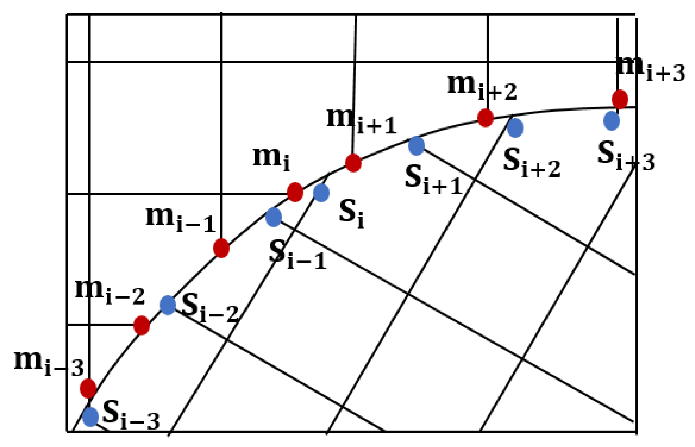
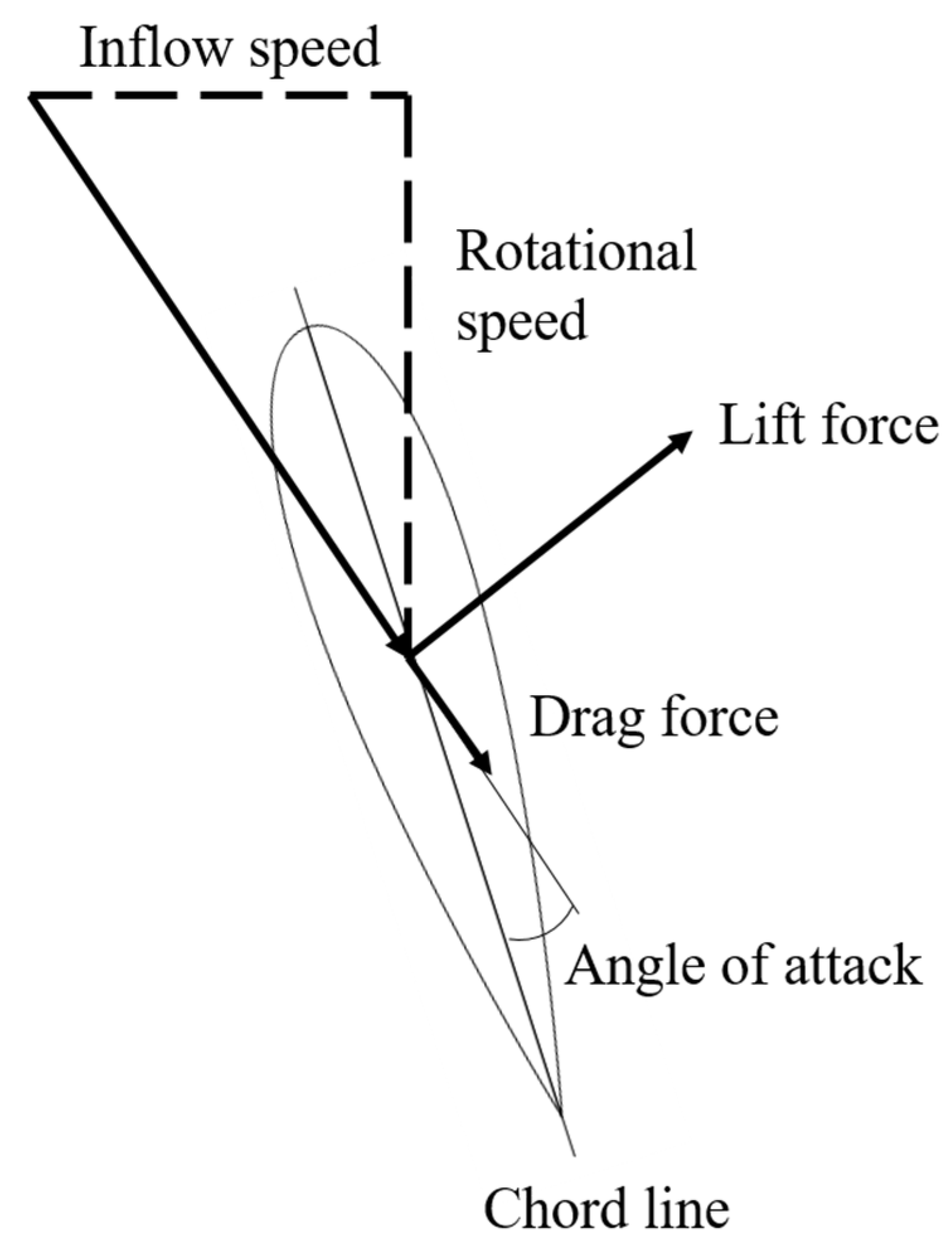
2.1. Governing Equations

The governing equations for the computational simulation are the continuity and RANS equations for incompressible flow,
u i ¯ x i = 0 ,
u i ¯ t + ( u i ¯ u j ¯ ) x j = 1 ρ p ¯ x j + x j ( u i ¯ x j τ i j ) ,  
where u i ¯ and p ¯ are the time-averaged velocity and pressure, respectively. The Reynolds stress tensor, τ i j , incorporates the effect of turbulent motions in the mean stresses. The closure for the Reynolds stress terms is treated by the k - ω shear stress transport (SST) model using the Bouissinesq approximation. The k SST model [18,19] is suitable for flows with strong adverse pressure gradient and reverse flow. For this reason, it is often used to simulate the flow around turbines and propellers. The k-ω SST model is a combination of the original Wilcox k-ω model [20] and the standard k-ϵ model. The k-ω SST model is for near walls and k-ϵ model is for regions away from walls. The eddy viscosity formula is used for the transport of principle turbulent shear stress:
τ i j = 2 ν S i j ¯ + 2 3 k δ i j
where ν represents the eddy viscosity, obtained from
ν = k ω .
In Equation (4) k is the turbulence kinetic energy, and ω is the rate of dissipation of the eddies. S i j ¯ is the symmetric tensor of mean strain rate:
S i j ¯ = 1 2 ( u i ¯ x j + u j ¯ x i ) .  
The equations for the k - ω SST model are
k t + u j k x j = P β * k ω + x j ( ( ν + ν t σ k ) k x j ) ,  
ω t + u j ω x j = α ω k P β ω 2 + x j ( ( ν + ν σ ω ) ω x j ) + 2 ( 1 F 1 ) σ ω 2 1 ω k x j ω x j .
The model constants are
P = τ i j u i x j   ,         ν = k ω       ,     F 1 = tan h ( k β * ω d ) ,
where β * = 0.09 , α = 5 / 9 , β = 0.075 , σ k = 2.0 and σ ω = 2.0 .
The time discretization method was the Crank–Nicolson method with second-order accuracy. Velocity and turbulence properties were discretized by a second-order upwind scheme. The pressure velocity coupling was implemented using the PIMPLE algorithm [21], which is a combination of Pressure Implicit with Splitting of Operator (PISO) and Semi-Implicit Method for Pressure-Linked Equations (SIMPLE) algorithms.

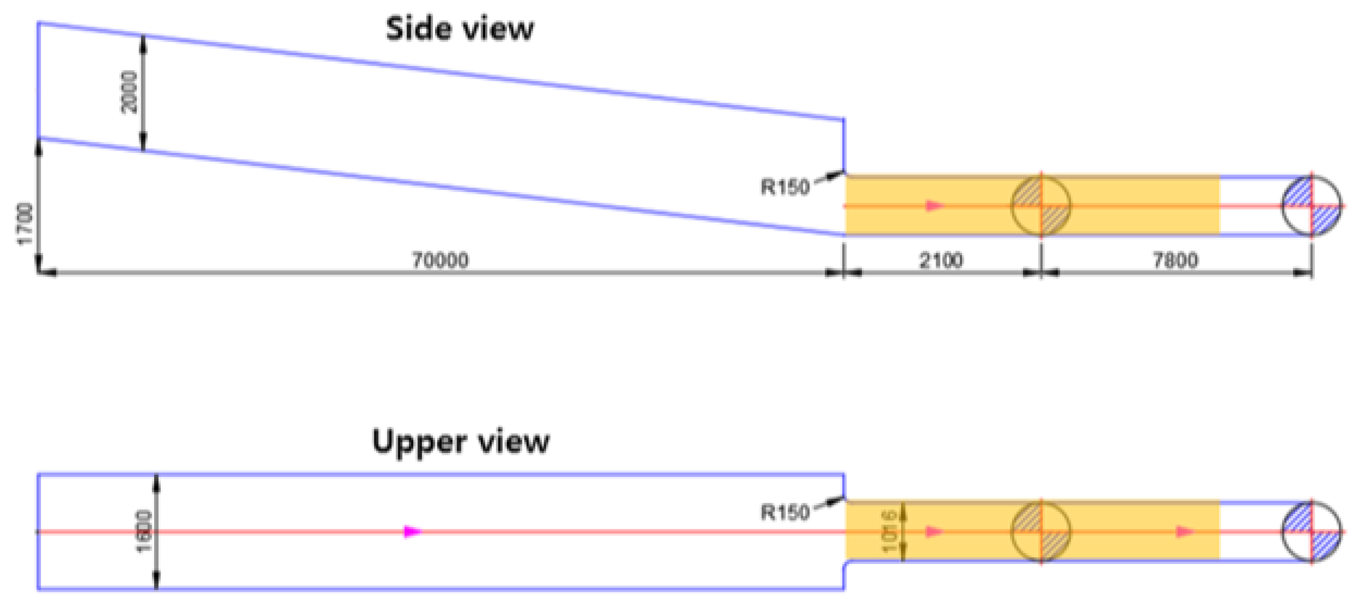
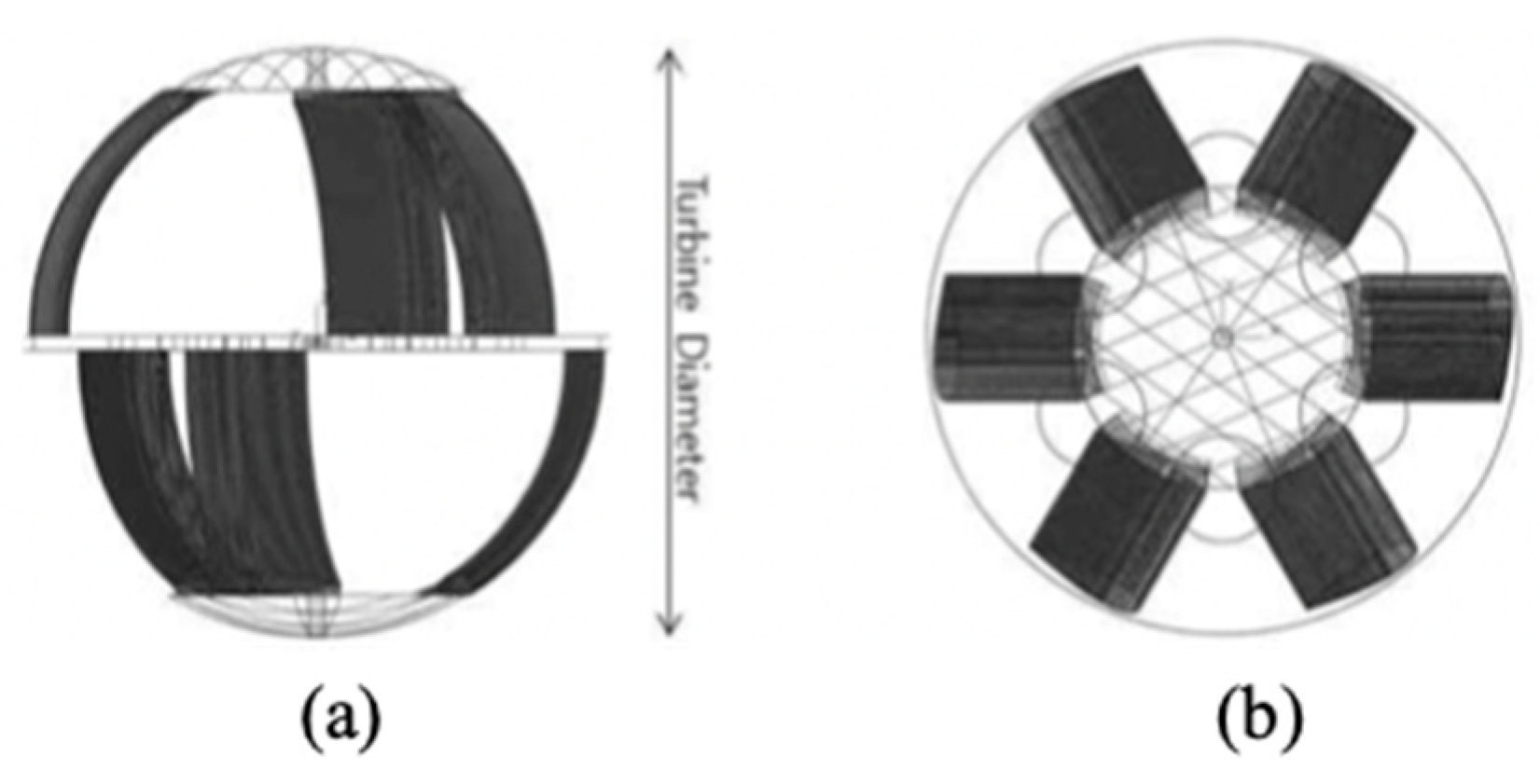
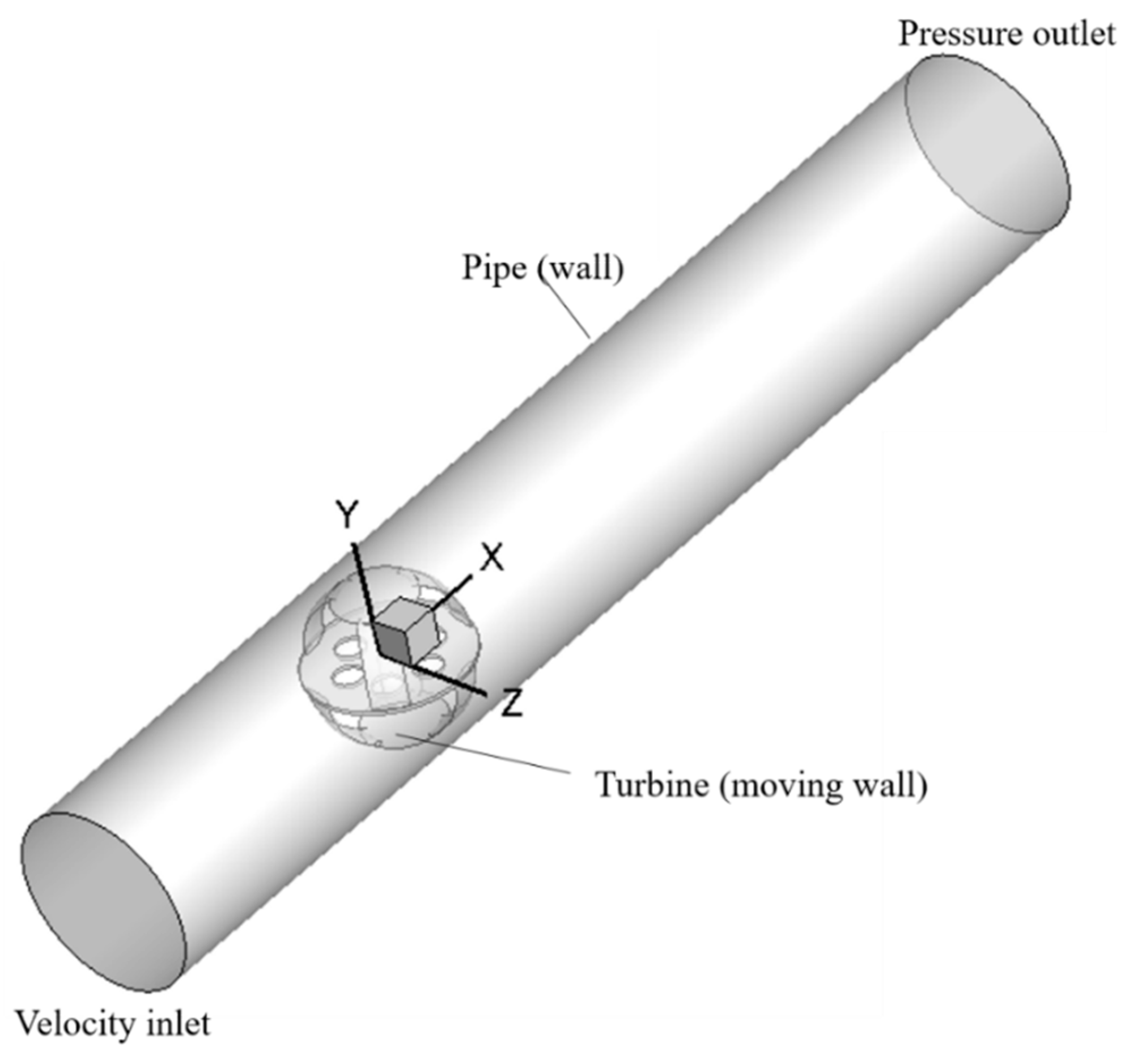
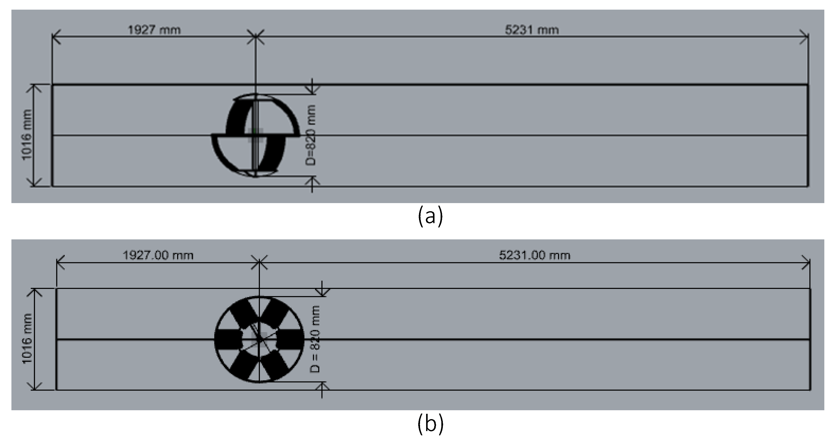
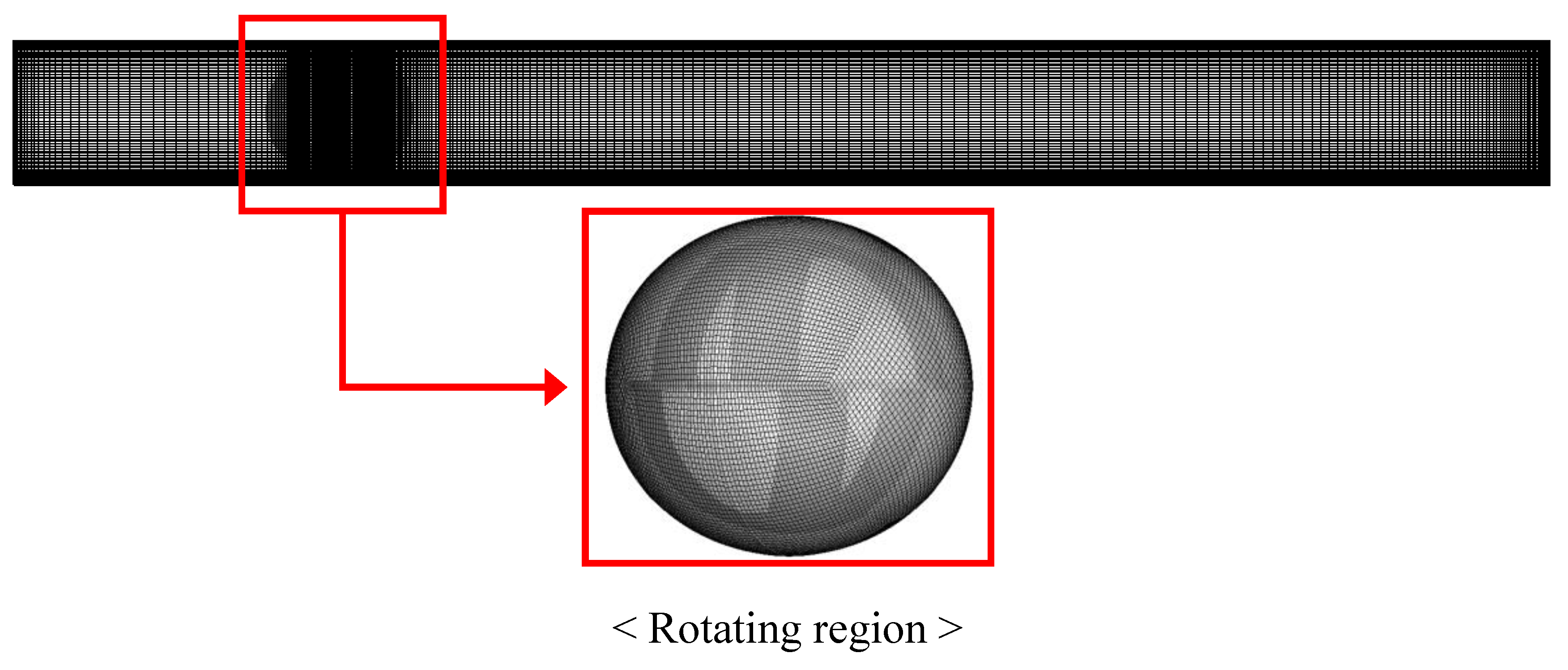
2.2. Computational Domain, Mesh and Boundary Conditions

The turbine designed for the present study was installed in a water pipe for a drain system. A simplified drain system model is shown in Figure 1. Water in the drain system flowed due to gravity with a head of 1700 mm and entered the water pipe with the diameter of 1016 mm. The size of the turbine was selected based on a turbine design of the highest energy-collection efficiency at a fixed flow rate, water pipe size, installation effectiveness, maintenance and foreign substances in the given operating conditions. As shown in Figure 2, the shape of the turbine was spherical with a diameter of 820 mm and composed of six vertical blades of the NACA 0020 cross section. Figure 3 shows the coordinate system and boundary conditions. The origin is at the center of the turbine, the x-direction is parallel to the flow direction and the y-direction is along the turbine rotation axis. Figure 4 shows the turbine in the computational domain. The turbine was located 2.35   D t u r b i n e downstream from the inlet, and 6.38   D t u r b i n e upstream from the outlet. In order to represent the rotating motion of the turbine, two sub-domains were generated. As shown in Figure 5, the one was the spherical inner sub-domain that contained the turbine, and the other was the outer sub-domain surrounding the inner spherical domain. For the boundary conditions, the Dirichlet velocity condition was applied to the inlet with a constant flow speed (7.3 m/s). The no-slip boundary condition was applied to the water pipe and the turbine surface.
An interpolation was used for the arbitrary mesh interface (AMI) boundary condition at the interface between the two sub-domains. The interpolation was done by the formula in Equation (9), which is illustrated in Figure 6. In Equation (9), s i is the estimated physical quantity of the i-th node of a domain and m j is the quantity of the j-th node of the other sub-domain. d i , j denotes the distance between two nodes. The efficiency was calculated and compared based on TSR, which was calculated by Equation (10).
s i = ( d i , j 1 + d i , j + 1 ) m j 2 ( d i , j + d i , j 1 + d i , j + 1 ) + ( d i , j + d i , j + 1 ) m j 1 2 ( d i , j + d i , j 1 + d i , j + 1 ) + ( d i , j + d i , j 1 ) m j + 1 2 ( d i , j + d i , j 1 + d i , j + 1 ) .
λ = R Ω V i n l e t .
To investigate the tip clearance effects, turbine performance was compared for different turbine sizes with a fixed pipe diameter. The tip clearance (t) was defined as in Equation (11), and three different turbine sizes corresponded to tip clearances of 19.3%, 15.0% and 12.0%, respectively. Tip clearances were determined from the turbine size, which was suggested by the manufacturer. Figure 7 shows the detailed view of the different meshes with the different tip clearances.
t = D p i p e D t u r b i n e D p i p e × 100   ( % ) .

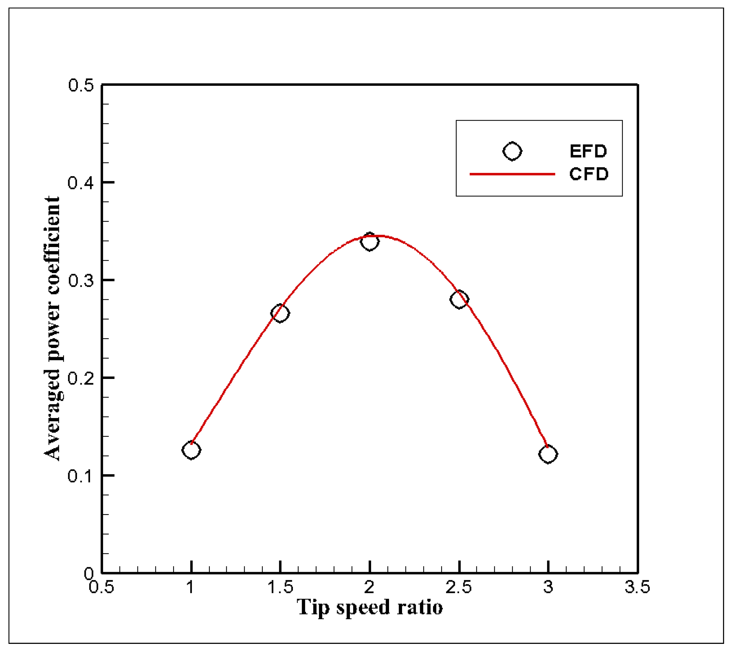
2.3. CFD Solver Validation

The CFD solver was validated for the Darrieus turbine. A simple shape of a fixed-pitch vertical-axis water turbine [22] was used for the validation. Figure 8 illustrates the test configuration and computational domain. The diameter of the Darrieus turbine (D) was 175 mm, and its height (H) was 175 mm. The blade’s cross section shape was a modified NACA 0018 section, and the chord length was 32 mm. The turbine’s rotation axis was located 525 mm (3D) downstream from the inlet and 1225 mm (7D) upstream from the outlet. The same boundary conditions described in the previous section were applied.
The Reynolds number was based on the blade chord length (C), as
R e C = ρ C Ω R μ = λ ρ C V i n l e t μ ,
where ρ is density of water, Ω is the turbine rotation speed, μ is the dynamic viscosity of water and λ is TSR. The turbine performance was analyzed with a constant inlet speed (2.3 m/s) and various TSRs of 1.0, 1.5, 2.0, 2.5 and 3.0, which were adopted from the experimental conditions [22].
The experimental and computational results for the instantaneous power coefficients are shown in Figure 9. The power coefficients show good agreement within the 5% level. Figure 10 presents the averaged experimental and computational power coefficients. The CFD results were estimated to be 2% to 3% higher than the experimental results, but within the experimental error range of 6% to 10% [22].

3. Results and Discussion

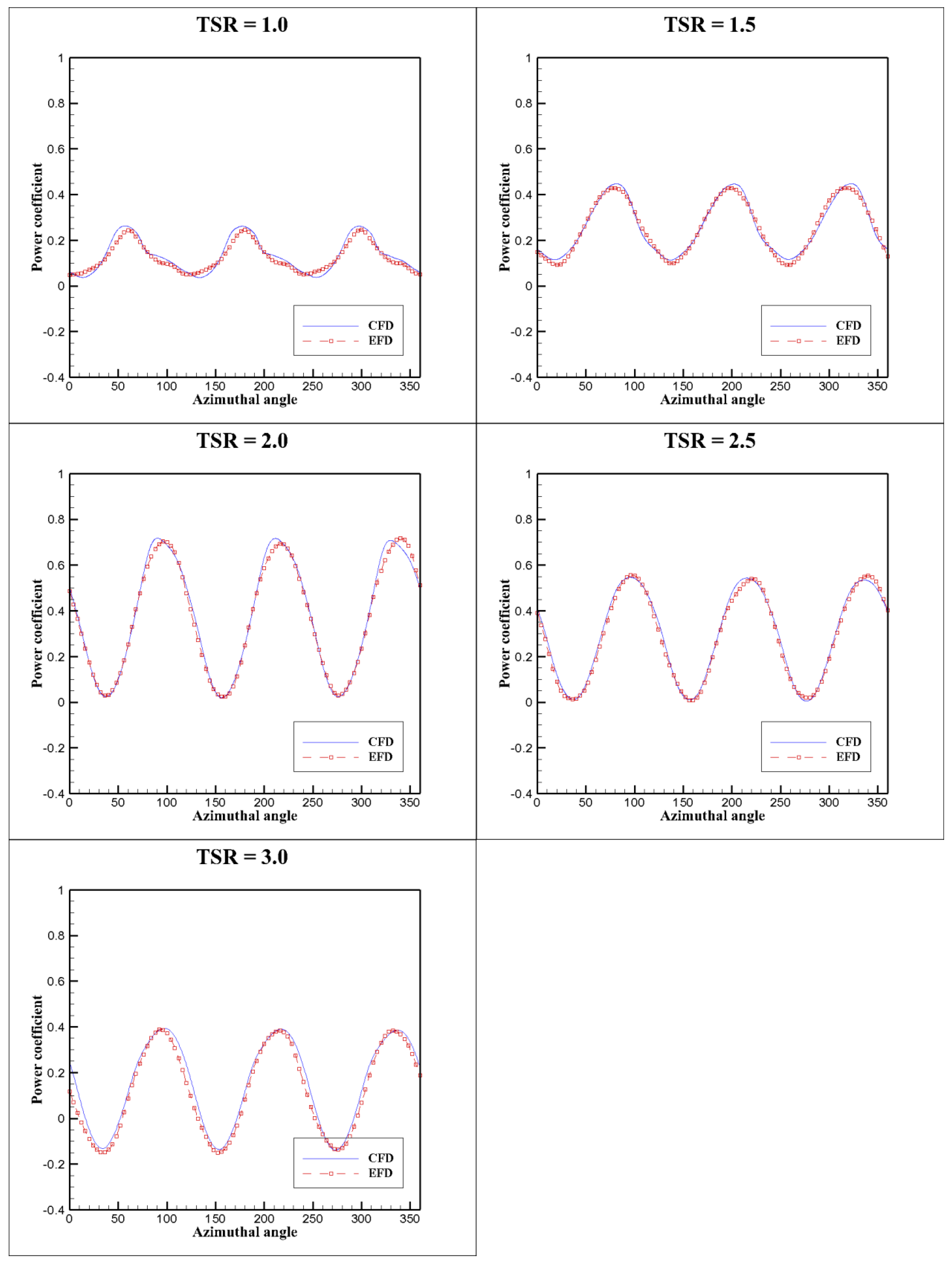
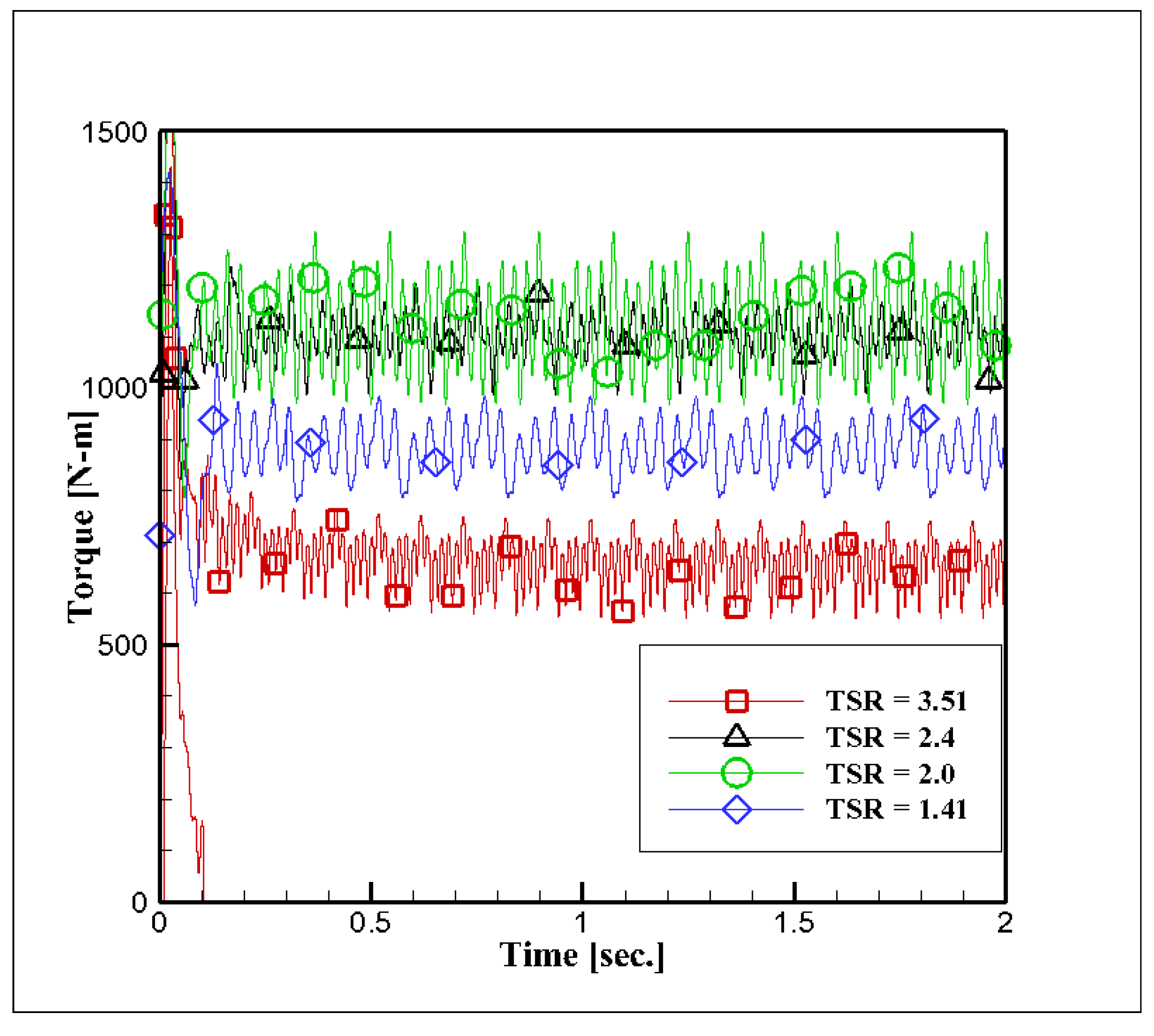
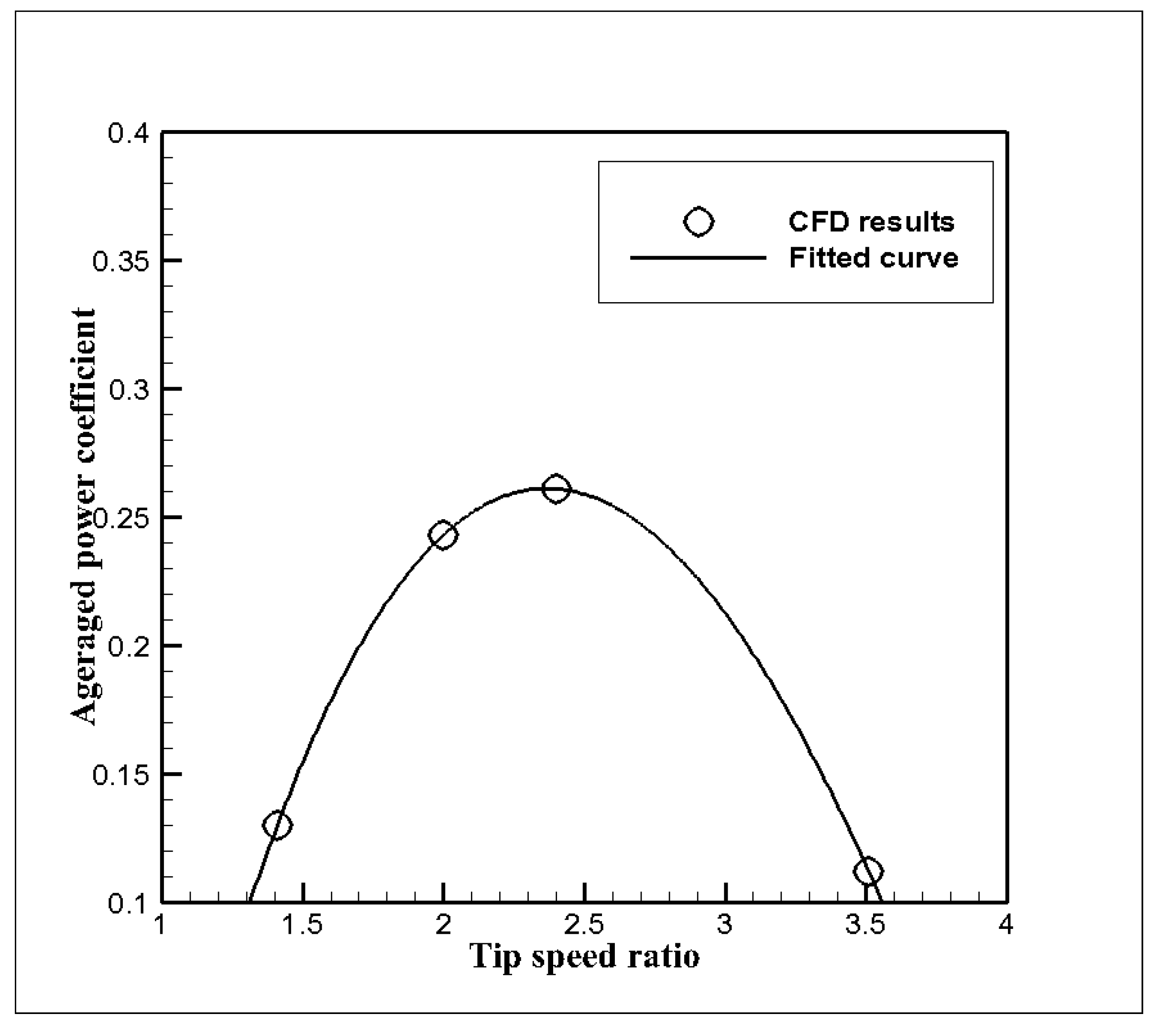
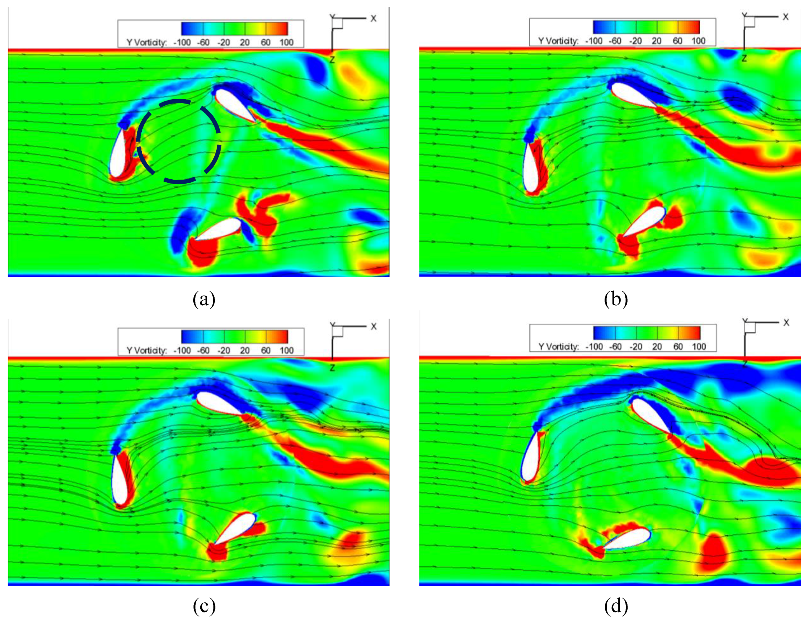
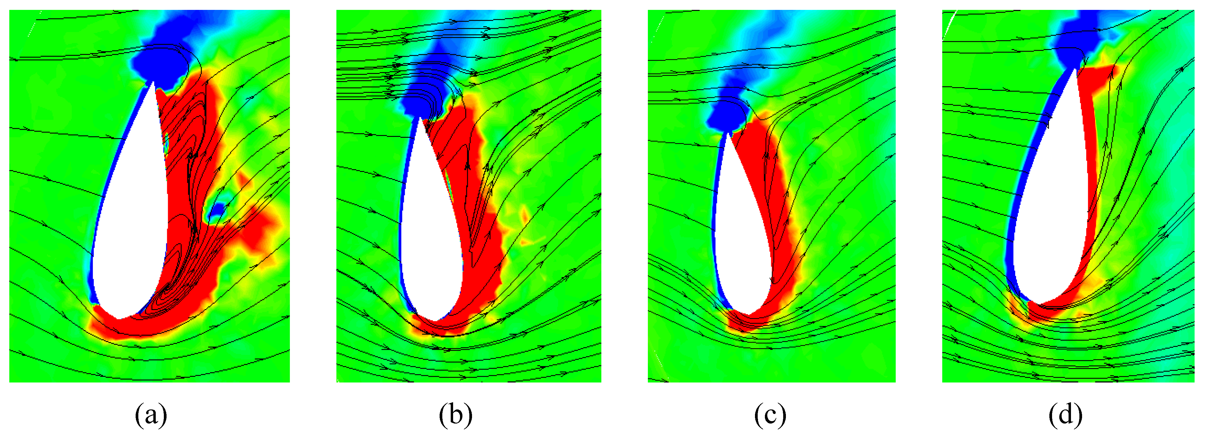
3.1. Performance Analysis with Respect to TSR

To determine the optimal operating conditions of the turbine, we conducted performance analyses at four different TSRs. In case of Maître [22], the highest efficiency was identified at TSR = 2.0. So, the analysis was performed around TSR = 2.0 (TSR = 1.41, TSR = 2.0 and TSR = 2.4) and a higher condition (TSR = 3.51). Figure 11 shows time history of torque acting on the turbine. As shown in Figure 11, the turbine produced the highest torque at a TSR of 2.4 and the lowest one at a TSR of 3.51. The power (Pturbine) collected by the turbine can be calculated using Equation (13):
P t u r b i n e = T t u r b i n e × Ω
where T t u r b i n e is torque of the turbine and Ω is an angular velocity. The power was normalized introducing the power coefficient ( C P ) as follows:
C P = P t u r b i n e 1 2 ρ A V i n l e t 3 = T t u r b i n e Ω 1 2 ρ A V i n l e t 3 ,
where A is the cross-sectional area of the turbine.
The denominator in Equation (14) represents the total energy of the inlet flow into the pipe. We used the same pipe diameter and inflow velocity, thus the power coefficient was influenced by TSR only. According to Seo et al. [9], the variation of turbine performance in different TSR conditions was directly affected by changes in the angle of attack onto the blade section. Figure 12 shows an angle of attack and the forces on the turbine blade section. If the TSR is reduced, the rotation speed of the turbine slowed down, and then the angle of attack increased. The high angle of attack induced the higher lift and moment generated by the turbine.
In the present case, as shown in Figure 13, TSR = 2.4 was the optimal condition. In the low TSR cases, the torque generated by the turbine was less than the torque in optimal condition due to the stall on the blade surfaces. Figure 14 shows Y-vorticity and streamlines on a y = 0.1 D t u r b i n e plane and Figure 15 shows the zoom-in views on Blade 1. In Figure 14a and Figure 15a, separation was observed near the leading edge. However, at other TSRs, separation was observed at the mid chord (TSR = 2.0) and trailing edge (TSR = 2.4 and TSR = 3.51). Downstream flow around the blades was less disturbed at a high TSR than a low TSR. Separation from the blade surfaces disturbed downstream flow. The heavily disturbed flows resulted in less power generation.

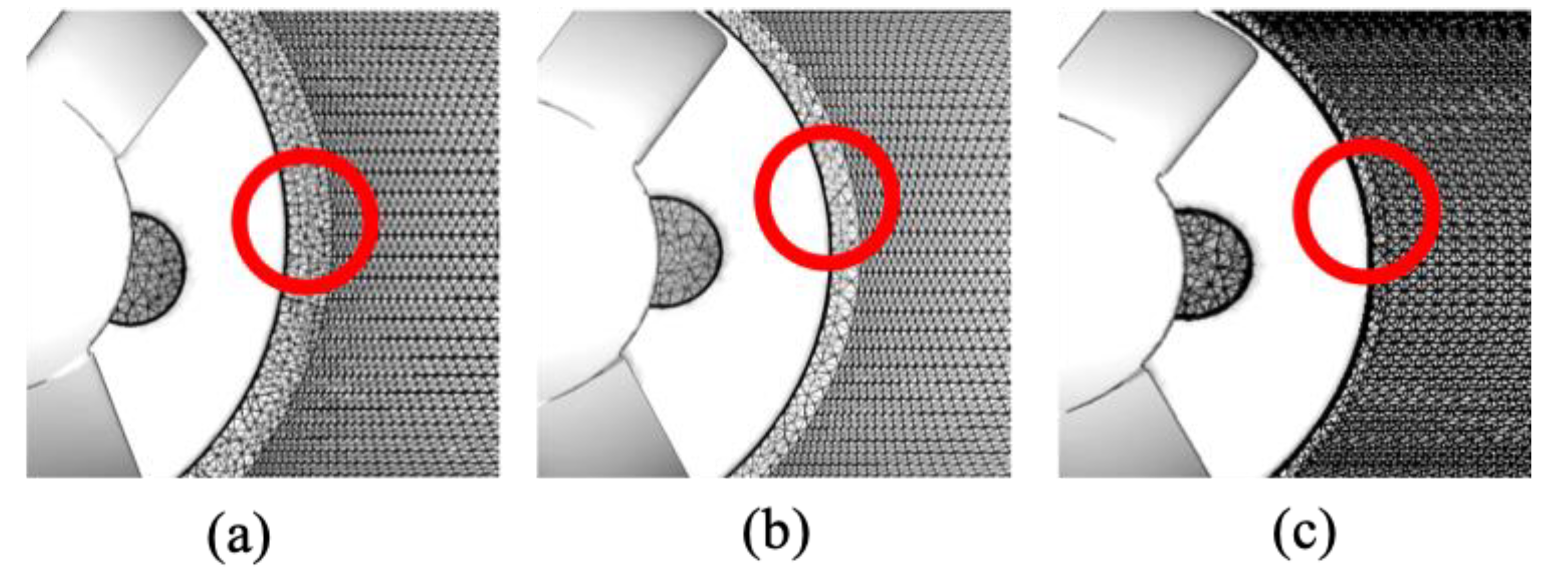
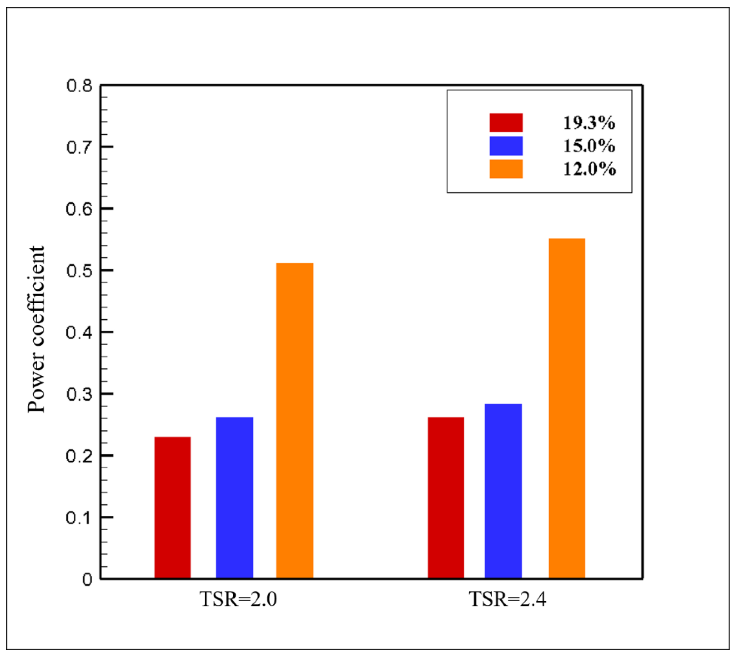
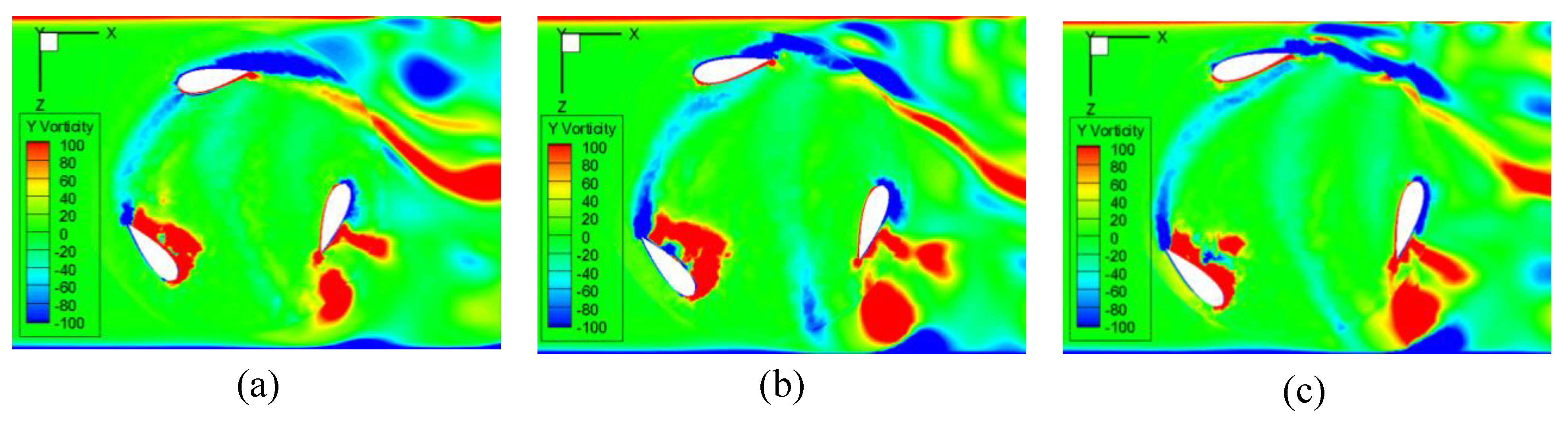
3.2. Performance Analysis with Respect to Tip Clearance

The turbine’s best performance was achieved at a TSR of 2.4, as described in the previous section. The effects of the tip clearance on the turbine performance was analyzed at two TSRs, 2 and 2.4, by considering three different size turbines. Figure 16 shows the power coefficient with respect to the tip clearance. The power coefficient dramatically increased as tip clearance was reduced. The power coefficient of the tip clearance of 15.0% case was about 3% higher than that of the 19.3% case, and the power coefficient of the tip clearance of 12.0% case was about 25% higher than that of the 15.0% case.
Figure 17 shows the Y-vorticity contours on the y = 0.1 D t u r b i n e plane and Figure 18 shows streamlines emanating from the plane at y = 0.1 D t u r b i n e . The smaller tip clearance was, the smaller the vortical structure was separated from the trailing edge. It means that the downstream flow was less disturbed in the small tip clearance case, and thus more power was generated. The wake behind the forward blade also affected the following blade.
In the tip clearance of 19.3% case, the wake behind the forward blade affected the inflow of following blade directly as shown in Figure 17a. In the smaller tip clearance case, the inflow of the following blade had less influence. The clear inflow led to more power generation. In Figure 18, the streamlines of the flow disturbed by the turbine are shown downstream. With a tip clearance of 19.3%, this three-dimensional flow development was the most conspicuous with a ribbon-shaped wake flow. However, as the tip clearance decreases, the streamlines were less complicated. It was evident that the smaller tip clearance resulted in less energy wasted in forming the wake flow, which would be correlated to a higher energy-collection efficiency.

4. Summary and Conclusion

In this study, the optimized operating conditions were identified for the vertical-axis turbine for collecting the unused water energy in a water pipe and the effects of the tip clearance between the turbine and the pipe wall on the turbine performance were examined. The target turbine was a spherical turbine consisting of six crossed wings selected through model tests and the cross section of each wing was made of NACA 0020.
The turbine showed the highest efficiency and power at TSR = 2.4, and it was identified that the turbine can collect about 26.1% energy from the flow in the pipe. At a small TSR, the angle of attack increased and the torque acting on the turbine also increased. If the angle of attack was too large, the torque was reduced by the stall. It illustrated a trade-off between torque generation and turbine rotating speed. The separation from the blade at the upstream also disturbed the downstream flow. The effect of tip clearance was analyzed at TSRs of 2 and 2.4. The results showed that the turbine with a small tip clearance showed a high efficiency in energy-collection. The Y-vorticity contours and wake streamline were examined to analyze the local flow features around the turbine. The turbine with a small tip clearance accompanied small vortical structures separated from the trailing edge. Furthermore, greater tip clearance made the wake flow more complicated. But the wake flow became smoother as the tip clearance decreased. It showed that a smaller tip clearance resulted in less energy wasted in the wake.

Author Contributions

Writing-original draft, H.Y. and W.S.; Investigation & software, S.S.; Turbine design, C.-S.M.; Conceptualization, B.C.J. and Y.C.H.; Supervision, W.S. and S.H.R.; Project administration, S.H.R.

Acknowledgments

This research was supported by the Korea Institute of Energy Technology Evaluation and Planning (KETEP), granted financial resource from the Ministry of Trade, Industry & Energy, Republic of Korea (No. 20162010104420), the National Research Foundation of Korea (NRF-2017K1A3A1A19071629) and Institute of Engineering Research at Seoul National University.

Conflicts of Interest

The authors declare no conflict of interest.

Nomenclature

D t u r b i n e Turbine diameter (m)
D p i p e Pipe diameter (m)
Ω Turbine rotation speed (rad/s)
V i n l e t Inlet flow velocity (m/s)
λ Tip speed ratio (-)
t Tip clearance (m)
T t u r b i n e Torque produced by turbine (N·m)
P t u r b i n e Power output (W)
C P Power coefficient (-)
C p r e s s Pressure coefficient (-)

References

  1. Kyono, T.; Suzuki, R.O.; Ono, K. Conversion of unused heat energy to electricity by means of thermoelectric generation in condenser. IEEE Trans. Energy Convers. 2003, 18, 330–334. [Google Scholar] [CrossRef]
  2. Datta, R.; Ranganathan, V.T. A method of tracking the peak power points for a variable speed wind energy conversion system. IEEE Trans. Energy Convers. 2003, 18, 163–168. [Google Scholar] [CrossRef]
  3. Muetze, A.; Vining, J.G. Ocean wave energy conversion—A survey. In Proceedings of the Conference Record of the 2006 IEEE Industry Applications Conference Forty-First IAS Annual Meeting, Tampa, FL, USA, 8–12 October 2006; Volume 3, pp. 1410–1417. [Google Scholar]
  4. Moheimani, N.R.; Parlevliet, D. Sustainable solar energy conversion to chemical and electrical energy. Renew. Sustain. Energy Rev. 2013, 27, 494–504. [Google Scholar] [CrossRef]
  5. Okajima, I.; Sako, T. Energy conversion of biomass with supercritical and subcritical water using large-scale plants. J. Biosci. Bioeng. 2014, 117, 1–9. [Google Scholar] [CrossRef] [PubMed]
  6. Khan, M.J.; Bhuyan, G.; Iqbal, M.T.; Quaicoe, J.E. Hydrokinetic energy conversion systems and assessment of horizontal and vertical axis turbines for river ad tidal applications: A technology status review. Appl. Energy 2009, 86, 1823–1835. [Google Scholar] [CrossRef]
  7. Bahaj, A.S.; Molland, A.F.; Chaplin, J.R.; Batten, W.M.J. Power and thrust measurements of marine current turbines under various hydrodynamic flow conditions in a cavitation tunnel and a towing tank. Renew. Energy 2007, 32, 407–426. [Google Scholar] [CrossRef]
  8. Lee, J.H.; Park, S.; Kim, D.H.; Rhee, S.H.; Kim, M.C. Computational methods for performance analysis of horizontal axis tidal stream turbines. Appl. Energy 2012, 98, 512–523. [Google Scholar] [CrossRef]
  9. Seo, J.; Lee, S.J.; Choi, W.S.; Park, S.T.; Rhee, S.H. Experimental study on kinetic energy conversion of horizontal axis tidal stream turbine. Renew. Energy 2016, 97, 784–797. [Google Scholar] [CrossRef]
  10. Tedds, S.C.; Owen, I.; Poole, R.J. Near-wake characteristics of a model horizontal axis tidal stream turbine. Renew. Energy 2014, 63, 222–235. [Google Scholar] [CrossRef] [Green Version]
  11. Myers, L.; Bahaj, A.S. Wake studies of a 1/30th scale horizontal axis marine current turbine. Ocean Eng. 2007, 34, 758–762. [Google Scholar] [CrossRef]
  12. Yang, P.; Xiang, J.; Fang, F.; Pain, C.C. A fidelity fluid-structure interaction model for vertical axis tidal turbines in turbulence flows. Appl. Energy 2019, 236, 465–477. [Google Scholar] [CrossRef]
  13. Ouro, P.; Runge, S.; Luo, Q.; Stoesser, T. Three-dimensionality of the wake recovery behind a vertical axis turbine. Renew. Energy 2019, 133, 1066–1077. [Google Scholar] [CrossRef]
  14. Jung, H.J.; Lee, J.H.; Rhee, S.H.; Song, M.; Hyun, B.S. Unsteady flow around a two-dimensional section of a vertical axis turbine for tidal stream energy conversion. Int. J. Nav. Archit. Ocean Eng. 2009, 1, 64–69. [Google Scholar] [CrossRef] [Green Version]
  15. Han, J.S.; Choi, D.H.; Hyun, B.S.; Kim, M.C.; Rhee, S.H.; Song, M.S. Parametric Numerical Study on the Performance of Helical Tidal Stream Turbines. J. Korean Soc. Mar. Environ. Energy 2011, 14, 114–120. [Google Scholar] [CrossRef]
  16. Chen, J.; Yang, H.X.; Liu, C.P.; Lau, C.H.; Lo, M. A novel vertical axis water turbine for power generation from water pipelines. Energy 2013, 54, 184–193. [Google Scholar] [CrossRef]
  17. Lucid Energy/LucidPipeTM Power System. February 2016. Available online: http://www.lucidenergy.com/how-it-works/ (accessed on 21 July 2019).
  18. Menter, F.R. Influence of freestream values on k-omega turbulence model prediction. AIAA J. 1992, 30, 1657–1659. [Google Scholar] [CrossRef]
  19. Menter, F.R. Two-equation eddy-viscosity turbulence models for engineering applications. AIAA J. 1994, 32, 1598–1605. [Google Scholar] [CrossRef] [Green Version]
  20. Wilcox, D.C. Formulation of the turbulence model revisited. AIAA J. 2008, 46, 2823–2838. [Google Scholar] [CrossRef]
  21. Chen, L.F.; Zang, J.; Hillis, A.J.; Morgan, G.C.J.; Plummer, A.R. Numerical investigation of wave–structure interaction using OpenFOAM. Ocean Eng. 2014, 88, 91–109. [Google Scholar] [CrossRef]
  22. Maître, T.; Amet, E.; Pellone, C. Modeling of the flow in a Darrieus water turbine: Wall grid refinement analysis and comparison with experiments. Renew. Energy 2013, 51, 497–512. [Google Scholar] [CrossRef]
Figure 1. A schematic view of the drain system.
Energies 12 03998 g001
Figure 2. Turbine design: (a) side view and (b) top view.
Energies 12 03998 g002
Figure 3. Coordinate system and boundary conditions.
Energies 12 03998 g003
Figure 4. Vertical axis turbine installed in a water pipe: (a) side view and (b) top view.
Energies 12 03998 g004
Figure 5. Computational domains and mesh.
Energies 12 03998 g005
Figure 6. Physics quantity interpolation between the arbitrary mesh interface.
Energies 12 03998 g006
Figure 7. Detailed view of the tip clearance and domain interface: (a) 19.3% clearance, (b) 15.0% clearance and (c) 12.0% clearance.
Energies 12 03998 g007
Figure 8. Computational domain for the Darrieus turbine: (a) side view and (b) top view.
Energies 12 03998 g008
Figure 9. Time histories of CP of the Darrieus turbine at various tip-speed ratios (TSRs).
Energies 12 03998 g009
Figure 10. Averaged power coefficients of the Darrieus turbine at various TSRs.
Energies 12 03998 g010
Figure 11. Time history of torque on the turbine.
Energies 12 03998 g011
Figure 12. Schematic diagram of the angle of attack and force acting on the cross section of the turbine blade.
Energies 12 03998 g012
Figure 13. Averaged power coefficient of the spherical turbine with respect to TSR.
Energies 12 03998 g013
Figure 14. Y-vorticity contours and streamlines on y = 0.1D_turbine at (a) TSR = 1.41, (b) TSR = 2.00, (c) = TSR = 2.40 and (d) TSR = 3.51.
Energies 12 03998 g014
Figure 15. Zoom on Blade 1 at (a) TSR = 1.41, (b) TSR = 2.00, (c) = TSR = 2.40 and (d) TSR = 3.51.
Energies 12 03998 g015
Figure 16. Power coefficient of the turbine with respect to tip clearance.
Energies 12 03998 g016
Figure 17. Y-vorticity contours on y = 0.1D_turbine at TSR = 2.4 with a tip clearance of (a) 19.3%, (b) 15.0% and (c) 12.0%.
Energies 12 03998 g017
Figure 18. Wake flow streamlines configuration with tip clearance: (a) 19.3%, (b) 15.0% and (c) 12.0%, respectively.
Energies 12 03998 g018

