Review

Review and Comparison of Intelligent Optimization Modelling Techniques for Energy Forecasting and Condition-Based Maintenance in PV Plants

by
Jesús Ferrero Bermejo
1,
Juan Francisco Gómez Fernández
2,
Rafael Pino
3,
Adolfo Crespo Márquez
2,* and
Antonio Jesús Guillén López
2
1
Magtel Operaciones, 41940 Seville, Spain
2
Department of Industrial Management, Escuela Técnica Superior de Ingenieros, 41092 Sevilla, Spain
3
Department of Statistics and Operations Research, Facultad de Matemáticas, Universidad de Sevilla, 41012 Sevilla, Spain
*
Author to whom correspondence should be addressed.
Submission received: 19 September 2019 / Revised: 15 October 2019 / Accepted: 29 October 2019 / Published: 31 October 2019
(This article belongs to the Special Issue Intelligent Optimization Modelling in Energy Forecasting)

Abstract

:
Within the field of soft computing, intelligent optimization modelling techniques include various major techniques in artificial intelligence. These techniques pretend to generate new business knowledge transforming sets of "raw data" into business value. One of the principal applications of these techniques is related to the design of predictive analytics for the improvement of advanced CBM (condition-based maintenance) strategies and energy production forecasting. These advanced techniques can be used to transform control system data, operational data and maintenance event data to failure diagnostic and prognostic knowledge and, ultimately, to derive expected energy generation. One of the systems where these techniques can be applied with massive potential impact are the legacy monitoring systems existing in solar PV energy generation plants. These systems produce a great amount of data over time, while at the same time they demand an important effort in order to increase their performance through the use of more accurate predictive analytics to reduce production losses having a direct impact on ROI. How to choose the most suitable techniques to apply is one of the problems to address. This paper presents a review and a comparative analysis of six intelligent optimization modelling techniques, which have been applied on a PV plant case study, using the energy production forecast as the decision variable. The methodology proposed not only pretends to elicit the most accurate solution but also validates the results, in comparison with the different outputs for the different techniques.

Graphical Abstract

1. Introduction

Within the field of soft computing, intelligent optimization modelling techniques include various major techniques in artificial intelligence [1] pretending to generate new business data knowledge transforming sets of "raw data" into business value. In the Merriam-Webster dictionary data mining is defined as “the practice of searching through large amounts of computerized data to find useful patterns or trends”, so we can then say that intelligent optimization modelling techniques are data mining techniques.
Nowadays, connections among industrial assets and integrating information systems, processes and operative technicians [2] are the core of the next-generation of industrial management. Based on the industrial Internet of Things (IoT), companies have to seek intelligent optimization modelling techniques (advanced analytics) [3] in order to optimize decision-making, business and social value. These techniques are preferred to fall inside the soft computing category, with the idea of solving real complex problems with inductive reasoning like humans, searching for probable patterns, being less precise, but adaptable to reasonable changes and easily applicable and obtainable [4].
To be able to implement these advanced techniques requires a comprehensive process sometimes named “intelligent data analysis” (IDA) [5], which is a more extensive and non-trivial process to identify understandable patterns from data. Within this process, the main difficulty is to identify valid and correct data for the analysis [3] from the different sources in the company. Second, efforts must be developed to create analytic models that provide value by improving performance. Third, a cultural change has to be embraced for companies to facilitate the implementation of the analytical results. In addition to this, since accumulation of data is too large and complex to be processed by traditional database management tools (the definition of “big data” in the Merriam-Webster dictionary), new tools to manage big data must be taking into consideration [6].
Under these considerations IDA can be applied to renewable energy production, as one of the most promising fields of application of these techniques [7]. The stochastic nature of these energy sources, and the lack of a consolidated technical background in most of these technologies, make this sector very susceptible for the application of intelligent optimization modelling techniques. The referred stochastic nature is determined by circumstances in the generation sources, but also by the existing operational conditions. That is, the natural resources have variations according to weather with a certain stationarity but with difficulties in forecasting behaviours. In addition, depending on the operational and environmental stresses in the activities, they will be more likely to fail. Consequently, the analysis of renewable energy production must consider adaptability to dynamic changes that can yield results [8].
The identification and prediction of potential failures can be improved using advanced analytics as a way to search proactively and reduce risk in order to improve efficiency in energy generation. Algorithms, such as machine learning, are now quite extended in renewable energy control systems. These kinds of facilities are characterized by the presence of a great number of sensors feeding the SCADA systems (supervisory control and data acquisition systems), usually very sophisticated systems including a control interface and a client interface (the plant’s owner, distribution electric network administrator, etc.). Power and energy production measures are two of the most important variables managed by the SCADA. As principal system performance outputs, they can be exploited through data mining techniques to control system failures, since most of the systems failures directly affect the output power and the energy production efficiency [7].
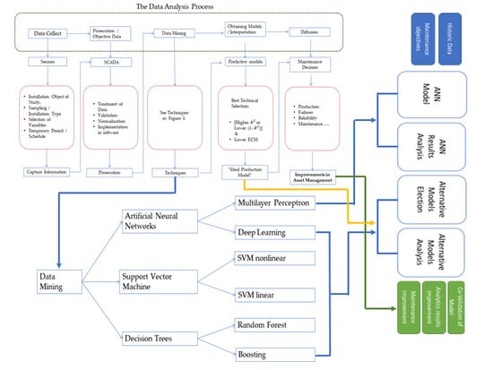
A sample process for a comprehensive IDA, applied to the improvement of assets management in renewable energy, is presented in Figure 1.
In Figure 1 the green box describes the generic IDA process phases, phases which need to be managed inside an asset management condition-based maintenance (CBM) framework, in order to make sustainable and well-structured decisions, to obtain developments and to keep and improve solutions over time. In order to take rapid and optimal decisions, the challenge is to structure the information from different sources, synchronizing it properly in time, in a sustainable and easily assimilable way, reducing the errors (avoiding dependencies among variables, noise, and interferences) and valuing real risks. A clear conceptual framework allows the permanent development of current and new algorithms, corresponding to distinct data behaviour-anomalies with physical degradation patterns of assets according to their operation and operation environment conditions and their effects on the whole plant [11].
Each one of these IDA phases are interpreted, in the red boxes, for a PV energy production data system [9,10] showing a flow-chart for practical implementation. In this paper we will focus on the central phase in Figure 1, the analysis of different techniques of data mining (DM). Different techniques can be applied. We will concentrate in the selection of advanced DM techniques, comparing their results when applied to a similar case study. This issue is often not addressed when applying certain complex intelligent optimization modelling techniques, and no discussion emerges concerning this issue. This is because, often, the computational effort to apply a certain method is very important in order to be able to benchmark the results of several methods [12]. In the future, assuming more mature IDA application scenarios, the selection of DM techniques will likely be crucial to generating well-informed decisions.
Accepting this challenge, a review of the literature, the selection of techniques and a benchmark of their results are presented in this paper. According to the previous literature, most representative techniques of data mining [13,14] are presented and applied to a case study in a photovoltaic plant (see other examples where these techniques were applied in Table 1).
Artificial neural networks (ANN) have been largely developed in recent years. Some authors [15,16,17,18,19,20] have focused on obtaining PV production predictions through a behavioural pattern that is modelled by selected predictor variables. A very interesting topic is how these results can be applied in predictive maintenance solutions. In [7] these models are used to predict PV system’s faults before they occur, improving the efficiency of PV installations, allowing programming in advance of suitable maintenance tasks. Following a similar approach, the rest of DM techniques are implemented to validate, or even improve, the good results obtained with the ANN in terms of asset maintenance and management.
In general terms, the results obtained using DM or machine learning to follow and predict PV critical variables, like solar radiation [21], are good enough to use as inputs in decision-making processes, like maintenance decisions [7]. However, not all of the techniques have the same maturity level as ANNs. SVM, Random Forest and Boosting, as techniques to predict the yield of a PV plant, should be studied in greater depth in the coming years [22].

2. Background

2.1. Data Mining Techniques

Data mining techniques are in constant development by combining the use of the diverse techniques available over a wide range of application fields. The search of behavioural patterns or predictions based on various predictive variables that allow us to know the future or expected outcome to improve key decision-making is being extended by researching the most diverse application fields. For example, in [23] the assessment of credit ratings from a risk perspective, using different data mining techniques and hybrid models, are proposed, analysing the advantages and disadvantages of each. In a completely different application field, [24,25] present models of distribution of solar spectral radiation based on data mining techniques, using solar irradiance, temperature and humidity as input variables.
In [14] a classification of predictive techniques in the photovoltaic sector is presented (Figure 2). These results show how data mining techniques are becoming increasingly relevant, since they represent 61% (ANN, SVM, RF) of the total of the studies. Another interesting classification study is included in [25].
For their part, the authors [21] make a review of the different techniques of machine learning for predicting solar radiation, which depends on the accuracy of the data. Although these are recent techniques that require more research, they are improving the conventional methods, concluding that the ones that should be used in the future are those of SVM, decision trees and Random Forest.
Making a general and deep presentation of different predictive and DM techniques is a very interesting task that goes well beyond the aims of this paper. Figure 3 presents a basic classification of the data mining techniques, including those that are going to be compared in this paper by applying them to the same case study. In the section below a brief literature review introducing these techniques is included.
Table 1 summarize employed references in the paper corresponding to DM techniques analysed.
A comparison of techniques is made using the values of the correlation coefficient and the mean square error to measure the quality of the results of alternative models and techniques [34,43].

2.1.1. Artificial Neural Networks (ANN)

In estimations about renewable energies, ANN techniques are widely utilized and, more particularly, the field of photovoltaic systems has been continuously developing them in recent years [26,27,28]. There are various ANN models, and a particular architecture widely extended is multilayer perceptron (MLP) [44].
In [29] a study is presented to obtain with greater precision the production of electrical and thermal energy from a photovoltaic and thermal concentration system, using a neural network (multilayer perceptron) to predict solar radiation and irradiance. In a maintenance application, in [7] the authors go further in their study using the predictive model obtained with the multilayer perceptron neuronal network trained with the backpropagation algorithm to anticipate the occurrence of failures and, thus, improve the efficiency of the final production.
Deep learning neural networks are multilayer and feedforward neural networks that consist of multiple layers of interconnected neuron units with the aim of construing better level features, from lower layers to a proper output space. The application of deep learning techniques provides a fairly accurate prediction in renewable energies, and the authors [31] use a deep learning model to try to mitigate the risks of uncertainty in the production of a wind farm, testing this model in several wind farms in China. The result obtained with this technique improves those obtained with others, and avoids the uncertainty of energy production due to climate change. As for hydrological predictions, there are few studies using deep learning techniques, and the authors present their results [32]; while they are a beginning, the results are promising.

2.1.2. Support Vector Machine (SVM)

Inside the supervised machine learning techniques, support vector machines (SVM) [45] are properly related to classification and regression problems, representing in a space two classes, maximally separated through a hyperplane with high dimensionality (defined as a vector between two points of each class), that permit the classification of new data in one or both classes. Regarding the application of SVM techniques, the authors [33] present a study on the prediction for cooling of an office building in Guangzhou, China. For this purpose, they use the comparison of different neural network techniques (NNBR, NRBR, NRBR, NRBR) and NSRV, based on the results obtained in each of them from the mean square error and the relative mean (RMSE and MRE). This model of artificial intelligence (SVM) is, in this case, the one that provides the best result, obtaining a high precision in the hourly prediction of the building’s cooling and significantly improving the results of the neural networks.
Likewise, there are numerous references for the application of this technique in the renewable energy sector due to the good results obtained with them. The authors [34] use this technique to predict the average daily solar radiation using air temperature and analysing the result obtained by the highest correlation coefficient (0.969) and the lowest mean square error (0.833), which shows the promise of this new technique compared to traditional methods. The authors [35] attempt to predict the production of a wind farm in the short term, through wind speed, wind direction and humidity. They compare SVR techniques (multi-scale support vector regression) with a multilayer perceptron neural network, obtaining better results with SVR due to its speed and robustness. With regard to hydrological forecasting, there are also references, such as the [39], that use the RSVMG (recurrent support vector model) technique to predict the volume of rainfall during the typhoon season in Taiwan. Shi, J. in [36], for their part, use this technique to predict the output of a photovoltaic installation in China and verify the result through the RSME. Although it is a relatively recent technique, the results obtained are very promising and encourage further research in this field.

2.1.3. Decision Trees (DT)

As previously included, RF (Random Forest) is one of the most recent techniques we will apply in our case study and has obtained very good results. Some examples are presented below:
  • Elyan, E. in [39] uses the RF technique to classify data, demonstrating that it is a very accurate method of classifying and obtaining results that improve accuracy over other techniques.
  • Lin, Y. in [40] uses RF to improve the prediction of wind production in the short term, which is complicated by the stochastic nature of the wind and using the effects of seasonality. RF modelling obtains accurate results in this case.
  • Moutis, P. [41] presents two applications of decision tree techniques: the planning of organized energy storage in microgrids and energy control within a PC through the optimal use of local energy resources, demonstrating through a case study the feasibility of this technique.
  • Ren, L. in [42] use the DT technique to predict surface currents in a marine renewable energy environment in Galway Bay. The results obtained are very promising, obtaining a correlation coefficient higher than 0.89.

2.2. IDA for Maintenance Purposes: CBM Based on PHM

As we have mentioned, failure control based on condition monitoring needs to follow a sustainable and structured procedure in order to keep and improve solutions on time. Thus, failure detection, diagnostics and prediction, in networks of assets which co-operate among them to produce a certain purpose, demand an integrated approach, but that distinguish individual asset degradation behaviours. The logic of failure control has to manage not only reliability data but also operation and real-time internal and locational variables [11].
The use of CBM has increased significantly since the end of the 20th century, leading to more effective maintenance concepts [46]. The evolution of ICTs (intelligent sensors, digital devices, IoT, etc.), which have become more powerful and reliable technologies, while also becoming cheaper, has contributed to improving the performance of CBM plans [47,48]. The recent consolidation of PHM (prognostics and health management) as an engineering discipline, including the application of analytical techniques, such as data mining techniques, has promoted a new CBM by providing new capabilities and unprecedented potential to understand and obtain useful information on the deterioration of systems and their behaviour patterns over their lifetime [49,50,51], moreover deepening more effective and adaptable solutions according to changes [52]. In this evolution, new terms such as CBM + [53], CBM/PHM [50], or PdM (predictive maintenance) appear, differentiating predictive maintenance from CBM. In any case, this new vision of CBM, together with the concept of E-maintenance—which marks how the use of ICTs introduces the principles of collaboration, condition knowledge, intelligence, etc., constituting a vision focused on the new maintenance processes to which technology can give rise [54]—are the pillars of the development of modern maintenance [55]. In the current situation, despite this capacity development, there is still a significant gap for the implementation of this type of solution in an intensive manner in the industry, largely due to their complexity throughout their entire life cycle [48]. On the other hand, holistic models and frameworks are needed [51] that consider: the knowledge available on the degradation of systems and their behaviour in the face of failures, their dependencies on other systems, their external influences and the associated uncertainty.

Prognosis Approaches

An important aspect of describing PHM techniques is to analyse the types of approaches that can address the problem of prognosis. Three main types of prognostic approaches are recognized: physical model-based forecasting, data-based forecasting and hybrid forecasting [51]:
  • Approaches based on physical models are focused on mathematical modelling of physical interactions between system components and the business processes. They also incorporate failure physics models (POF, physics of failure or PBM, physics-based model), searching the remaining useful life forecast (RUL) based on the degradation due to the participation in a determined processes.
  • Data-based approaches (data-driven) use the recognition of statistical and learning patterns to detect changes in the data of descriptive process parameters, thus enabling diagnosis and prognosis. Behavioural patterns are recognized in the data monitoring to evaluate the health status of the system and the time to failure. Data mining techniques as are treated in this paper are the bases of this type of PHM method.
  • Mergers or hybrids are forecasting methodologies that combine the strengths of the two previous approaches in order to estimate RUL, detect abnormal behaviour, identify failure precursors, etc. These methods have the greatest potential. Their application requires the definition of an application framework that supports the integration of physical models with data-driven models, simulating based on historical data to forecast in advance the remaining life according to each failure mode’s circumstances.
All three models are useful. The current trend is very much towards the use of data-only models. This has undeniable benefits, but also many risks (lack of reliable data, lack of physical contrast and disconnection with the engineering interpretation of the problems raised, among others). In this sense a method allowing the understanding of the model is required and, in particular, the employed technique is valid or the results should, or can, be improved by the use of different techniques. The use of a single DM technique cannot be enough. The use of different technologies over the same data and use case could give us interesting results.

3. Election of DM Techniques: A Practical Methodology

PV plant maintenance management includes a large number of technical assets. If we think in real industrial cases, the technician is responsible for a large number of different PV plants’ assets. Thus, the final goal of PHM DM solution development is to apply extensively to all the plants. Then, this paper’s methodology objective is the use of more than one DM technique in order to show that can serve:
  • To know which technique produces better results depending on the application case. The application use case is composed by the following principal components:
    -
    Type of CBM output: Detection, diagnosis or prognosis;
    -
    Type of asset;
    -
    Type of failure mode;
    -
    Type of data available.
  • To co-validate the results of the different techniques. In other word, considering different techniques it is possible to detect uncertainties derived from our own mathematical models.
  • To extend the final results over the plant level or fleet level
The following figure (Figure 4) shows the methodology that we will apply for the selection of techniques whose behaviour pattern best suits the productive model of a given facility. To do this, we relate the different phases of the IDA (Figure 1) with the techniques of data mining (Figure 2), as well as the values for the best decision-making technique.

4. Case Study

We will apply the methodology set out on a photovoltaic installation with 6.1 Mw of rated power that is located in Córdoba and has been in operation since 2008. This facility is divided in 61,100 kW solar orchards. Applying the study on three of these orchards it has been verified that the results in all three are analogous, so we set out only one of them. Table 2, Table 3 and Table 4 show the information taken for the study.

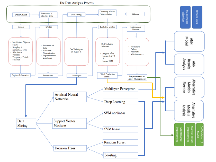
5. Employed DM Techniques

The employed DM techniques, for failure prediction, are presented below, using for comparison the mean square error to measure the quality of the results:
-
ANN Models:
Multilayer Perceptron
Deep Learning
-
Support Vector Machines:
SVM non-linear
SVM Lineal (Lib Linear)
-
Random Forest
-
Boosting
The practical implementation for each one of these techniques will now be introduced, describing the employed libraries, functions and transformation variables.
It is important to mention that unless learning is applied we cannot say that any DM model is intelligent. Therefore, for those situations when new data arrives after significant changes in an asset’s location or operation, a learning period for the algorithms is required.
The error predicted by the model can also offer a good clue regarding potential scenario modifications and can be used to trigger and lead to a new phase of model actualization, or learning period. This will reduce reasonable worries about model validation and will give more confidence to support asset managers’ decision-making regarding prediction and time estimation for the next failures. These ideas can also be programmed and automatically put into operation in the SCADA.

5.1. ANN Models: Multilayer Perceptron

For the case study, first, a three-layer perceptron is employed with the following activation functions: logistic and identity in the hidden layer (g(u) = eu/(eu + 1)) and in the output layer, respectively. If we denote wh synaptic weights between the hidden layer and the output layer {wh, h = 0, 1, 2, ..., H}, H as the size of the hidden layer, and vih synaptic weights of connections between the input layer (p size) and the hidden layer {vih, i = 0, 1, 2, …, p, h = 1, 2, …, H}, thus, with a vector of inputs (x1, …, xp), the output of the neural network could be represented by the following function (1):
o = w 0 + h = 1 H w h g ( v 0 h + i = 1 p v i h x i )
We have used the R library nnet [56], where multilayer perceptrons with one hidden layer are implemented. The nnet function needs, as parameters, the decay parameter (λ) to prevent overfitting in the optimization problem, and the size of the hidden layer (H). Therefore, providing the vector of all M coefficients of the neural net W = (W1, …, WM), and specified n targets y1, …, yn, the following optimization problem (Equation (2)) is (L2 regularization):
M i n W i = i n y i y ^ i 2 + λ ( i = i M W i 2 )
A quasi-Newton method, namely the BFGS (Broyden-Fletcher-Goldfarb-Shanno) training algorithm [44], is employed by nnet, in R with e1071 library using the tune function [57], determining the decay parameter (λ) as {1, 2, …, 15} × {0, 0.05, 0.1} by a ten-fold cross-validation search.
The λ parameter obtained for the two transformations presented below has been zero in all the models built, the logical value considering the sample size and the reduced number of predictor variables, which carries little risk of overfitting.
Through prior normalization of the input variables, the performance could be enhanced in the model. For that, we have considered two normalization procedures, a first transformation that subtracts each variable predictor X from its mean, and the centred variable is divided by the standard deviation of X. In this way we manage to normalize with a 0 mean and a standard deviation equal to 1. The second lineal normalization transforms the range of X values into the range (0, 1). We design, respectively, the values of the standards Z1 and Z2, which are calculated as follow:
Z 1 = X x ¯ s x Z 2 = X m i n x m a x x m i n x
These transformations have used the mean, standard deviation, maximums and minimums calculated in the network training dataset, and these same values have been used for the test set, thus avoiding the intervention of the test set in the training of the neural network.
Since the range of values provided by the logistic function is in the range (0, 1) and the dependent variable Y takes values in the range (0, 99). We transform this with the Y/100 calculation. However, after obtaining the predictions, the output values obtained in the original range were transformed back to the original range of values by multiplying by 100 to bring it back to the interval (0, 99).

5.2. ANN Models: Deep Learning

We have used the R package h2o [58] to prevent overfitting with several regularization terms, building a neural network with four layers, and with two hidden layers formed by 200 nodes each.
First, L1 and L2 regression terms are both included in the objective function to be minimized in the parameter estimation process (Equation (4)):
M i n W i = i n y i y ^ i 2 + λ 1 ( i = i M | W i | ) + λ 2 ( i = i M W i 2 )
Another regularization type to prevent overfitting is dropout, which averages a high number of models as a set with the same global parameters. In this type, during the training, in the forward propagation the activation of each neuron is supressed less than 0.2 in the input layer and up to 0.5 in the hidden layers, and provoking that weights of the network will be scaled towards 0.
The two normalization procedures used with nnet have also been used with h2o.

5.3. Alternative Models (SVM): Support Vector Machines (Non-Linear SVM)

Now, we have used the svm function of the R system library e1071 [57] for the development of the SVM models and, concretely, the ε-classification with the radial basis Gaussian kernel function (5); by n training compound vectors {xi, yi}, i = 1, 2, …, n as the dataset, where xi incorporates the predictor features and yi ∈ {−1, 1} are the results of each vector:
K ( u ,   v ) = exp ( γ u v 2 )
Therefore, it is solved by quadratic programming optimization (Equation (6)):
M i n w , b , ξ , ξ *   1 2 w t w + C i = 1 n ξ i + C i = 1 n ξ i * w t φ ( x i ) + b y i ε + ξ i y i w t φ ( x i ) + b ε + ξ i * w i t h   ξ i ,   ξ i * 0 ,   i = 1 , 2 , , n
With the parameter C > 0 to delimit the tolerated deviations from the desired ε accuracy. The additional slack variables ξ i ,   ξ i * allows the existence of points outside the ε-tube. The dual problem is given by Equation (7):
M i n α , α *   1 2 ( α α * ) t Q ( α α * ) + ε i = 1 n ( α i + α i * ) + y i i = 1 n ( α i α i * ) 0 α i , α i * C ,   i = 1 , 2 , , n i = 1 n ( α i α i * ) = 0
with K(xi, xj) = φ(xi)tφ(xj) being the kernel function, a positive semi-definite matrix Q is employed by Qij = K(xi, xj), i,j = 1, 2, …, n,. The prediction for a vector x (Equation (8)) is computed by:
i = 1 n ( α i + α i * ) K ( x i , x ) + b
depending on the margins m i = i = 1 n y i α i K ( x i , x ) + b , i = 1 , 2 , , n .
A cross-validation grid search for C and γ over the set {1, 5, 50, 100, 150, …, 1000} × {0.1, 0.2, 0.3, 0.4} was conducted by the R e1071 tune function, while the parameter ε was maintained at its default value, 0.1.
We have built this SVM model with the original input variables, and with the two normalization procedures previously described in the multilayer perceptron description.

5.4. Alternative Models (SVM): LibLineaR (Linear SVM)

A library for linear support vector machines is LIBLINEAR [59] for the case of large-scale linear prediction. We have used the version used in [60], with fast searching estimation (in comparison with other libraries) through the heuristicC function for C and based on the default values for ε, and employing L2-regularized support vector regression (with L1- and L2-loss).

5.5. Alternative Models (DT): Random Forests

The Random Forests (RF) algorithm [61] combines different predictor trees, each one fitted on a bootstrap sample of the training dataset. Each tree is grown by binary recursive partitioning, where each split is determined by a search procedure aimed to find the variable of a partition rule which provides the maximum reduction in the sum of the squared error. This process is repeated until the terminal nodes are too small to be partitioned. In each terminal node, the average of response variable is the prediction. RF is similar to bagging [39], with an important difference: the search for each split is limited to a random selection of variables, improving the computational cost. We have used the R package Random Forest [62]. By default, p/3 variables (p being the predictor’s number) are randomly selected in each split, and 500 trees are grown.

5.6. Alternative Models (DT): Boosting

From the different boosting models depending on the used loss functions, base models, and optimization schemes, we have employed one based on Friedman´s gradient boosting machine of the R gbm package [63] where the target is to boost the performance of a single tree with the following parameters:
-
The squared error as a loss function ψ (distribution),
-
T (n.trees) as the number of iterations,
-
The depth of each tree, K (interaction.depth),
-
The learning rate parameter, λ (shrinkage), and
-
The subsampling rate, p (bag.fraction).
The function f ^ ( x ) = arg   m i n ρ i = 1 n ψ ( y i , ρ ) is initialized to be a constant. For t in 1, 2, …, T do the following:
  • Compute the negative gradient as the working response:
    z i = f ( x i ) ψ ( y i , f ( x i ) ) | f ( x i ) = f ^ ( x i )
  • Randomly select pxn cases from the dataset.
  • Fit a regression tree with K terminal nodes and using only those randomly selected observations.
  • Compute the optimal terminal node predictions ρ 1 , …, ρ k , as:
    ρ k = arg   m i n ρ x i ϵ S k ψ ( y i , f ^ ( x i ) + ρ )
    where Sk is the set of cases that define terminal node k, using again only the randomly selected observations.
  • Update f ^ ( x ) as:
    f ^ ( x ) = f ^ ( x ) + λ ρ k ( x )
    where k(x) indicates the index of the terminal node into which an observation with features x would fall.
Following the suggestions of Ridgeway in his R package, our work considered the following values:
shrinkage = 0.001; bag.fraction = 0.5; interaction.depth = 4; n.trees = 5000, but cv.folds 10 performed a cross-validation search for the effective number of trees.

6. Results

The obtained results for each technique are shown below (Table 5), as well as the different transformations made (different ways to normalize variables and to estimate parameters), shading in each technique the one that gives us the best solution.
We graphically represent (Figure 5) the best result obtained for each of the techniques in order to visualize the one that gives us the best solution for the behaviour pattern of the production of the photovoltaic installation.
A point cloud chart (Figure 6) of the predicted (test) production is shown for the model that give us the best solution (Random Forest).
This model tells us the importance of variables in the result, which shows that all of them are valid and necessary. The higher the percentage, the higher the importance variable (see Table 6).
The prediction error based on %INC_MSE is estimated by out-of-bag (OOB) for each tree and after permuting each predictor variable, until the difference between them has a standard deviation equal to 0.

7. Conclusions

In this paper a methodology to introduce the use of different data mining techniques for energy forecasting and condition-based maintenance was followed. These techniques compete for the best possible replica of the production behaviour patterns.
A relevant set of DM techniques have been applied (ANN, SVM, DT), and after their introduction to the readers, they were compared when applied to a renewable energy (PV installation) case study.
In this paper a very large sample of data has been considered. This data spans from 1 June 2011 to 30 September 2015.
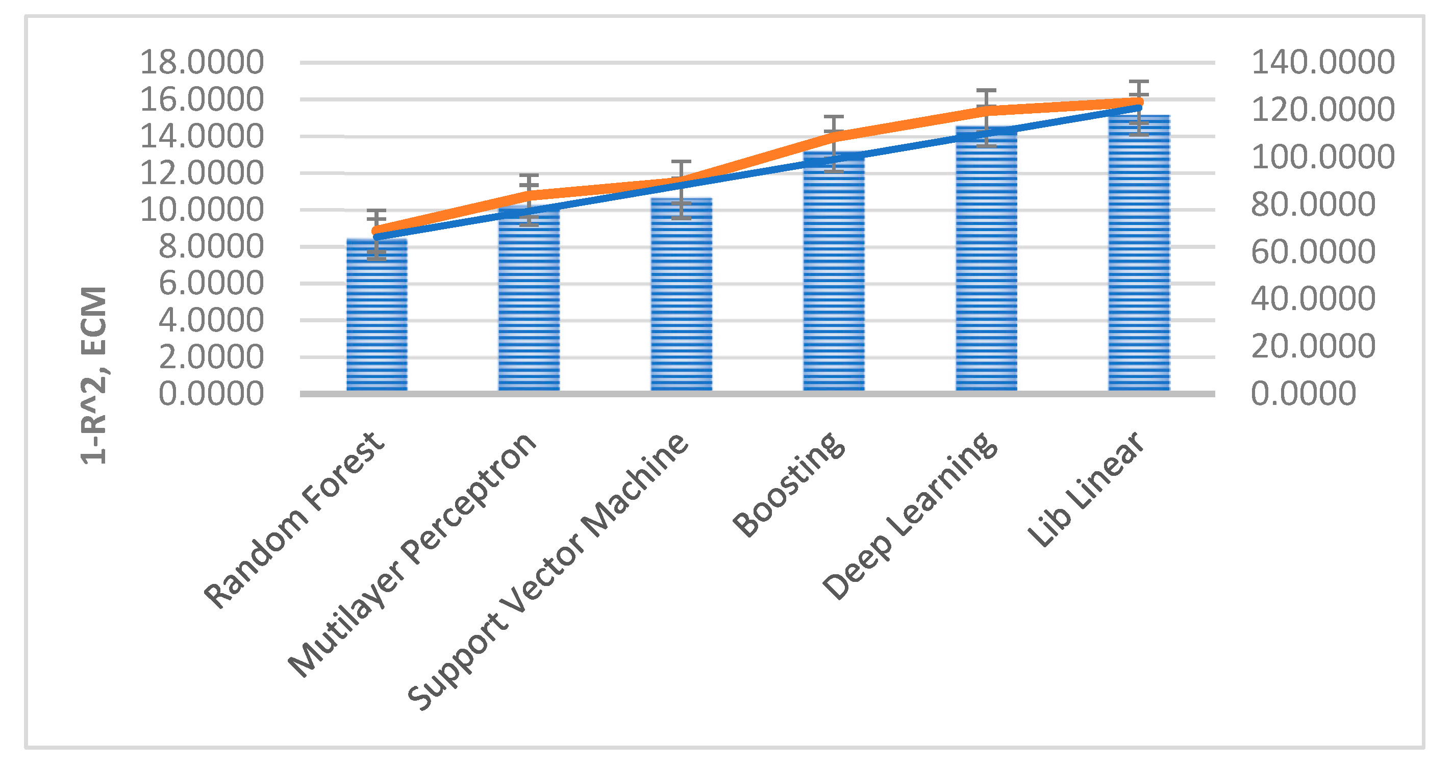
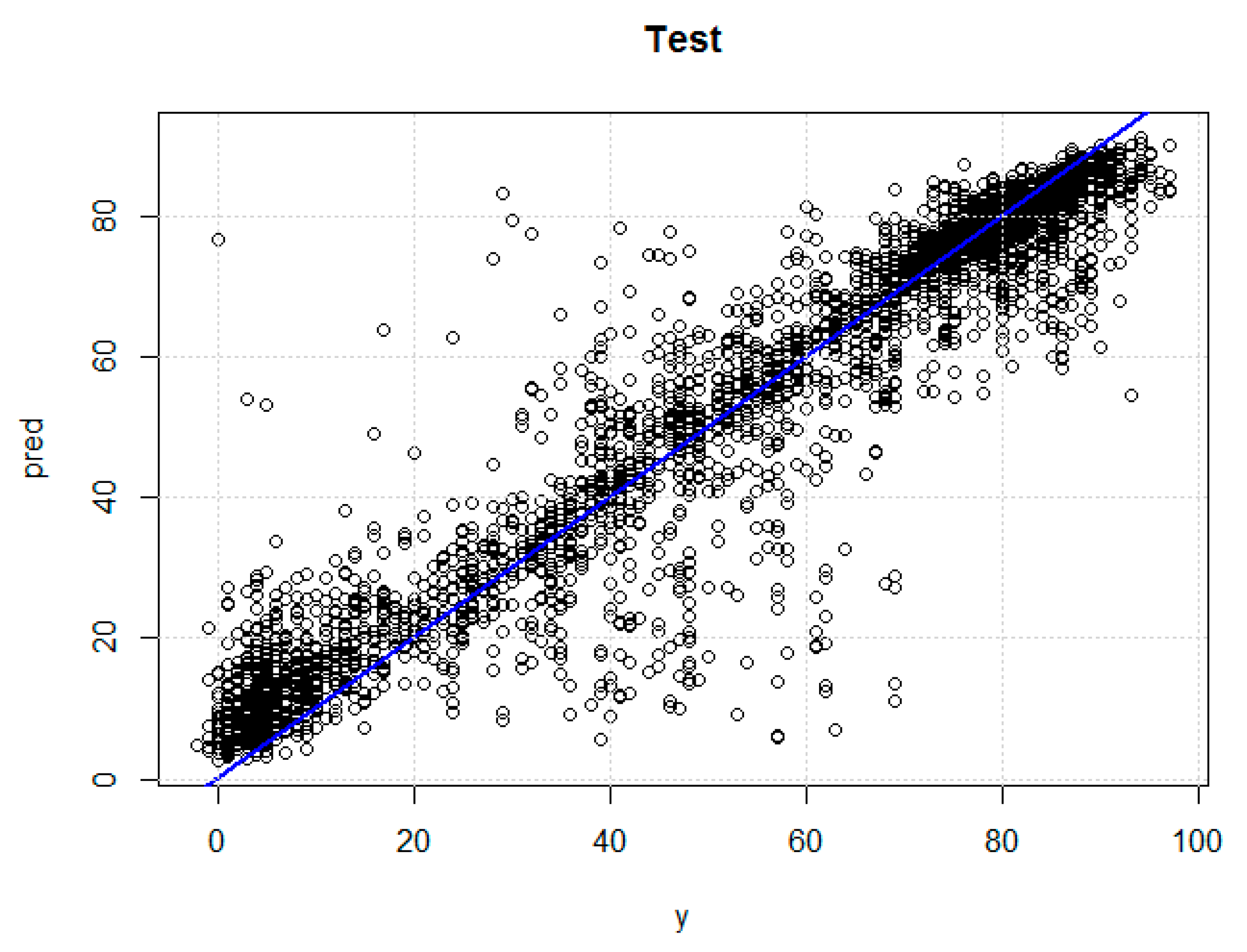
All of the models for the different techniques offered very encouraging results, with correlation coefficients greater than 0.82. Coincident with other referenced authors’ results, Random Forest was the technique providing the best fit, with a linear correlation coefficient of 0.9092 (followed by ANN and SVM). In turn, this technique (RF) gave us as a differential value of the importance of the input variables used in the model, which somehow validates the use of all these variables. In the case study, and by far, the variable resulting with the most affection to production was radiation, followed by the outside temperature, the inverter internal temperature and, finally, the operating hours (which somehow reflects the asset degradation over time).
It is important to mention that these results were obtained using different methods (2) to normalize the variables and to estimate parameters.
Future work could be devoted to the validation of these results by replicating the study at other renewable energy facilities to determine how the improvement in ECM and R2 values affects early detection of failures by quantifying their economic value.
The implementation of these techniques is feasible today thanks to existing computational capacity, so the effort to use any of them is very similar.

Author Contributions

Conceptualization: J.F.B., J.F.G.F. and A.C.M.; methodology: J.F.B. and J.F.G.F.; software: R.P.; validation, R.P. and J.F.B.; formal analysis: J.F.B. and J.F.G.F.; investigation: J.F.B.; resources, J.F.B.; data curation, J.F.B.; writing—original draft preparation, J.F.B. and A.C.M.; writing—review and editing, A.J.G.L.; supervision, J.F.G.F. and A.C.M.; project administration: A.C.M.; funding acquisition A.C.M.

Funding

This project: Intelligent Assets Management Systems (ES-1794/44/2018) is funded by INGEMAN Association for Maintenance Engineering Development.

Conflicts of Interest

The authors declare no conflict of interest.

Acronyms

ANNArtificial neural networks
CBMCondition-based maintenance
DMData mining
DPDeep learning
DTDecision trees
IDAIntelligent data analysis
IoTInternet of Things
MPMultilayer perceptron
MSEMean square error
OOBOut-of-Bag
PBMPhysics-based model
PdMPredictive maintenance
PHMPrognostics and health management
POFPhysics of failure
PVPhotovoltaic
RMSERoot mean square error
RFRandom Forest
ROIReturn on investment
RSVMGRecurrent support vector model
RULRemaining useful life forecast
SCADASupervisory control and data acquisition
SVMSupport vector machine
SVRSupport vector regression

References

  1. Shin, Y.C.; Xu, C. Intelligent Systems: Modeling, Optimization, and Control; CRC Press: Boca Raton, FL, USA, 2017. [Google Scholar]
  2. IIC-Industrial Internet Consortium. The Industrial Internet of Things, Volume B01: Business Strategy and Innovation Framework (IIC: PUB: B01: V1. 0: PB: 20161115). Available online: http://www. iiconsortium org/pdf/Business_Strategy_and_Innovation_Framework_Nov_2016 pdf (accessed on 8 November 2016).
  3. Barton, D.; Court, D. Making advanced analytics work for you. Harv. Bus. Rev. 2012, 90, 78–83. [Google Scholar]
  4. Chau, K.W. Kwok-wing Chau Integration of Advanced Soft Computing Techniques in Hydrological Predictions. Atmosphere 2019, 10, 101. [Google Scholar] [CrossRef]
  5. Fayyad, U.M.; Piatetsky-Shapiro, G.; Smyth, P. Knowledge Discovery and Data Mining: Towards a Unifying Framework. KDD 1996, 96, 82–88. [Google Scholar]
  6. Clarke, R. Big data, big risks. Inf. Syst. J. 2016, 26, 77–90. [Google Scholar] [CrossRef]
  7. Polo, F.A.O.; Bermejo, J.F.; Fernández, J.F.G.; Márquez, A.C. Failure mode prediction and energy forecasting of PV plants to assist dynamic maintenance tasks by ANN based models. Renew. Energy 2015, 81, 227–238. [Google Scholar] [CrossRef]
  8. Mellit, A.; Benghanem, M.; Kalogirou, S.A. Modeling and simulation of a stand-alone photovoltaic system using an adaptive artificial neural network: Proposition for a new sizing procedure. Renew. Energy 2007, 32, 285–313. [Google Scholar] [CrossRef]
  9. Piatetsky-Shapiro, G. Advances in Knowledge Discovery and Data Mining; Fayyad, U.M., Smyth, P., Uthurusamy, R., Eds.; AAAI Press: Menlo Park, CA, USA, 1996; Volume 21. [Google Scholar]
  10. Berthold, M.R.; Hand, D.J. (Eds.) Intelligent Data Analysis: An Introduction; Springer: Berlin, Germany, 2007. [Google Scholar]
  11. Guillén, A.J.; Crespo, A.; Gómez, J.F.; Sanz, M.D. A framework for effective management of condition based maintenance programs in the context of industrial development of E-Maintenance strategies. Comput. Ind. 2016, 82, 170–185. [Google Scholar] [CrossRef]
  12. Banos, R.; Manzano-Agugliaro, F.; Montoya, F.G.; Gil, C.; Alcayde, A.; Gómez, J. Optimization methods applied to renewable and sustainable energy: A review. Renew. Sustain. Energy Rev. 2011, 15, 1753–1766. [Google Scholar] [CrossRef]
  13. Kusiak, A.; Verma, A. A data-mining approach to monitoring wind turbines. IEEE Trans. Sustain. Energy 2012, 3, 150–157. [Google Scholar] [CrossRef]
  14. Antonanzas, J.; Osorio, N.; Escobar, R.; Urraca, R.; Martinez-de-Pison, F.J.; Antonanzas-Torres, F. Review of photovoltaic power forecasting. Sol. Energy 2016, 136, 78–111. [Google Scholar] [CrossRef]
  15. Mellit, A.; Pavan, A.M. A 24-h forecast of solar irradiance using artificial neural network: Application for performance prediction of a grid-connected PV plant at Trieste, Italy. Sol. Energy 2010, 84, 807–821. [Google Scholar] [CrossRef]
  16. Rehman, S.; Mohandes, M. Artificial neural network estimation of global solar radiation using air temperature and relative humidity. Energy Policy 2008, 36, 571–576. [Google Scholar] [CrossRef] [Green Version]
  17. Mabel, M.C.; Fernandez, E. Analysis of wind power generation and prediction using ANN: A case study. Renew. Energy 2008, 33, 986–992. [Google Scholar] [CrossRef]
  18. Kusiak, A.; Zhang, Z.; Verma, A. Prediction, operations, and condition monitoring in wind energy. Energy 2013, 60, 1–12. [Google Scholar] [CrossRef]
  19. Coulibaly, P.; Anctil, F.; Bobee, B. Daily reservoir inflow forecasting using artificial neural networks with stopped training approach. J. Hydrol. 2000, 230, 244–257. [Google Scholar] [CrossRef]
  20. Dawson, C.W.; Wilby, R. An artificial neural network approach to rainfall-runoff modelling. Hydrol. Sci. J. 1998, 43, 47–66. [Google Scholar] [CrossRef]
  21. Voyant, C.; Notton, G.; Kalogirou, S.; Nivet, M.L.; Paoli, C.; Motte, F.; Fouilloy, A. Machine learning methods for solar radiation forecasting: A review. Renew. Energy 2017, 105, 569–582. [Google Scholar] [CrossRef]
  22. Li, Z.; Rahman, S.M.; Vega, R.; Dong, B. A hierarchical approach using machine learning methods in solar photovoltaic energy production forecasting. Energies 2016, 9, 55. [Google Scholar] [CrossRef]
  23. Hooman, A.; Marthandan, G.; Yusoff, W.F.W.; Omid, M.; Karamizadeh, S. Statistical and data mining methods in credit scoring. J. Dev. Areas 2016, 50, 371–381. [Google Scholar] [CrossRef]
  24. Moreno-Sáez, R.; Mora-López, L. Modelling the distribution of solar spectral irradiance using data mining techniques. Environ. Model. Softw. 2014, 53, 163–172. [Google Scholar] [CrossRef]
  25. Minemoto, T.; Nakada, Y.; Takahashi, H.; Takakura, H. Uniqueness verification of solar spectrum index of average photon energy for evaluating outdoor performance of photovoltaic modules. Sol. Energy 2009, 83, 1294–1299. [Google Scholar] [CrossRef]
  26. Mellit, A.; Kalogirou, S.A. Artificial intelligence techniques for photovoltaic applications: A review. Prog. Energy Combust. Sci. 2008, 34, 574–632. [Google Scholar] [CrossRef]
  27. Kalogirou, S.A. Artificial neural networks in renewable energy systems applications: A review. Renew. Sustain. Energy Rev. 2011, 5, 373–401. [Google Scholar] [CrossRef]
  28. Kalogirou, S.A.; Bojic, M. Artificial neural networks for the prediction of the energy consumption of a passive solar building. Energy 2000, 25, 479–491. [Google Scholar] [CrossRef]
  29. Renno, C.; Petito, F.; Gatto, A. Artificial neural network models for predicting the solar radiation as input of a concentrating photovoltaic system. Energy Convers. Manag. 2016, 106, 999–1012. [Google Scholar] [CrossRef]
  30. Polson, N.G.; Sokolov, V.O. Deep learning for short-term traffic flow prediction. Transp. Res. Part C Emerg. Technol. 2017, 79, 1–17. [Google Scholar] [CrossRef] [Green Version]
  31. Wang, H.Z.; Li, G.Q.; Wang, G.B.; Peng, J.C.; Jiang, H.; Liu, Y.T. Deep learning based ensemble approach for probabilistic wind power forecasting. Appl. Energy 2017, 188, 56–70. [Google Scholar] [CrossRef]
  32. Li, C.; Bai, Y.; Zeng, B. Deep Feature Learning Architectures for Daily Reservoir Inflow Forecasting. Water Resour. Manag. 2016, 30, 5145–5161. [Google Scholar] [CrossRef]
  33. Li, Q.; Meng, Q.; Cai, J.; Yoshino, H.; Mochida, A. Predicting hourly cooling load in the building: A comparison of support vector machine and different artificial neural networks. Energy Convers. Manag. 2009, 50, 90–96. [Google Scholar] [CrossRef]
  34. Chen, J.L.; Liu, H.B.; Wu, W.; Xie, D.T. Estimation of monthly solar radiation from measured temperatures using support vector machines—A case study. Renew. Energy 2011, 36, 413–420. [Google Scholar] [CrossRef]
  35. Zhang, H.; Chen, L.; Qu, Y.; Zhao, G.; Guo, Z. Support vector regression based on grid-search method for short-term wind power forecasting. J. Appl. Math. 2014, 2014, 1–11. [Google Scholar] [CrossRef]
  36. Shi, J.; Lee, W.J.; Liu, Y.; Yang, Y.; Wang, P. Forecasting power output of photovoltaic systems based on weather classification and support vector machines. IEEE Trans. Ind. Appl. 2012, 48, 1064–1069. [Google Scholar] [CrossRef]
  37. Pai, P.F.; Hong, W.C. A recurrent support vector regression model in rainfall forecasting. Hydrol. Process. 2007, 21, 819–827. [Google Scholar] [CrossRef]
  38. Benedetti, M.; Cesarotti, V.; Introna, V.; Serranti, J. Energy consumption control automation using Artificial Neural Networks and adaptive algorithms: Proposal of a new methodology and case study. Appl. Energy 2016, 165, 60–71. [Google Scholar] [CrossRef]
  39. Elyan, E.; Gaber, M.M. A genetic algorithm approach to optimising random forests applied to class engineered data. Inf. Sci. 2017, 384, 220–234. [Google Scholar] [CrossRef]
  40. Lin, Y.; Kruger, U.; Zhang, J.; Wang, Q.; Lamont, L.; El Chaar, L. Seasonal analysis and prediction of wind energy using random forests and ARX model structures. IEEE Trans. Control Syst. Technol. 2015, 23, 1994–2002. [Google Scholar] [CrossRef]
  41. Moutis, P.; Skarvelis-Kazakos, S.; Brucoli, M. Decision tree aided planning and energy balancing of planned community microgrids. Appl. Energy 2016, 161, 197–205. [Google Scholar] [CrossRef] [Green Version]
  42. Ren, L.; Hartnett, M. Prediction of Surface Currents Using High Frequency CODAR Data and Decision Tree at a Marine Renewable Energy Test Site. Energy Procedia 2017, 107, 345–350. [Google Scholar] [CrossRef]
  43. Brillante, L.; Gaiotti, F.; Lovat, L.; Vincenzi, S.; Giacosa, S.; Torchio, F.; Tomasi, D. Investigating the use of gradient boosting machine, random forest and their ensemble to predict skin flavonoid content from berry physical-mechanical characteristics in wine grapes. Comput. Electron. Agric. 2015, 117, 186–193. [Google Scholar] [CrossRef]
  44. Bishop, C.M. Neural Networks for Pattern Recognition; Oxford University Press: Oxford, UK, 1995. [Google Scholar]
  45. Boser, B.E.; Guyon, I.M.; Vapnik, V.N. A training algorithm for optimal margin classifiers. In Proceedings of the Fifth Annual Workshop on Computational Learning Theory, Pittsburgh, PA, USA, 27–29 July 1992; pp. 144–152. [Google Scholar]
  46. Jardine, A.K.; Lin, D.; Banjevic, D. A review on machinery diagnostics and prognostics implementing condition-based maintenance. Mech. Syst. Signal Process. 2006, 20, 1483–1510. [Google Scholar] [CrossRef]
  47. Xiao, D.; Chang, M.C.; Niu, Q. Berry phase effects on electronic properties. Rev. Mod. Phys. 2010, 82, 1959. [Google Scholar] [CrossRef]
  48. González-Prida Díaz, V.; Barberá Martínez, L.; Gómez Fernández, J.F.; Crespo Márquez, A. Contractual and quality aspects on warranty: Best practices for the warranty management and its maturity assessment. Int. J. Qual. Reliab. Manag. 2012, 29, 320–348. [Google Scholar] [CrossRef]
  49. Vachtsevanos, G.J.; Lewis, F.; Hess, A.; Wu, B. Intelligent Fault Diagnosis and Prognosis for Engineering Systems; Wiley: Hoboken, NJ, USA, 2006; Volume 456. [Google Scholar]
  50. Lee, J.; Ghaffari, M.; Elmeligy, S. Self-maintenance and engineering immune systems: Towards smarter machines and manufacturing systems. Ann. Rev. Control 2011, 35, 111–122. [Google Scholar] [CrossRef]
  51. Zio, E. Some challenges and opportunities in reliability engineering. IEEE Trans. Reliab. 2016, 65, 1769–1782. [Google Scholar] [CrossRef]
  52. Zio, E. Reliability engineering: Old problems and new challenges. Reliab. Eng. Syst. Saf. 2009, 94, 125–141. [Google Scholar] [CrossRef] [Green Version]
  53. Jaw, L.C.; Merrill, W. CBM+ research environment-facilitating technology development, experimentation, and maturation. In Proceedings of the 2008 IEEE Aerospace Conference, Big Sky, MT, USA, 1–8 March 2008; IEEE: Piscataway, NJ, USA, 2008; pp. 1–6. [Google Scholar]
  54. Seuring, S.; Müller, M. From a literature review to a conceptual framework for sustainable supply chain management. J. Clean. Prod. 2008, 16, 1699–1710. [Google Scholar] [CrossRef]
  55. Lee, J.; Bagheri, B.; Kao, H.A. A cyber-physical systems architecture for industry 4.0-based manufacturing systems. Manuf. Lett. 2015, 3, 18–23. [Google Scholar] [CrossRef]
  56. Venables, W.N.; Ripley, B.D. Random and mixed effects. In Modern Applied Statistics with S.; Springer: New York, NY, USA, 2002; pp. 271–300. [Google Scholar]
  57. Meyer, D.; Dimitriadou, E.; Hornik, K.; Weingessel, A.; Leisch, F. e1071: Misc Functions of the Department of Statistics, Probability Theory Group (Formerly: E1071); R Package Version 1.6–7; TU Wien: Wien, Austria, 2017. [Google Scholar]
  58. Landry, M.; Angela, B. Machine Learning with R and H2O; H2O.ai: Mountain View, CA, USA, 2016. [Google Scholar]
  59. Fran, R.E.; Chang, D.K.; Hsieh, C.J.; Wang, X.R.; Lin, Y.C.J. LIBLINEAR: Una biblioteca para la Clasificación grande lineal. J. Mach. Learn. Investig. 2008, 9, 1871–1874. [Google Scholar]
  60. Helleputte, T.; Gramme, P. LiblineaR: Linear Predictive Models Based on the LIBLINEAR C/C++ Library. R Package Version, 2–10. 2017. Available online: https://rdrr.io/cran/LiblineaR/ (accessed on 29 October 2019).
  61. Breiman, L. Random forests. Mach. Learn. 2001, 45, 5–32. [Google Scholar] [CrossRef]
  62. Liaw, A.; Wiener, M. Classification and regression by random Forest. R News 2002, 2, 18–22. [Google Scholar]
  63. Ridgeway, G. The gbm Package. Generalized Boosted Regression Models (Documentation on the R Package ‘Gbm’, Version 1.6–3). 2015. Available online: https://rdrr.io/cran/gbm/man/gbm.html (accessed on 29 October 2019).
Figure 1. IDA phases for a renewable energy case study [9,10].
Energies 12 04163 g001
Figure 2. Predictive technique type classification [14].
Energies 12 04163 g002
Figure 3. Classification of DM techniques included in this paper.
Energies 12 04163 g003
Figure 4. Methodology for using alternative DM techniques.
Energies 12 04163 g004
Figure 5. Graphical comparison of the different techniques results.
Energies 12 04163 g005
Figure 6. Point cloud (test) Random Forest.
Energies 12 04163 g006
Table 1. References of DM techniques analysed.
TechniquesReferences
Data mining[13,21,22,23,24,25]
Artificial neural networks[7,26,27,28,29,30,31,32]
Support vector machine[33,34,35,36,37]
Decision trees[14,21,38,39,40,41,42,43]
Table 2. Temporary period for data collection for study.
Start DateEnd DateData CollectionFromUntilFrequency
01/06/201130/09/2015Hourly8:0017:0010 daily data for each variable
Table 3. Selected variables/data for training and validation.
Inputs VariablesOutputs VariablesSelected ValuesTraining Set PercentageTesting Set Percentage
Outdoor temperature, radiation, inside inverter temperature, operation hoursTime, productionIn the absence of failures75%25%
Same criteria for all techniques in order to establish the same comparison environment
Table 4. Collected data in the study (treated and validated).
Outdoor TempRadiationIndoor TempOperating TimeProduction
303.25490.3312.1990052
313.25756.0311990174
319.25860.8314.7990280
323.25901.8313.9990382
325.25918.0315.5990483
327.98990.3316.825,71681
320.77520.0315.625,71753
311.43454.5317.125,71839
305.98777.3317.825,71966
Table 5. Results of the different techniques.
Models AnalysisResults
Multilayer PerceptronTransformation 1Coefficient CorrelationRMSE
Test0.8869.64
Training0.8979.15
Transformation 2Coefficient CorrelationRMSE
Test0.8839.76
Training0.8959.26
Deep LearningTransformation 1Coefficient CorrelationRMSE
Test0.83911.5
Training0.85510.93
Transformation 2Coefficient CorrelationRMSE
Test0.83811.72
Training0.85311.19
SVM NonlinearTransformation 1, 2 and 3Coefficient CorrelationRMSE
Test0.88110.01
Training0.8949.46
SVM Linear (Lib Linear)Transformation 1Coefficient CorrelationRMSE
Test0.83611.57
Training0.84811.1
Transformation 2Coefficient CorrelationRMSE
Test0.82113.54
Training0.83413.07
Random Forest Coefficient CorrelationRMSE
Test0.9098.63
Training0.9168.3
Boosting Coefficient CorrelationRMSE
Test0.85610.87
Training0.86810.41
Table 6. Importance of the variables.
VARIABLE% INC_MSE
TEMP_EXT49.10
RADIACIÓN155.63
TEMP_INT41.60
H. FUNCIONAMIENTO34.37

