Energy Balanced Localization-Free Cooperative Noise-Aware Routing Protocols for Underwater Wireless Sensor Networks


Abstract
:1. Introduction
1.1. Motivation
1.2. Contributions
2. Channel Model
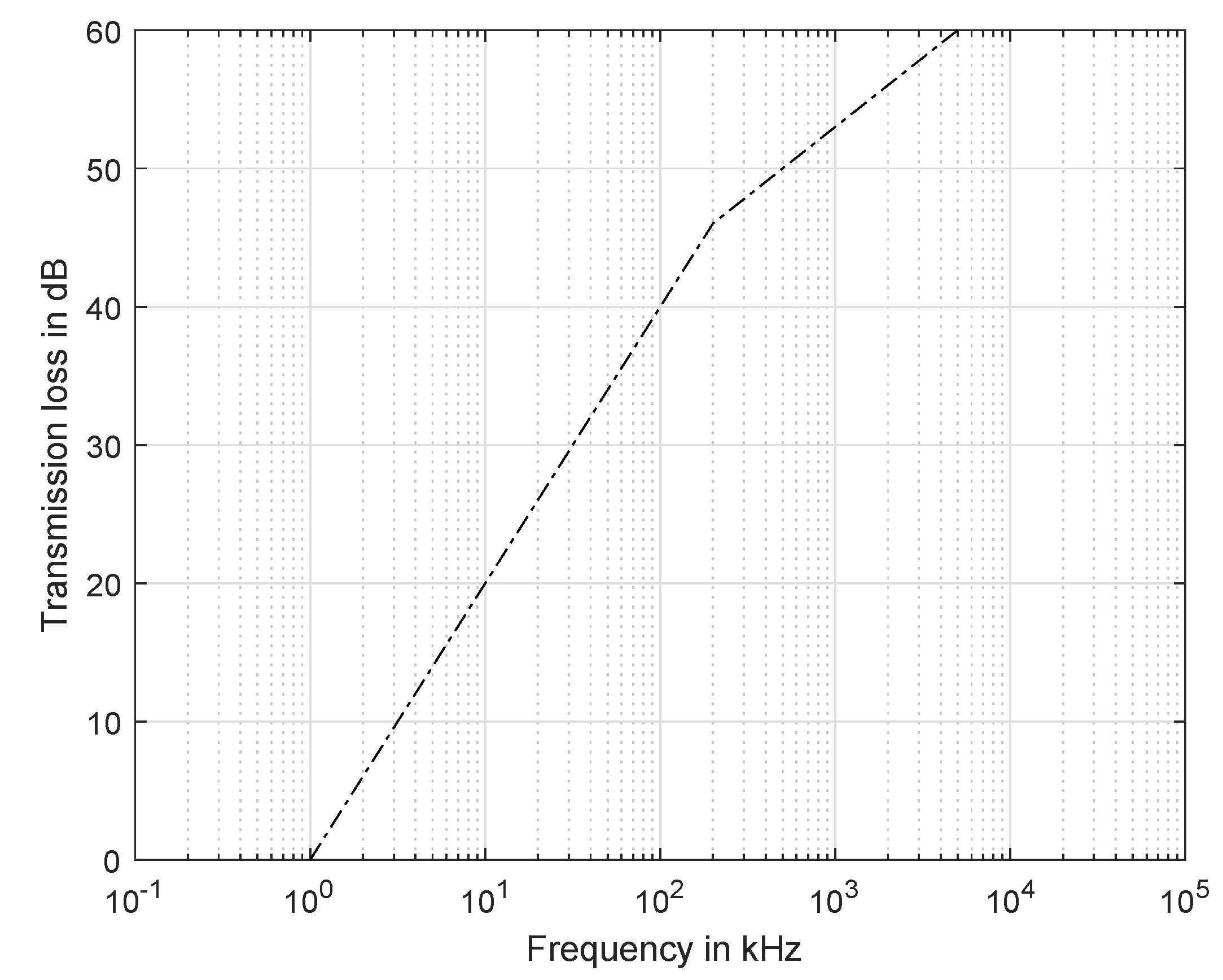
2.1. Transmission Loss
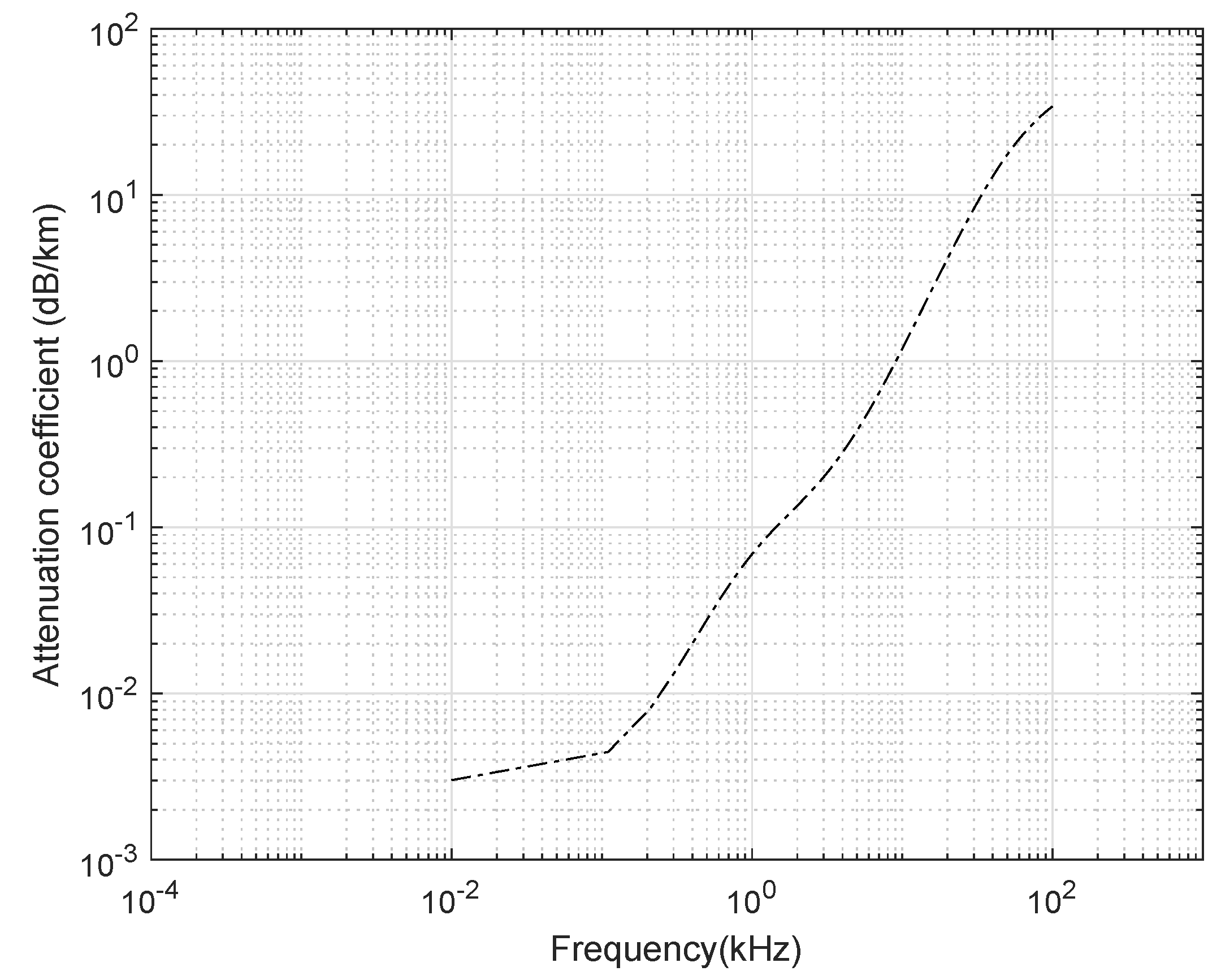
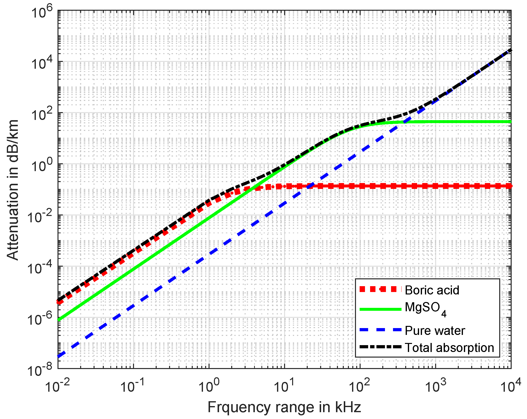
2.2. Channel Attenuation
2.3. Speed of Sound
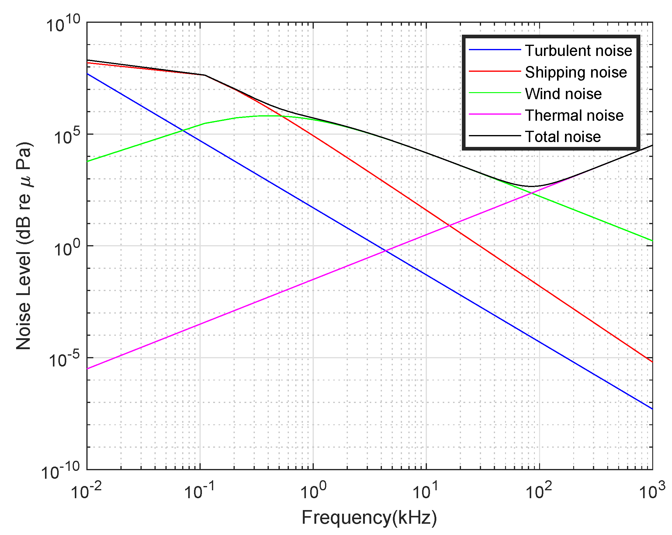
2.4. Channel Noise
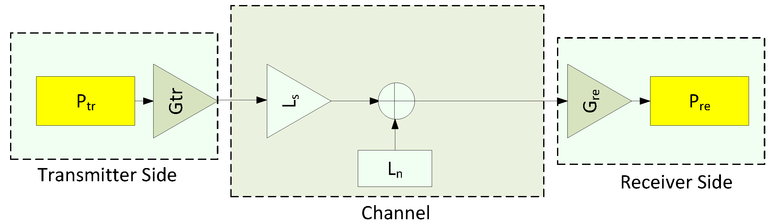
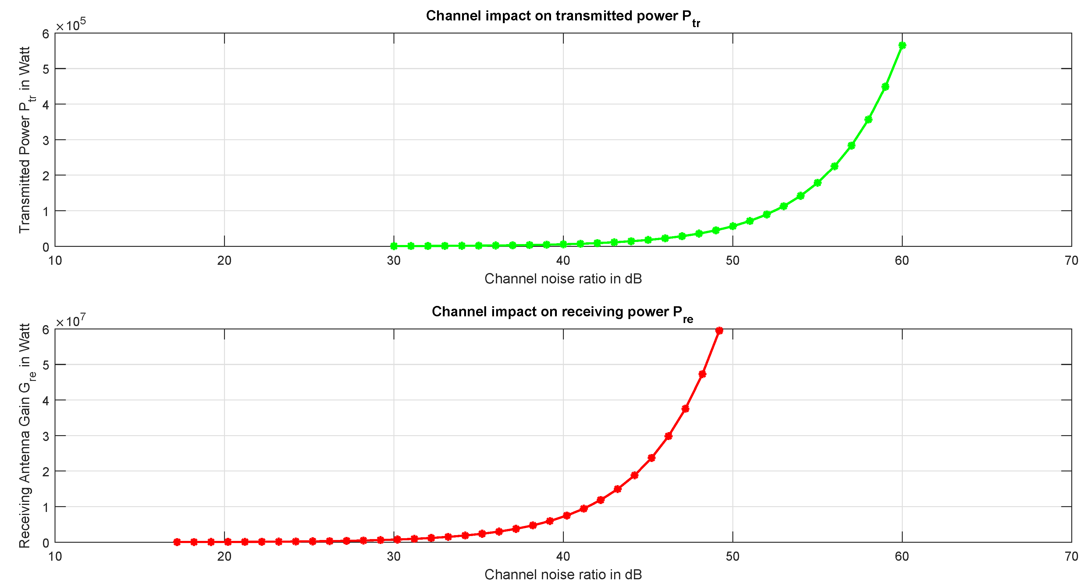
2.5. Link Budget
2.6. Sleeping Scheduling Energy Calculation
2.7. Absorption
3. Proposed Protocol: Co-DNAR
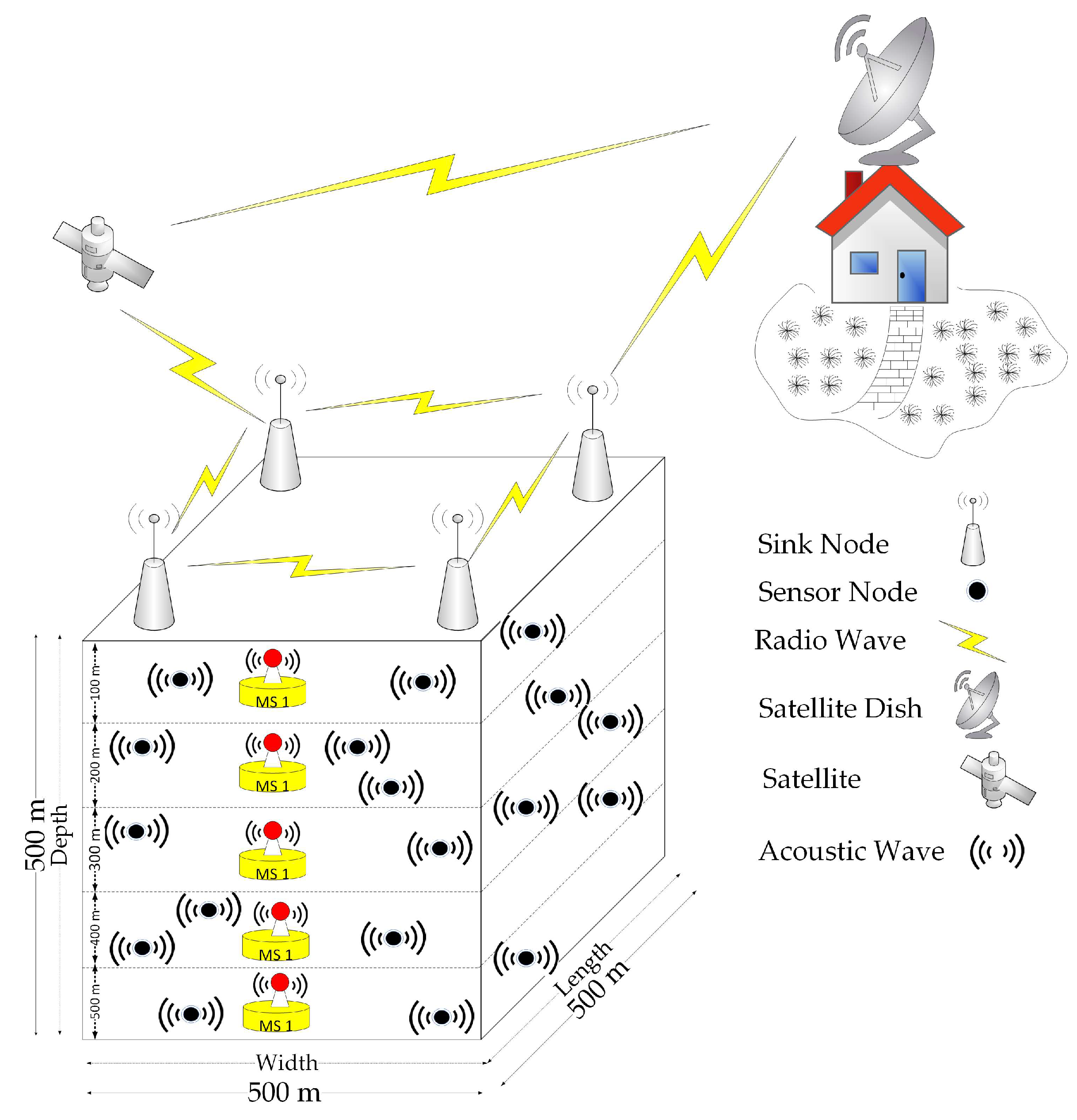
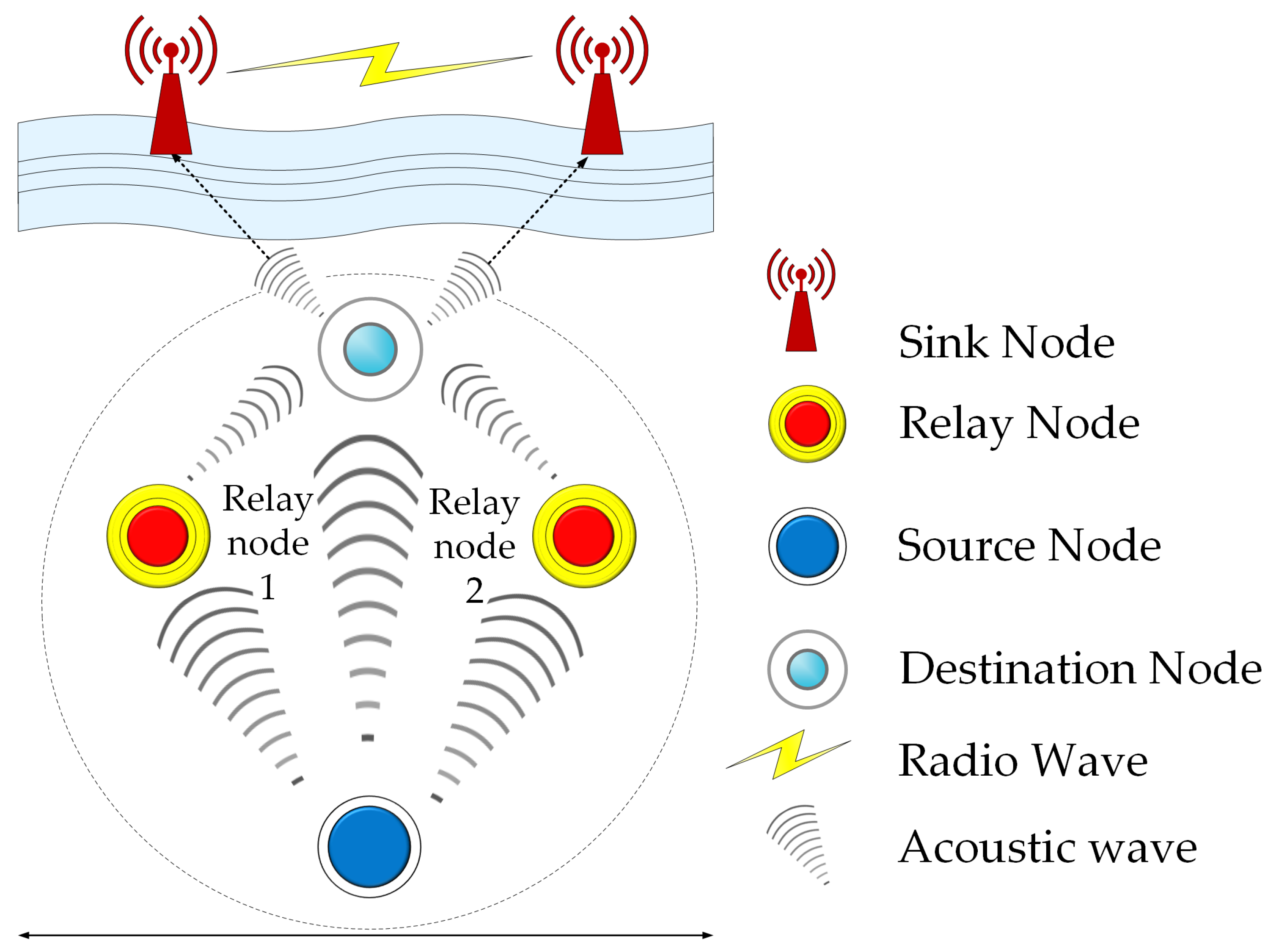
3.1. Network Settings
3.2. Neighbours Identification
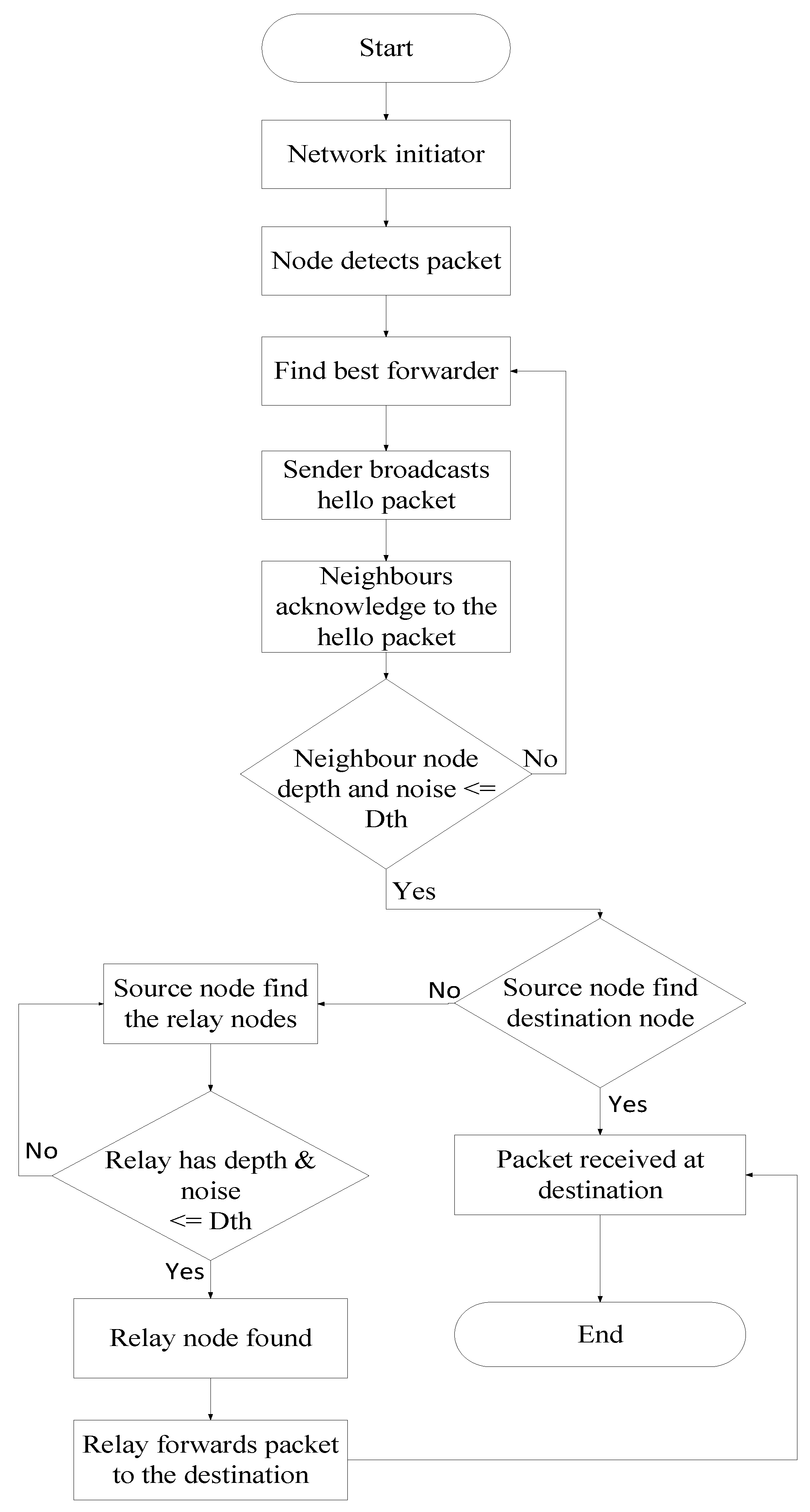
3.3. Data Forwarding
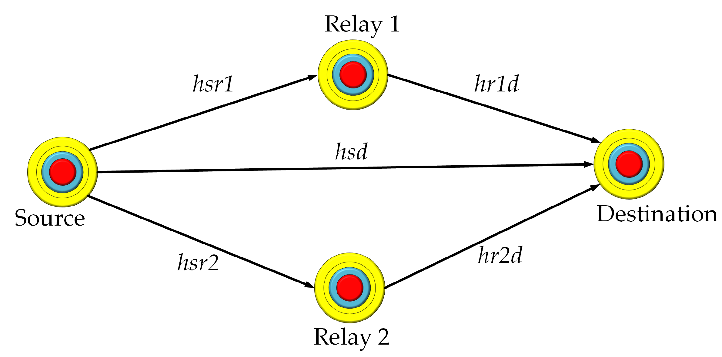
3.4. Cooperation of Relay Nodes
| Algorithm 1: Data Cooperation. |
| The best relay node Sink Surface Sender node Receiving node Depth of the sensor node i Neighbour of the source node i for i = 1 : 1 : S do BR forwards a data packet while(data packet not reached(to the SS)) do if = then if BER < Threshold then packet accepted find neighbours N Sort the depth of N neighbours in ascending order else if Make as 1st relay node Make as 2nd relay node Packets reached to the = True while packets not reached to the else Packets drop end if else Nodes consume all of the energy and have no battery power end while end if end for |
3.5. Combining Diversity Technique
4. Proposed Protocol: DNAR
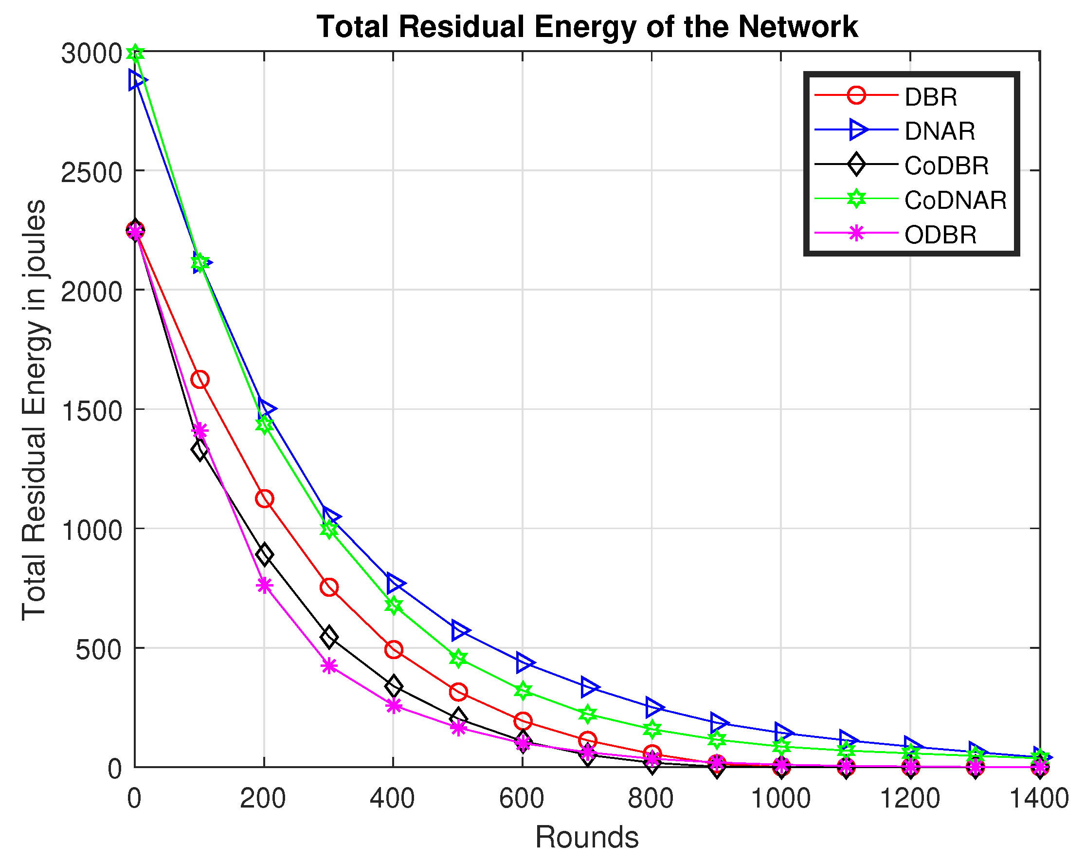
5. Simulation Settings
6. Conclusions and Future Work
Author Contributions
Funding
Conflicts of Interest
Abbreviations
| AF | Amplify and forward |
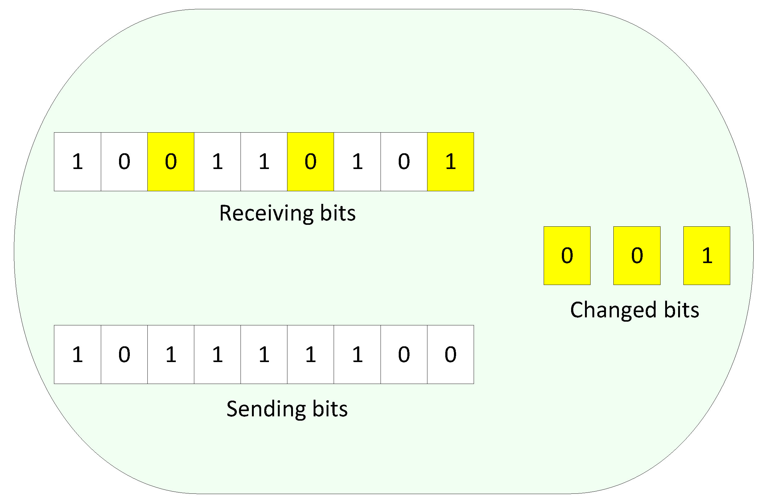
| BER | Bit error rate |
| dB | Decibel |
| FLRS | Fuzzy logic relay selection |
| MSs | Mobile sinks |
| MAC | Medium access control |
| MRC | Maximal combining ratio |
| PSD | Power spectral density |
| UWSNs | Underwater wireless sensor networks |
References
- Ahmad, A.; Ahmed, S.; Imran, M.; Alam, M.; Niaz, I.A.; Javaid, N. On energy efficiency in underwater wireless sensor networks with cooperative routing. Ann. Telecommun. 2017, 72, 1730188. [Google Scholar] [CrossRef]
- Paola, N.; Vinueza, G.; Shojafar, M.; Mostafai, H.; Pooramian, Z.; Baccarelli, E. P-SEP: A prolong stable election routing algorithm for energy-limited heterogenous fog-supported wireless sensor networks. J. Supercomput. 2017, 73, 733–755. [Google Scholar]
- Jiang, J.; Han, G.; Guo, H.; Shu, L.; Jpc, J. Geographic mulitpath routing based on geospatial division in duty-cycled underwater wireless sensor networks. J. Netw. Comput. Appl. 2016, 59, 4–13. [Google Scholar] [CrossRef]
- Ullah, U.; Anwar, K.; Mahdi, Z.; Ihsan, A.; Hasan, A.K.; Ikram, U.D. Energy-Effective Cooperative and Reliable Delivery Routing Protocols for Underwater Wireless Sensor Networks. Energies 2019, 12, 2630. [Google Scholar] [CrossRef]
- Khosravi, M.R.; Basri, H.; Khosravi, A.; Rostami, H. Energy efficient spherical divisions for VBF-based routing in dense UWSNs. In Proceedings of the 2015 2nd International Conference on Knowledge-Based Engineering and Innovation (KBEI), Tehran, Iran, 5–6 November 2015; pp. 961–965. [Google Scholar]
- Coutinho, R.W.L.; Azzedine, B.; Vieira, L.F.M.; Loureiro, A.A.F. Underwater Wireless Sensor Networks: A New Challenge for Topology Control–Based Systems. ACM Comput. Surv. (CSUR) 2018, 51, 19. [Google Scholar] [CrossRef]
- Poncela, J.; Aguayo, M.C.; Otero, P. Wireless underwater communications. Wirel. Pers. Commun. 2012, 64, 547–560. [Google Scholar] [CrossRef]
- Dharrab, A.; Suhail, M.U.; Tolga, M.D. Cooperative underwater acoustic communications. IEEE Commun. Mag. 2013, 51, 146–153. [Google Scholar] [CrossRef]
- Hu, T.; Yunsi, F. QELAR: A machine-learning-based adaptive routing protocol for energy-efficient and lifetime-extended underwater sensor networks. IEEE Trans. Mob. Comput. 2010, 9, 796–809. [Google Scholar]
- Xie, P.; Cui, J.H.; Lao, L. VBF: Vector-based forwarding protocol for underwater sensor networks. In Proceedings of the International Conference on Research in Networking, Coimbra, Portugal, 15 May 2006; Springer: Berlin/Heidelberg, Germany, 2006; pp. 1216–1221. [Google Scholar]
- Javaid, N.; Jafri, M.R.; Khan, Z.A.; Qasim, U.; Alghamdi, T.A.; Muhammad, A. Iamctd: Improved adaptive mobility of courier nodes in threshold-optimized dbr protocol for underwater wireless sensor networks. Int. J. Distrib. Sens. Netw. 2014, 10. [Google Scholar] [CrossRef]
- Yan, H.; Shi, Z.J.; Cui, J.H. DBR: Depth-based routing for underwater sensor networks. In Proceedings of the International Conference on Research in Networking, Singapore, 5–9 May 2008; Springer: Berlin/Heidelberg, Gemrnay, 2008; pp. 72–86. [Google Scholar]
- Wahid, A.; Lee, S.; Jeong, H.J.; Kim, D. EEDBR: Energy-efficient depth-based routing protocol for underwater wireless sensor networks. In Advanced Computer Science and Information Technology; Springer: Berlin/Heidelberg, Gemrnay, 2011; pp. 223–234. [Google Scholar]
- Liu, G.; Li, Z. Depth-based multi-hop routing protocol for underwater sensor network. In Proceedings of the 2010 2nd International Conference on Industrial Mechatronics and Automation, Wuhan, China, 30–31 May 2010; Volume 2, pp. 268–270. [Google Scholar]
- Su, R.; Ramachandran, V.; Cheng, L. An energy-efficient relay node selection scheme for underwater acoustic sensor networks. Cyber-Phys. Syst. 2015, 1, 160–179. [Google Scholar] [CrossRef]
- Sajid, M.; Wahid, A.; Pervaiz, K.; Khizar, M.; Khan, Z.A.; Qasim, U.; Javaid, N. SMIC: Sink mobility with incremental cooperative routing protocol for underwater wireless sensor networks. In Proceedings of the 10th International Conference on Complex, Intelligent, and Software Intensive Systems (CISIS), Fukuoka, Japan, 6–8 July 2016; pp. 256–263. [Google Scholar]
- Nadeem, J.; Maqsood, H.; Wadood, A.; Iftikhar, A.N.; Almogren, A.; Alamri, A.; Ilahi, M. A localization based cooperative routing protocol for underwater wireless sensor networks. Mob. Inf. Syst. 2017, 2017, 7954175. [Google Scholar]
- Hussain, S.; Javaid, N.; Zarar, S.; Zain-Ul-Abidin, M.; Ejaz, M.; Hafeez, T. Improved Adaptive Cooperative Routing in UnderwaterWireless Sensor Networks. In Proceedings of the 2015 10th International Conference on Broadband and Wireless Computing, Communication and Applications (BWCCA), Krakow, Poland, 4–6 November 2015; pp. 99–106. [Google Scholar]
- Umar, A.; Akbar, M.; Iqbal, Z.; Khan, Z.A.; Qasim, U.; Javaid, N. Cooperative partner nodes selection criteria for cooperative routing in underwater WSNs. In Proceedings of the Information Technology: Towards New SmartWorld (NSITNSW), Riyadh, Saudi Arabia, 17–19 February 2015; pp. 1–7. [Google Scholar]
- Thumpi, R.; Manjula, R.B.; Sunilkumar, S.M. A survey on routing protocols for underwater acoustic sensor networks. Int. J. Recent Technol. Eng. (IJRTE) 2013, 2, 170. [Google Scholar]
- Javaid, N.; Ejaz, M.; Abdul, W.; Alamri, A.; Almogren, A.; Iftikhar, A.N.; Nadra, G. Cooperative Position Aware Mobility Pattern of AUVs for Avoiding Void Zones in Underwater WSNs. Sensors 2017, 3, 580. [Google Scholar] [CrossRef] [PubMed]
- Hina, N.; Javaid, N.; Ashraf, H.; Manzoor, S.; Khan, Z.A.; Qasim, U.; Sher, M. CoDBR: Cooperative depth based routing for underwater wireless sensor networks. In Proceedings of the Ninth International Conference on Broadband and Wireless Computing, Communication and Applications (BWCCA), Guangdong, China, 8–10 November 2014; pp. 52–57. [Google Scholar]
- Rahman, M.A.; Lee, Y.; Koo, I. EECOR: An energy-efficient cooperative opportunistic routing protocol for Underwater acoustic sensor networks. IEEE Access 2017, 5, 14119–14132. [Google Scholar] [CrossRef]
- Pervaiz, K.; Wahid, A.; Sajid, M.; Khizar, M.; Khan, Z.A.; Qasim, U.; Javaid, N. DEAC: Depth and energy aware cooperative routing protocol for underwater wireless sensor networks. In Proceedings of the 2016 10th International Conference on Complex, Intelligent, and Software Intensive Systems (CISIS), Fukuoka, Japan, 6–8 July 2016; pp. 150–158. [Google Scholar]
- Nasir, H.; Javaid, N.; Murtaza, M.; Manzoor, S.; Khan, Z.A.; Qasim, U.; Sher, M. ACE: Adaptive cooperation in EEDBR for underwater wireless sensor networks. In Proceedings of the Ninth International Conference on Broadband and Wireless Computing, Communication and Applications (BWCCA), Guangdong, China, 8–10 November 2014; pp. 8–14. [Google Scholar]
- Javaid, N.; Hussain, S.; Ahmad, A.; Imran, M.; Khan, A.; Mohsen, G. Region based cooperative routing in underwater wireless sensor networks. J. Netw. Comput. Appl. 2017, 92, 31–41. [Google Scholar] [CrossRef]
- Ahmed, T.; Chaudhary, M.; Kaleem, M.; Nazir, S. Optimized depth-based routing protocol for underwater wireless sensor networks. In Proceedings of the 2016 International Conference on Open Source Systems and Technologies (ICOSST), Lahore, Pakistan, 15–17 December 2016; pp. 147–150. [Google Scholar]
- Qadar, J.; Khan, A.; Mahmood, H. DNAR: Depth and Noise Aware Routing for Underwater Wireless Sensor Networks. In Proceedings of the Conference on Complex, Intelligent, and Software Intensive Systems, Matsue, Japan, 4–6 July 2018; Springer: Cham, Switzerland, 2018; pp. 240–251. [Google Scholar]
- Akhter, A.; Ashraf, U.; Anwarul, I.A.; Manowarul, I. Noise aware level based routing protocol for underwater sensor networks. In Proceedings of the 2016 International Workshop on Computational Intelligence (IWCI), Dhaka, Bangladesh, 12–13 December 2016; pp. 169–174. [Google Scholar]
- Shakeel, U.; Naeem, J.; Umar, Q.; Zahoor, A.K.; Nadeem, J. DRADS: Depth and reliability aware delay sensitive routing protocol for underwater WSNs. In Proceedings of the 2016 10th International Conference on Innovative Mobile and Internet Services in Ubiquitous Computing (IMIS), Fukuoka, Japan, 6–8 July 2016; pp. 78–83. [Google Scholar]
- Chen, J.; Wu, X.; Chen, G. REBAR: A reliable and energy balanced routing algorithm for UWSNs. In Proceedings of the 2008 Seventh International Conference on Grid and Cooperative Computing, Shenzhen, China, 24–26 October 2008; pp. 349–355. [Google Scholar]
- Ayaz, M.; Azween, A. Hop-by-hop dynamic addressing based (H2-DAB) routing protocol for underwater wireless sensor networks. In Proceedings of the 2009 International Conference on Information and Multimedia Technology, Jeju Island, Korea, 16–18 December 2009; pp. 436–441. [Google Scholar]
- Shah, S.; Anwar, K.; Ihsan, A.; Ko, K.; Mahmood, H. Localization Free Energy Efficient and Cooperative Routing Protocols for Underwater Wireless Sensor Networks. Symmetry 2018, 10, 498. [Google Scholar] [CrossRef]
- Noh, Y.; Lee, U.; Wand, P.; Chul Choi, B.S.; Gerla, M. VAPR: Void-aware pressure routing for underwater sensor networks. IEEE Trans. Mob. Comput. 2012, 12, 895–908. [Google Scholar] [CrossRef]
- Khan, A.; Nadeem, J.; Hasan, M.; Zahoor, A.K.; Umar, Q. EEIRA: An energy efficient interference and route aware protocol for underwater WSNs. In Proceedings of the 2016 10th International Conference on Complex, Intelligent, and Software Intensive Systems (CISIS), Fukuoka, Japan, 6–8 July 2016; pp. 264–270. [Google Scholar]
- Basagni, S.; Chiara, P.; Roberto, P.; Daniele, S. CARP: A channel-aware routing protocol for underwater acoustic wireless networks. Ad Hoc Netw. 2015, 34, 92–104. [Google Scholar] [CrossRef]
- Hodges, P.R. Underwater Acoustics: Analysis, Design and Performance of Sonar; John Wiley & Sons: New York, NY, USA, 2011. [Google Scholar]
- Lurton, X. An Introduction to Underwater Acoustics: Principles and Applications; Springer Science & Business Media: New York, NY, USA, 2002. [Google Scholar]
- Coates, W.R.F. Underwater Acoustic Systems; Macmillan Education: London, UK, 1989; p. 188. [Google Scholar]
- Mackenzie, K.V. Discussion of sea water sound-speed determinations. J. Acoust. Soc. Am. 1981, 70, 801–806. [Google Scholar] [CrossRef]
- Stojanovic, M.; James, P. Underwater acoustic communication channels: Propagation models and statistical characterization. IEEE Commun. Mag. 2009, 47, 84–89. [Google Scholar] [CrossRef]
- Stojanovic, M. On the relationship between capacity and distance in an underwater acoustic communication channel. In Proceedings of the ACM SIGMOBILE Mobile Computing and Communications, New York, NY, USA, 4–6 October 2007; pp. 34–43. [Google Scholar]
- Pelekanos, G.N. Performance of Acoustic Spread-Spectrum Signaling in Simulated Ocean Channels; Naval Postgraduate School: Monterey, CA, USA, 2003. [Google Scholar]
- Javaid, N.; Muhammad Sher, A.; Abdul, W.; Niaz, I.A.; Almogren, A.; Alamri, A. Cooperative opportunistic pressure based routing for underwater wireless sensor networks. Sensors 2017, 17, 629. [Google Scholar] [CrossRef] [PubMed]
- Francois, R.E.; Garrison, R. Sound absorption based on ocean measurements. Part II: Boric acid contribution and equation for total absorption. J. Acoust. Soc. Am. 1982, 72, 1879–1890. [Google Scholar] [CrossRef]
- Majid, A.; Azam, I.; Waheed, A.; Zain-ul-Abidin, M.; Hafeez, T.; Khan, Z.A.; Qasim, U.; Javaid, N. An energy efficient and balanced energy consumption cluster based routing protocol for underwater wireless sensor networks. In Proceedings of the 2016 IEEE 30th International Conference on Advanced Information Networking and Applications (AINA), Crans-Montana, Switzerland, 23–25 March 2016; pp. 324–333. [Google Scholar]
- Darymli, E. Amplify-and-forward cooperative relaying for a linear wireless sensor network. In Proceedings of the IEEE International Conference on Systems Man and Cybernetics (SMC), Istanbul, Turkey, 10–13 October 2010; pp. 106–112. [Google Scholar]
- Laneman, J.N.; Tse, D.N.; Wornell, G.W. Cooperative diversity in wireless networks: Efficient protocols and outage behavior. IEEE Trans. Inf. Theory 2004, 50, 3062–3080. [Google Scholar] [CrossRef]
- Linkquest. Available online: http://www.link-quest.com/ (accessed on 29 March 2019).
- Zareei, M.; Muzahidul-Islam, A.K.M.; Vargas-Rosales, C.; Mansoor, N.; Goudarzi, S.; Husain-Rehmani, M. Mobility-aware medium access control protocols for wireless sensor networks: A survey. J. Netw. Comput. Appl. 2018, 104, 21–37. [Google Scholar] [CrossRef]


| The Types of Technologies Analyzed | Hop Count | Link Delay | Transmission Rate | Bandwidth Consumption | Link Capacity | Year |
|---|---|---|---|---|---|---|
| DBR, [12] | No | No | Yes | No | Yes | 2008 |
| EE-DBR, [13] | Yes | No | No | Yes | No | 2012 |
| SMIC, [16] | No | Yes | Yes | Yes | No | 2016 |
| Co-PAMP, [21] | No | Yes | Yes | Yes | No | 2017 |
| Co-DNAR | No | Yes | Yes | Yes | Yes | 2019 |
| Co-DBR, [22] | No | Yes | Yes | Yes | Yes | 2014 |
| RBCRP, [26] | No | No | Yes | No | No | 2017 |
| ODBR, [27] | No | Yes | No | Yes | Yes | 2016 |
| H2-DAB, [32] | Yes | No | Yes | No | Yes | 2012 |
| Co-LFEER, [33] | Yes | Yes | Yes | Yes | Yes | 2018 |
| VAPR, [34] | Yes | No | Yes | Yes | Yes | 2013 |
| EEIRA, [35] | Yes | Yes | No | Yes | No | 2016 |
| CARP, [36] | No | No | Yes | Yes | Yes | 2015 |
| Protocol | Approach | Flaws/Limitations | Achievements | Year | Reference |
|---|---|---|---|---|---|
| DBR | The pressure sensor is used in orders to select the lowest depth node | The low depth node die quickly, because of high data burden | It has a good result for throughput and latency | 2008 | [12] |
| SMIC | Uses amplify and forward cooperative technique | More consumption of energy because it introduces relay cooperation | High packet delivery ratio | 2016 | [16] |
| IACR | Depth threshold is determined to the master node, select only a node which has the highest residual energy and lowest depth | High consumption in energy and greater delay due to redundant packets transmission | Good result in throughput and network lifetime | 2015 | [18] |
| Co-PAMP | Used multiple gliders for the avoidance of the void zones in the network | High consumption of energy and high latency due to cooperation involved in data forwarding | High throughput efficiency | 2017 | [21] |
| Co-DBR | Forwarder and relay selection is based on depth, utilize cooperation technique | Unbalanced energy consumption, high latency because the cooperation take extra time to reach the packet to the destination | High packet delivery ratio | 2014 | [22] |
| EECOR | A sender checks the set of relay nodes basis of its depth, FLRS technique is applied to choose the optimal relay | The forwarder set among all the nodes consume more energy with a cost of latency | Good energy efficiency and high throughput | 2017 | [23] |
| DEAC | Uses cooperative technique while forwarding the data | High consumption of the energy due to cooperative routing | Delivers the data packet with a high efficiency | 2016 | [24] |
| ACE | Relay node is chosen if it has the lowest depth and enough energy | High consumption in the energy, high latency, low network lifetime | High throughput, less packet drop, greater reliability | 2014 | [25] |
| RBCRP | Uses mobile sinks (MSs) either in a vertical or horizontal direction, also uses diversity technique | High energy consumption in a sparse network | Adopted an efficient delivery for the packets | 2017 | [26] |
| ODBR | A single-path routing scheme, only depth information is enough for data forwarding | maximizes the packets drop and reduces the network reliability | Good energy consumption and network life-span | 2016 | [27] |
| DNAR | A criterion is used to choose the best forwarder, the high value of the criterion leads to select the forwarder node | It has high latency, because of the frequent checking of the channel condition | DNAR has good packet delivery ratio, residual energy, dead and alive nodes | 2018 | [28] |
| Operations | Values |
|---|---|
| Frequency | 30 kHz |
| Packet size | 50 bytes |
| Initial energy | 10 J |
| Network depth | 500 m |
| Network width | 500 m |
| Network height | 500 m |
| Depth threshold | 60 m |
| Receiving power | 0.1 W |
| Transmission range | 100 m |
| Transmission power | 2.0 W |
| Total rounds | 1400 |
| Total sink nodes | 4 |
| The speed of sound in water | 1500 m/s |
| Total number of sensor nodes | 225 |
© 2019 by the authors. Licensee MDPI, Basel, Switzerland. This article is an open access article distributed under the terms and conditions of the Creative Commons Attribution (CC BY) license (http://creativecommons.org/licenses/by/4.0/).
Share and Cite
Qadir, J.; Khan, A.; Zareei, M.; Vargas-Rosales, C. Energy Balanced Localization-Free Cooperative Noise-Aware Routing Protocols for Underwater Wireless Sensor Networks. Energies 2019, 12, 4263. https://0-doi-org.brum.beds.ac.uk/10.3390/en12224263
Qadir J, Khan A, Zareei M, Vargas-Rosales C. Energy Balanced Localization-Free Cooperative Noise-Aware Routing Protocols for Underwater Wireless Sensor Networks. Energies. 2019; 12(22):4263. https://0-doi-org.brum.beds.ac.uk/10.3390/en12224263
Chicago/Turabian StyleQadir, Junaid, Anwar Khan, Mahdi Zareei, and Cesar Vargas-Rosales. 2019. "Energy Balanced Localization-Free Cooperative Noise-Aware Routing Protocols for Underwater Wireless Sensor Networks" Energies 12, no. 22: 4263. https://0-doi-org.brum.beds.ac.uk/10.3390/en12224263