Analysis of the Forces Driving the Oscillations in 3D Fluidic Oscillators

Abstract

One of the main advantages of fluidic oscillators is that they do not have moving parts, which brings high reliability whenever being used in real applications. To use these devices in real applications, it is necessary to evaluate their performance, since each application requires a particular injected fluid momentum and frequency. In this paper, the performance of a given fluidic oscillator is evaluated at different Reynolds numbers via a 3D-computational fluid dynamics (CFD) analysis. The net momentum applied to the incoming jet is compared with the dynamic maximum stagnation pressure in the mixing chamber, to the dynamic output mass flow, to the dynamic feedback channels mass flow, to the pressure acting to both feedback channels outlets, and to the mixing chamber inlet jet oscillation angle. A perfect correlation between these parameters is obtained, therefore indicating the oscillation is triggered by the pressure momentum term applied to the jet at the feedback channels outlets. The paper proves that the stagnation pressure fluctuations appearing at the mixing chamber inclined walls are responsible for the pressure momentum term acting at the feedback channels outlets. Until now it was thought that the oscillations were driven by the mass flow flowing along the feedback channels, however in this paper it is proved that the oscillations are pressure driven. The peak to peak stagnation pressure fluctuations increase with increasing Reynolds number, and so does the pressure momentum term acting onto the mixing chamber inlet incoming jet.

1. Introduction

Flow control actuators have traditionally been a research topic in the fluid mechanics field. Their use on bluff bodies allows modifying lift and drag, reducing flow instabilities, as well as the energy required for the body to move. From the different existing actuators, plasma actuators, ZNMF (zero net mass flow), MEMS (Micro-Electro-Mechanical Systems), fluidic oscillators, and combustion driven jet actuators [1,2], only plasma, pulsed combustion actuators, and fluidic oscillators do not have moving parts, which a priori gives confidence regarding their reliability.

Plasma actuators are just beginning to be able to produce the required momentum to interact with the boundary layer in real applications, but the voltage differential used often does not sufficiently ionize the fluid to create the required fluid jet momentum. Pulsed combustion actuators provide a large flow momentum, but, due to the high temperatures associated with them, these actuators can only be used in very particular applications in which high fluid temperatures are acceptable. Fluidic oscillators are able to produce pulsating jets with the required momentum to interact with the main flow boundary layer, although it appears that their design needs to be adapted to each particular application.

Original fluidic oscillators design goes back to the 60 s and 70 s. Their outlet frequency ranges from several Hz to KHz and the flow rate is usually of a few dm${}^3$/min. From their applications in flow control, it is interesting to mention their use in combustion control [3], flow deflection and mixing enhancement [4], flow separation modification in airfoils [5], boundary layer modification on hump diffusers used in turbomachinery [6], flow separation control on compressors stator vanes [7], gas turbine cooling [8], drag reduction on lorries [9], and noise reduction in cavities [10].

Despite the existence of particular fluidic oscillator configurations, like the one introduced by Uzol and Camci [11], which was based on two elliptical cross-sections placed transversally and an afterbody located in front of them, or the one proposed by Huang and Chang [12], which was a V-shaped fluidic oscillator, most of the recent studies on oscillators focused on two main, very similar, canonical geometries, which Ostermann et al. [13] called the angled and the curved oscillator geometries. Some very recent studies on the angled geometry are [13,14,15,16,17,18,19,20,21,22,23], while the curved geometry was studied by [4,10,13,23,24,25,26,27,28,29,30,31,32,33]. Ostermann et al. [13], compared both geometries, concluding that the curved one was energetically the most efficient.

One of the first analyses of the internal flow on an angled fluidic oscillator was undertaken by Bobusch et al. [17]. Experiments were performed using water to visualize and quantify the internal flow patterns. The results provided detailed insight into the oscillation mechanism and also of the interaction between the mixing chamber and the feedback channels.

Via employing the same fluidic oscillator configuration previously analyzed by Bobbusch et al. [17], Gartlein et al. [18] carefully evaluated the internal fluid structures as well as the output jet oscillation parameters using high speed PIV, and they also used time-resolved pressure measurements. The Reynolds numbers studied ranged between 10,000 and 50,000, and air was employed as working fluid. They observed a linear dependency between the oscillation frequencies and the input Reynolds number. Several fluid properties, such as the deflection angle, jet width, and jet velocity, were examined. It was found that these properties remained rather constant for a certain range of Reynolds numbers, and suffered a strong change once a certain Reynolds number was overcome. Woszidlo et al. [19] studied the same configuration previously evaluated by Gartlein et al. [18]. Their attention focused on analyzing the flow phenomena inside the mixing chamber and the feedback channels, and highlighted that increasing the mixing chamber inlet width tended to increase the output frequency, and rounding the feedback channels should diminish the generation of the separation bubbles on these channels.

Vatsa et al. [34] studied the same two fluidic oscillators recently analyzed by [13], which resemble the ones previously studied by Bobusch et al. [17] and Aram et al. [28]. Results showed that the fluidic oscillator with sharp internal corners generated a much more homogeneous output velocity distribution than the actuator with rounded internal corners.

Aram et al. [28] studied numerically the curved geometry sweeping jet fluidic oscillator, and a large buffer zone was also considered in the simulation. The simulations were performed in 2D and 3D using the URANS-K-omega turbulence model, additionally a 3D simulation was undertaken using the IDDES turbulence model. An oscillator with an outlet diameter of 25 mm using air as working fluid and at Reynolds 12,000 and 50,000 was initially studied, but a second oscillator with an outlet diameter of 1.3 mm using water as working fluid at Reynolds number 12,000 was considered. Based on the computational results validated against experiments undertaken by previous researchers, it was found that the IDDES model provided the most accurate prediction of the flow field.

Ostermann et al. [13] experimentally studied, via PIV, the internal and external flow fields of the same two oscillator configurations previously studied by Vatsa et al. [34]. Both oscillators were characterized by a linear dependence of the oscillation frequency on the supply flow—in fact, and for the Reynolds numbers studied, the output frequency of both configurations was almost identical. The curved configuration studied by Aram et al. [28] had a larger mixing chamber inlet width than the angled one employed by Bobusch et al. [17] and Gokoglu et al. [14], which prevented the existence of reversed flow into the feedback channel. This configuration also prevented the flow separation on the feedback channel’s corners. As a result, this particular configuration appeared to be more efficient in terms of energy requirements. In fact, there are considerable differences in external flow fields caused by the different external chamber configurations. The configurations of Bobusch et al. [17] and Gokoglu et al. [14] have a smaller deflection angle and a higher homogeneous distribution of the output flow field, when compared with the flow distribution generated by the Aram et al. [28] configuration.

Slupski and Kara [27] studied a range of feedback channel geometric parameters, where the actuator configuration was the same as the one analyzed by Aram et al. [28]. The effects of varying the feedback channel height and width for different fluidic oscillator mass flow rates were studied. Oscillation frequencies increased when increasing the feedback channel height up to a certain point and then remained unaffected, however, frequencies decreased by further increasing the feedback channel width.

The oscillation frequency response for different lengths of the feedback channels of a fluidic oscillator which could generate a wide range of frequencies (50–300 Hz) was studied by Wang et al. [35]. An inverse linear relation between frequency and the length of the feedback channels was observed.

The same configuration previously employed by [17], although using a single exit, was numerically evaluated in 3D by [21]. Two geometrical parameters, the mixing chamber inlet and outlet widths, were modified. They observed a significant effect of the flow structure and the feedback channel flow rate when modifying the inlet width, while negligible effects were observed when modifying the outlet width. The effect of modifying the feedback channel and mixing chamber lengths on the oscillator mass flow frequency and amplitude was studied using a 2D numerical model by Seo et al. [22], where the fluid was considered as incompressible. Increasing the mixing chamber length generated a clear reduction in the actuator output frequency. An increase of the feedback channel length generated no modifications on the output frequency, the same observation that was previously obtained by [36].

In Hirsch and Gharib [37], the dynamics of a sweeping jet actuator were analyzed via Schlieren visualizations. Subsonic Mach numbers and the transition to sonic conditions were evaluated. They observed the oscillations started from small asymmetries caused by small differences in geometry. The properties of a sweeping jet emitted by a fluidic oscillator were recently investigated by Ostermann et al. [29]. They observed the maximum jet velocity decays much faster than a comparable steady jet, and the entrainment rate was four times the one of a steady jet. Among the latest studies on fluidic oscillators, it is relevant to highlight the ones performed by [32,33], where novel phase-synchronized and adjustable frequency fluidic oscillators were introduced. In Staats et al. [38], a new array of six Fluidic Oscillators (FOs) connected together was designed, and they simulated it using OpenFOAM in order to understand the flow physics inside the actuators. The array was employed to experimentally modify the side forces acting on a model of a vertical stabilizer.

The current paper presents a numerical evaluation of the same fluidic oscillator configuration employed in [17]. Initially, the experimental results obtained in [17] are compared with the 3D-computational fluid dynamics (CFD) simulations performed. A discussion regarding why the stagnation pressure generated at the mixing chamber converging surfaces and why the pressure momentum term acting onto the main jet at the mixing chamber inlet are responsible of the jet oscillations is undertaken. The effect of the Reynolds number on the dynamic stagnation pressure and on the pressure momentum term acting on the jet shall further clarify the origin of the oscillations. At this point it is very relevant to recall the work done by Wu et al. [23], where they applied the curved and angled fluidic oscillator configurations to enhance heat transfer. As in the present paper, they presented the temporal pressure fields inside the oscillator and concluded that for the two configurations they studied, the oscillations were pressure driven. As a matter of a fact, in microfluidics there are several fluidic oscillator configurations which are known to be pressure driven [39,40]. In the present paper and for a different angled configuration than the ones evaluated by [23], the same conclusion is obtained and is proven fully.

2. Fluidic Oscillator Main Characteristics and Model Validation

According to the introduction just presented, fluidic oscillators were mostly studied experimentally. The vast majority of the CFD simulations were carried out in two dimensions, although some recent three dimensional simulations were performed by [21,23,28,32]. In the present study, the flow was considered as turbulent, incompressible, and isothermal, all simulations were 3D, and the fluid used was water. The 3D Fluidic Oscillator (FO) considered in the present paper is introduced in Figure 1. The incoming flow enters the actuator Mixing Chamber (MC) (2) through the flattered pipe (1), and on both sides of the MC there are the Feedback Channels (FC) (3), their function is to allow transporting fluid from the downstream mixing chamber site to the upstream one and vice-versa. The fluid leaves the oscillator alternatively through the two exit surfaces located on both sides of the External Chamber (EC) (4). Notice that a second FO with a buffer zone (5) is also presented in Figure 1b. This second configuration was used to evaluate the effects of the outlet boundary conditions on the FO outlet mass flow frequency. In order to properly understand the following explanations, Figure 1c was generated, and the different sections, actuator angles, and relevant walls are defined in this figure.

A zoomed view of the grid used to perform the 3D simulations is presented in Figure 2. Initial simulations were done employing three different grid sizes—the number of cells were respectively 142,000, 2,242,000, and 5,933,900—and the Reynolds number was set to 16,034. The Reynolds number definition used to characterize the main flow was $R_e=\frac{\rho V{D}_h}{\mu }$, where $\rho$ and $\mu$ are the density and dynamic viscosity of the fluid respectively. The characteristic length was chosen to be the oscillator’s power nozzle hydraulic diameter $D_h$, and the fluid velocity at the same section was employed as the dimensional characteristic velocity.

The output oscillation frequencies obtained with the three different meshes were 24.6 Hz, 22.7 Hz, and 22.63 Hz respectively. When comparing these values with the experimental results undertaken by [17], it was noticed that for the coarsest grid, the error produced was 12.8%, when using the intermediate mesh, the error reduced to around 4.1%, and this error further reduced to 3.8% for the finest mesh. The typical computational time required for each of these simulations was respectively 2480 CPUh for the coarsest grid, 9950 CPUh for the medium one, and 14,900 CPUh when using the finest mesh, where the computational time was calculated based on a 16 core CPUs server, and each processor had a speed of 2.3 GHz. All three grids were structured, for a Reynolds number of 16,034, the maximum respective $x+$, $y+$, and $z+$ were 5.2, 8.4, and 14.8 when employing the coarsest grid, 1.8, 4.7, and 1.2 for the case of the medium mesh, and 0.5, 0.65, and 0.4 when the finest mesh was employed. The locations of the maximum $x+$, $y+$, and $z+$ were, for the coarsest grid case, at the actuator inlet section, just before the mixing chamber entrance. For the other two meshes, the location of the maximum $x+$ was the same, yet the locations of the maximum $y+$ and $z+$ were found at the mixing chamber outlet section. The definition of $y+$ is given as $y+=\left(\rho y{U}_{\tau }\right)/\mu$, where $U_{\tau }=\sqrt{{\tau }_w/\rho }$, and ${\tau }_w$ characterizes the shear stresses at the wall point where $y+$ is determined, y is the distance to the first grid cell measured in the y direction. To obtain the $x+$ and $z+$ values, the cell distances in these respective directions were used instead of y, and the maximum shear stresses at each particular point were used for all cases. Based on the previous simulations undertaken in this paper, it was concluded that the medium grid was precise enough to evaluate the cases under study and when using Reynolds numbers below 16,034. The mesh with 5,933,900 cells was used to perform simulations at Reynolds number of 32,068. The maximum values of $x+$, $y+$, and $z+$ obtained with the finest mesh at Reynolds 32,068 were 0.9, 1.2, and 0.7 respectively.

Table 1. Main characteristic parameters of the initial simulations done in 3D using DDES turbulent model.

Reynolds Number	Number of Grid Cells	Output Frequency (Hz)	Error (%)	Time CPUh	$\mathit{x}+$	$\mathit{y}+$	$\mathit{z}+$
16,034	142,000	24.6	12.8	2480	5.2	8.4	14.8
16,034	2,242,000	22.7	4.1	9950	1.8	4.7	1.2
16,034	5,933,900	22.63	3.8	14,900	0.5	0.65	0.4
16,034	11,292,000 (buffer zone)	22.38	2.7	26,100	1.8	4.7	1.2
16,034	Experimental [17]	21.8	0	-	-	-	-
32,068	5,933,900	40.43	-	17,700	0.9	1.2	0.7

summarizes this information.

As previously stated, and in order to characterize the possible effect of the boundary conditions on the flow performance, a fluidic actuator with a buffer zone was generated. For this particular case, the outlet boundary conditions were maintained the same as in the original case, but the outlet was located at the end of the buffer zone. The total number of cells used in this new model was 11,292,000. A single Reynolds number of 16,034 was studied, being the maximum $x+$, $y+$, and $z+$ values, the same as the ones obtained for the medium mesh previously introduced. The frequency obtained when using this particular buffer zone model increased by 2.7% versus the one obtained experimentally [17]. The use of the buffer zone increased the computational time by 162% and the oscillation frequency obtained differed by 1.4% versus the one obtained without buffer and using the medium mesh. Considering the number of 3D simulations to be undertaken, it was decided to simulate the FO without the buffer zone.

The boundary conditions employed in all simulations were Dirichlet conditions for velocity and Neumann for pressure at the inlet. A relative pressure of 10${}^4$ Pa and Neumann conditions for velocity were employed at the two outlets. The same boundary conditions were used at the single outlet when the buffer zone was employed. Dirichlet boundary conditions for velocity and Neumann for pressure were set to all walls. The different velocities evaluated and defined at the inlet of the flattered pipe where the section was $10.3\times 3.25=33.475{\mathrm{mm}}^2$, see Figure 1a, were $0.671$ m/s, $0.8588$ m/s, $1.0479$ m/s, $1.2347$ m/s, and $2.46$ m/s. Their respective associated volumetric flows were $22.47{\mathrm{cm}}^3/\mathrm{s}$, $28.75{\mathrm{cm}}^3/\mathrm{s}$, $35.08{\mathrm{cm}}^3/\mathrm{s}$, $41.33{\mathrm{cm}}^3/\mathrm{s}$, and $82.349{\mathrm{cm}}^3/\mathrm{s}$, with the corresponding Reynolds numbers being 8711, 11,152, 13,593, 16,034, and 32,068. The Reynolds numbers are based on the hydraulic diameter $D_h$ and the fluid velocity V at the power nozzle, mixing chamber inlet, and the same location was already used by [17]. One of the main characteristics of a fluidic oscillator is its linear frequency behavior versus the inlet mass flow, usually represented as a function of the Reynolds number. The results obtained from the first four Reynolds numbers were used for comparison with the experimental results obtained by [17]. This comparison is presented in Figure 3, and clarifies that the expected linear behavior appears in both cases. The frequency obtained when simulating the Reynolds number 32,068 with a mesh of 5,933,900 cells is also plotted in the same figure, proving that the oscillator linearity still exists at this particular Reynolds number. Notice that the straight line showing the relation between the FO outlet frequency with the Reynolds number, see Figure 3a, would have been even better if the finest mesh was used for all Reynolds numbers evaluated.

Fluid dynamic viscosity was chosen as 0.001003 Kg/(m s), with the fluid density being 998.2 Kg/m${}^3$. The software OpenFOAM was employed for all 3D simulations, and finite volumes is the approach OpenFOAM uses to discretize Navier Stokes equations. Inlet turbulence intensity was set to 0.05% in all cases, Pressure Implicit with Splitting Operators (PISO) was used to solve the Navier Stokes equations, the time step being ${10}^{-6}$ s, and spatial discretization was set to second order.

3. Parameters Used to Non-Dimensionalize the Results

In order to be able to compare the present results with the previous researchers’ ones, the majority of the graphs introduced in this paper were made dimensional, yet, the final graphs in which for a given Reynolds number several parameters are compared, the results are presented in non-dimensional form. To proceed with the non-dimensionalization and in order to generate graphs showing values around unity, the following dimensional parameters were employed. All dimensional parameters are based on values obtained for the baseline oscillator case at Reynolds number 16,034.

The FO outlet mass flow was non-dimensionalized using the maximum value of the mass flow measured at one of the FO outlets. The maximum inclination angle of the main jet at the mixing chamber inlet was used to non-dimensionalize the jet inclination angle at the mixing chamber inlet. The maximum momentum measured at one of the FC outlets was employed to non-dimensionalize the momentum acting over the jet. The maximum value of the stagnation pressure measured at the mixing chamber outlet converging walls was defined as the characteristic pressure for non dimensionalization. The characteristic length was chosen to be the oscillator’s power nozzle inlet hydraulic diameter $D_h$, and the fluid velocity at the oscillator’s power nozzle was employed as the dimensional characteristic velocity.

One of the main concepts which needs to be understood in the present paper is the momentum associated with the fluid in a given section. Equation (1) defines this concept for any of the two FC outlets.

$$M={\dot{m}}_{out}\times V_{out}+P{}_f\times S{}_{out}={\dot{m}}_{out}^2/(S_{out}\times \rho )+P{}_f\times S{}_{out}$$

(1)

where ${\dot{m}}_{out},V_{out},S_{out}$, and $P_f$ are respectively the mass flow, the spatial average fluid velocity, the surface at the FC outlet, and the pressure instantaneously appearing at any of the FC outlets, and $\rho$ is the fluid density.

The momentum associated with the flow at any given section consists of two parts: the momentum associated with the fluid mass flow and the one associated with the fluid pressure. To evaluate the mass flow momentum term, it is required to know the instantaneous mass flow, the fluid density, and the section through which the fluid flows. In the present paper, the instantaneous mass flow flowing though each grid cell belonging to the surface to be evaluated was determined. The total mass flow was obtained simply by adding the elementary mass flow of each cell corresponding to the chosen surface. The pressure momentum term was obtained when multiplying the instantaneous pressure acting on each cell by the cell surface, and then adding the elemental pressure momentum terms corresponding to the surface under study. The different momentum terms will be obtained at the feedback channel outlets. The net momentum characterizing the overall forces acting on the main jet lateral surfaces will consider the pressure and mass flow momentum terms acting on both feedback channels outlets.

4. Results

4.1. Original Fluidic Oscillator at Reynolds Number 16,034

As already presented in many of the studies on FO, see for example [17,18,19,21,22,23,32], the MC and FC internal flow configuration along a complete oscillation period was divided in several equally spaced time steps. In the present study, the streamlines and pressure contour plots at Reynolds number 16,034 are divided into six time steps, which correspond to 1/6 of a typical oscillation period. This information is introduced in Figure 4. Notice that the streamline plots are almost identical to the ones experimentally obtained by [17], although in the present case, the pressure contours are also implemented and will be used to clarify the origin of the forces responsible of the oscillation. In order to properly understand the flow configuration and the forces acting inside the FO, Figure 5 and Figure 6, which introduce the dimensional values of the oscillator and FC volumetric flows, the MC inlet, and outlet jet inclination angles, the pressure at different locations inside the MC, and the net momentum acting on the jet at the feedback channels outlet will be linked with Figure 4. Each graph in Figure 5 and Figure 6 is divided into six equally spaced time steps, see the dotted vertical lines, which correspond to each of the time periods described in Figure 4. This will allow to carefully evaluate the value of each parameter at each time period.

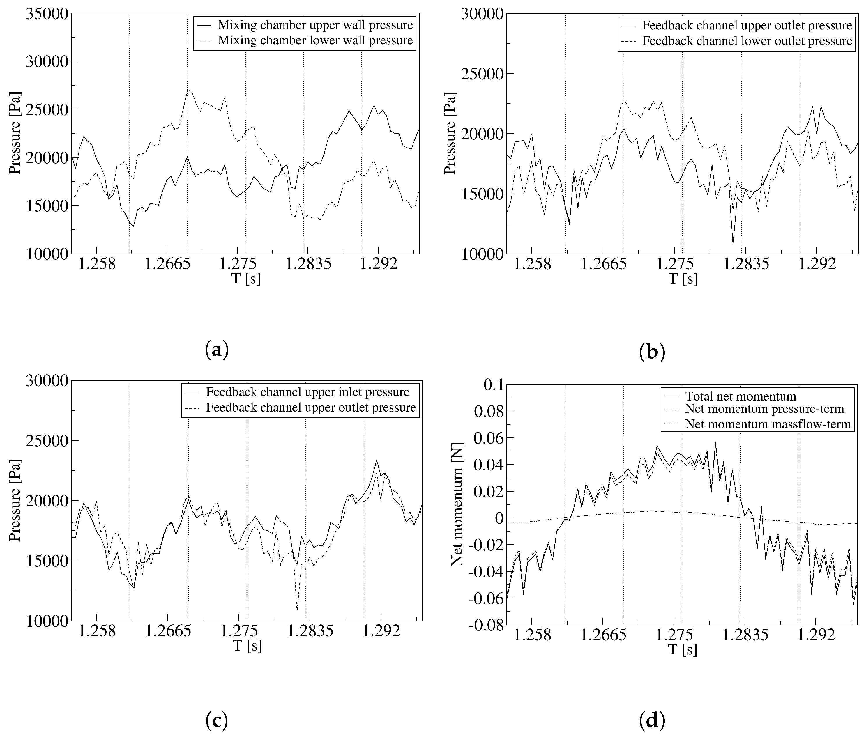
The initial time in Figure 4, T = 0, was chosen at the instant at which the volumetric flow across the FO upper outlet was minimum. At this particular instant there is some negative flow entering the oscillator across the oscillator upper outlet, see Figure 5a at a dimensional time of 1.255 s. The jet inside the MC is moving down and it is about to reach its lowest position, Figure 5c clarifies this point. According to Figure 4a, there is a considerable flow along the upper feedback channel, from Figure 5b it is observed that such volumetric flow is almost at its maximum value and it tends to decrease over time. When comparing Figure 5a,b, it is stated that the FC volumetric flow is one order of magnitude smaller than the oscillator volumetric flow. This characteristic agrees perfectly well with what was found in [13,19] working with air, comparing Figure 5a,b from the present paper with Figures 6 and 8 in [19] or with Figures 3 and 5 from [13]. At this initial instant, the volumetric flow along the lowest FC is almost zero, see Figure 5b. The spatially averaged pressure at the MC upper converging surface is about 4000 Pa higher than the one corresponding to the lower converging wall, this can be seen in Figure 4d and Figure 6a, and both pressures are about to decrease versus time. Also, the pressure at the upper FC outlet, see Figure 6b, is about 4000 Pa higher than the one appearing at the lower FC outlet, indicating there must be a force acting on the main jet inlet which pushes the jet down. The net momentum acting onto the lateral sides of the jet at the MC inlet is obtained when considering the pressure and mass flow on both FC outlets. The pressure at each grid cell multiplied by the cell area and summed across a feedback channel outlet provides the momentum due to the pressure at this particular section. However, the momentum due to the pressure needs to be added to the momentum due to the FC mass flow, which was determined via dividing the instantaneous mass flow raised to the power of two by the section of the feedback channel outlet and the fluid density, $M=ps+\dot{m}v=ps+{\dot{m}}^2/\left(\rho s\right)$. Each separate net momentum, pressure, and mass flow term on both FC outlets, and the addition of both terms, is presented in Figure 6d, from which it is stated that the net momentum due to the mass flow is almost negligible when compared to the one generated by the pressure. The net momentum presented in Figure 6d is almost the same as the net momentum due to pressure term, then the forces due to the FC mass flow are over an order of magnitude smaller. The net momentum at this initial time is negative, indicating the jet is being pushed down, in fact the net momentum has just reached its maximum negative value. Notice there is a very good agreement between Figure 6b,d, in fact, the origin of Figure 6d is the temporal pressure difference between both feedback channel outlets.

Going back to Figure 4a, it is observed that the bubble located between the jet and the MC lower borders is about to reach its minimum volume, while the bubble above the jet is almost at its maximum dimension. Notice that these bubbles consist of a series of small vortical structures, instead of a main large structure as defined in previous papers, see for example [17,19]. This is probably due to the high accuracy of the turbulent model employed along with a very realistic three dimensional model presented in this research. When analyzing the vortical structures generated, it needs to be considered that the Reynolds number studied is relatively high, hence the flow is chaotic. Evaluating a different FO configuration and using the Q criterion, the internal vortical structures were presented in [32].

At this initial instant, the jet leaves the FO through the lower outlet. On both sides of the (EC), a large vortex is observed, the lower vortex is smaller than the upper one and has a much higher intensity, see from Figure 4d that the pressure is about 32% smaller than the upper one, indicating that the lower vortex turns much faster. The pressure inside the mixing chamber is quite homogeneous, and some particular low pressure spots are to be seen where the main lower and upper bubbles are located. The particularly low pressure spot located below the jet indicates the Coanda effect appears in this location. According to [41], from this low pressure location and when the flow is considered as compressible, weak expansion waves are being generated.

At this initial instant, on the MC upper converging surface, the pressure is about 16% higher than the one existing on the MC lower converging surface. This particularly high stagnation pressure point will move to the lower converging surface in the next time period T = 1/6, compare Figure 4d,e. It appears the jet impinges alternatively on these surfaces during a small period of time. According to Gregory and Tomac [41], under compressible flow conditions, weak compression pressure waves are generated alternatively at these locations. The FC upper branch has a slightly higher pressure than the lower branch, see Figure 4d, and this pressure difference between both feedback channels and measured at the feedback channels outlets is presented in Figure 6b. The particular pressure difference between the upper feedback channel inlet and outlet is introduced in Figure 6c. The pressure is very much alike along the channel, being just slightly higher at the inlet, but this small pressure difference is what drives the flow along the feedback channel. It is at this point relevant to clarify that all graphs presented, especially the pressure ones, show very scattered curves. The origin of this lack of smoothness is the intrinsic instabilities associated with the chaotic flow. Another point to discuss is that the curves presented are not fully sinusoidal. As the flow inside the mixing chamber is fully turbulent, the jet inside the mixing chamber does not follow a perfect and symmetrical displacement, therefore the periods of all variables are not completely sinusoidal.

In the next time period T = 1/6, the jet inside the MC has reached its lowest position and it is starting to move up. Most of the flow is leaving the oscillator through the lower oscillator outlet, but some amount of flow exits the oscillator through the upper outlet, see Figure 4b and Figure 5a. Two large vortices can be observed at the external chamber upper and lower outlets. The vortex associated with the upper outlet is much bigger than the one appearing at the lower outlet, yet the intensity associated with the lower vortex is higher, as can be extracted from the observation of the pressure field in Figure 4e. In any case, when comparing Figure 4d,e it is observed that the external chamber lower vortex has decreased its intensity versus the previous time period, which is because the mass flow leaving through the lower outlet is now smaller than the previous time period. The volumetric flow along both feedback channels is very similar and flows in both cases from the feedback channels inlets to the outlets. This fact can be observed from the streamlines plot presented in Figure 4b and from the FC volumetric flow at a dimensional time of 1.2635 s, Figure 5b. The maximum pressure is now to be observed at the MC lower converging wall, see Figure 4e and Figure 6a, which is why the lower FC has a slightly higher pressure than the upper one, yet as already mentioned, the volumetric flow is almost the same in both feedback channels, which seems to indicate that there is a phase lag between the instant an FC is pressurized and the instant the flow starts moving along the FC. In fact, at this particular instant and according to Figure 6b, the pressure on both feedback channel outlets is almost the same, although on the verge of being higher at the lower FC outlet. From the information presented in Figure 6b, the pressure term of the net momentum applied to the jet entering the FO is obtained, see Figure 6d, where it can be stated that at this instant, the net momentum is almost zero. Figure 5c,d presents the jet inclination angle at the mixing chamber inlet and outlet, as already introduced by Seo et al. [22]. The jet inclination angle at the MC inlet is still negative and tending to zero, while at the MC outlet the jet inclination angle is now positive, see Figure 4b and Figure 5d. It is interesting to realize that at this instant the jet leaving the MC is facing upwards, but the jet still leaves the oscillator through the lower outlet, which is due to the reattachment the jet is having to the external chamber lower wedge surface.

When moving to the next time period, T = 1/3, it is observed that the jet is now entering the MC almost perpendicular to it, see Figure 4c and also Figure 5c, where it can be stated that the jet inclination angle at the mixing chamber inlet is slightly positive. The flow is leaving the oscillator through the upper outlet, see Figure 4c and Figure 5a. This is why at the MC outlet, the jet inclination angle is positive and having almost its maximum value, Figure 5d. The two typical vortices respectively appearing at each side of the external chamber are clearly seen, at this particular instant. The lower vortex, which is located at the center of the lower outlet, has a slightly higher intensity than the upper one, see Figure 4f. This is particularly relevant because at this instant the jet leaves the actuator through the upper outlet, which in reality indicates that the jet has just flipped from the lower outlet to the upper one. Inside the MC, the maximum pressure is localized at the lower converging surface, notice that the jet impinges on this surface, Figure 4f. As a result of the location of the maximum stagnation pressure point, the lower feedback channel is pressurized and a large amount of flow is going from the feedback channel inlet to the outlet, with Figure 4c,f and Figure 5b are showing this situation. Despite the fact that the flow on the lower FC is almost at its maximum, on the upper FC there is still a small amount of flow from the FC inlet to the outlet. Regarding the streamlines at the lower FC, it is interesting to recall the work undertaken by Woszidlo et al. [19], where they defined the existence of a bubble at the FC inlet, which perfectly fits with what can be seen in Figure 4c. At this particular instant, the pressure between the lower and upper mixing chamber converging walls is about 6500 Pa, also the pressure difference between the feedback channel lower and upper outlets reached a particularly high value of about 3000 Pa, see Figure 6a,b. As a result of the relevant pressure difference at the feedback channel outlets, the positive net momentum acting on the jet is about to reach its maximum value, see Figure 6d.

The next time period corresponds to T = 1/2, see Figure 4g,j. The jet inside the MC is about to reach its maximum position, the flow is leaving the actuator through the upper outlet, and the jet inside the MC is still impinging onto the lower converging surface. The stagnation pressure is lower than the one existing in the previous time period. The pressure on the lower converging wall, see Figure 4j and Figure 6a, is much higher than the one in the upper converging wall. The lower FC is still pressurized, and the flow rate going from the lower FC inlet to the outlet is still very high, on the other hand the flow flowing along the upper FC is almost zero, see Figure 4g and Figure 5b. The pressure on the lower FC outlet is, according to Figure 6b, about 4000 Pa higher than the one on the upper FC outlet. This is why the net momentum acting on the jet inlet is positive, pushing the jet upwards, Figure 6d represents this case.

At T = 2/3, Figure 4h,k, the jet at the MC has reached its highest position and is beginning to move down. At the MC inlet, the jet inclination angle is still positive, but tending to zero, see Figure 5c. At the MC outlet, the jet inclination angle has changed from positive to negative, see Figure 4h and Figure 5d, but the jet still leaves the FO through the upper outlet, the volumetric flow through the FO upper outlet is represented in Figure 5a. The vortex generated at the upper part of the external chamber is now more energetic than the one appearing at the lower external chamber outlet, and Figure 4h,k clarifies this point. From Figure 6a it is observed that the maximum stagnation pressure has moved to the upper converging wall, and the upper FC is about to be pressurized. The pressure at both feedback channel outlets is very much the same (Figure 6b), as a result the volumetric flow along both feedback channels is also very similar, see Figure 5b, and flows from the feedback channels inlets to outlets. The net momentum applied to the jet entering the MC, as can be observed in Figure 6d, is almost null, this is clearly understandable when realizing that the pressure on both feedback channels outlets is nearly the same, as represented in Figure 6b.

Finally, when the time period is T = 5/6, the jet is located at the center of the MC and descending down, the jet inclination angle at the MC inlet is slightly negative and so is the jet at the MC outlet, see Figure 4i and Figure 5c,d. The flow is leaving the FO through the lower outlet, in fact, there is some reverse flow entering the FO through the upper outlet, as presented in Figure 5a. At the external chamber upper outlet, a clear vortex is being observed, as can be seen in Figure 4l. This vortex has a higher intensity than the one appearing at the external chamber lower outlet. This is particular because, as previously mentioned, the fluid leaves the oscillator through the lower outlet, which in reality indicates that the jet at the external chamber has just flipped over from up to down. Inside the MC, the jet is still impinging on the upper converging surface, Figure 4l, as a result there is a relatively large flow moving along the upper FC. On the lower FC there is a small amount of flow still going from the FC inlet to the outlet, see Figure 5b. The pressure difference between the upper and lower converging walls is at its maximum, about 6000 Pa, and so is the pressure difference between the feedback channel upper and lower outlets, about 3000 Pa, see Figure 6a,b, respectively. As a result of the pressure difference existing between the feedback channels outlets, the net momentum acting on the lateral surfaces of the jet entering the mixing chamber is negative, see Figure 6d, and the jet is being pushed down. Two videos presenting the dynamic velocity field and the pressure distribution are given as Supplementary Materials.

Based on the previous explanations, the following statement is made: What is needed to flip the jet from one side to another is a pressure gradient between the feedback channel outlets. Once a pressure threshold is overcome, the jet starts bending and the mass flow through the feedback channels provides the required volume for the mixing chamber bubbles to expand. The required pressure threshold originates at the mixing chamber outlet converging surfaces.

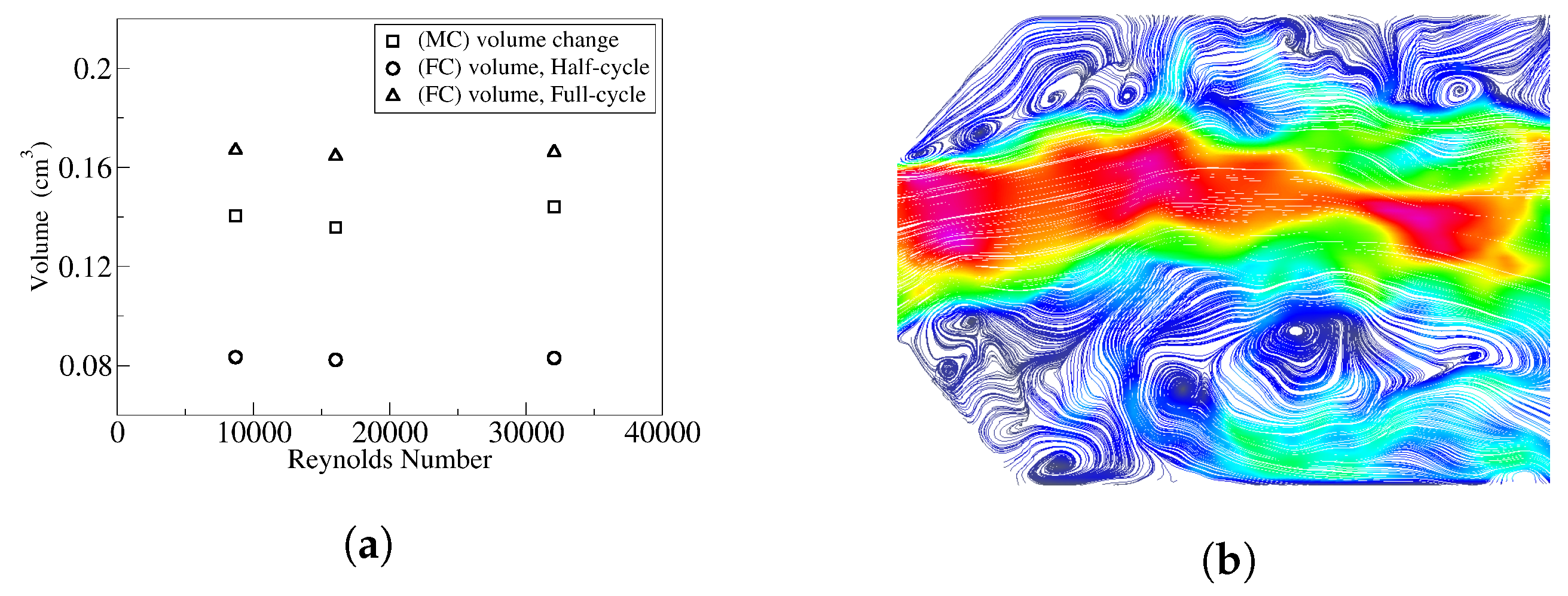
Figure 7 introduces, for the three Reynolds numbers studied, 8711, 16,034, and 32,068, the volume of fluid transferred through each FC during half cycle and during a full cycle. The estimated mixing chamber bubble volume increase, as the main jet flips from one side to the other, is also presented. According to the work undertaken by [18,19], the maximum bubble volume remains constant and independent of the Reynolds number employed, and the volume of fluid transferred by the feedback channel, according to [18,19,22], was always equal to the bubble volume growth. Figure 7a shows that both volumes are independent of the Reynolds number, yet they are not equal, which means the volume of fluid required for the mixing chamber bubble to expand may not be fully provided by one of the feedback channels flow, in fact both FCs are responsible for the MC bubble growth. It also appears that some of the required volume is provided by the mixing chamber incoming jet, and Figure 7b clarifies this point. Notice that the jet expands as it enters the MC, filling up part of it.

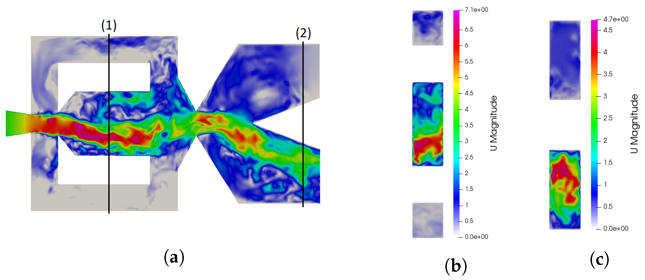
At this point, it is necessary to remember that most of the previous work on fluidic oscillators was done in 2D, and even the results obtained experimentally were based on 2D PIV measurements. The present simulations are 3D, and this fact is likely to explain the small discrepancies found regarding the origin of the fluid required for the mixing chamber bubble to grow. In order to highlight the importance of performing the study in 3D, Figure 8 introduces instantaneous slices of the mixing chamber and of the FO output exits. Clearly, the flow cannot be considered two dimensional at any point and clarifies the difficulty of measuring the exact bubble growth in the mixing chamber.

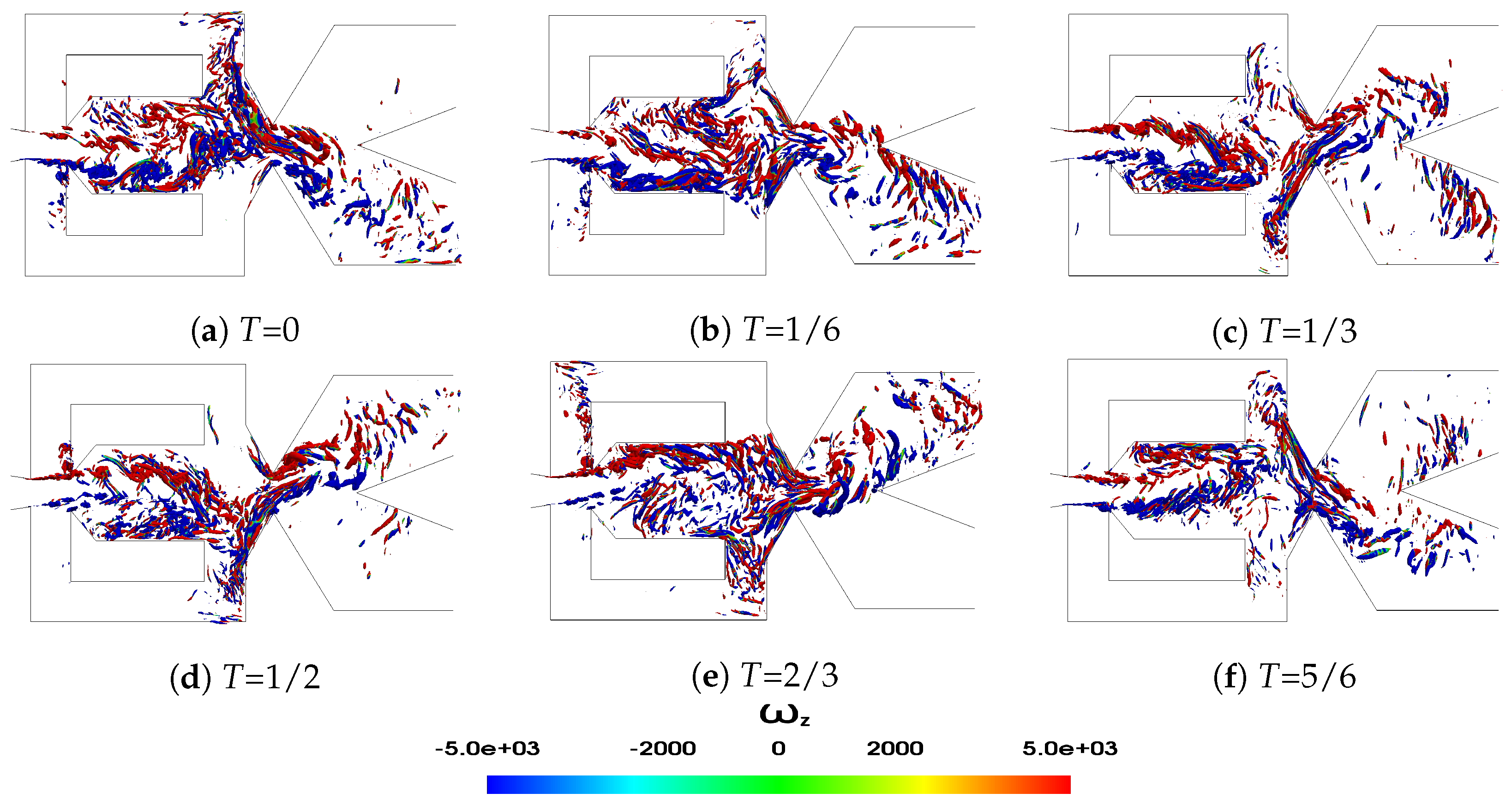
A good way to illustrate the vortical structures appearing inside the FO is by means of isosurfaces based on the Q criterion, as presented in Figure 9. The isosurfaces are colored by the vorticity about the Z axis. The color blue indicates the structures turn clockwise, the red color is associated with counterclockwise rotation. The snapshot sequence presented in Figure 9 characterizes a full oscillation period divided into six evenly spaced time steps, which match with the time steps introduced in Figure 4. It is interesting to see the coexistence of positive and negative structures at any instant. When the jet inside the MC is inclined downwards, T = 0 and T = 1/6, the negative structures dominate the flow, but the counterclockwise structures are the predominant ones when the jet inside the MC faces upwards, T = 1/2 and T = 2/3. The vortical structures inside the FCs and the external chamber (EC), which could clearly be seen in Figure 4, can hardly be seen in Figure 9, indicating that their vorticity is at least an order of magnitude smaller than the one associated with the MC vortical structures. The large coherent negative structures which can be seen in Figure 9a,b break and move downstream of the MC at time T = 1/3. In the next two time periods, in Figure 9d,e, coherent positive structures dominate the MC flow, also moving downstream, while breaking up on the next time step.

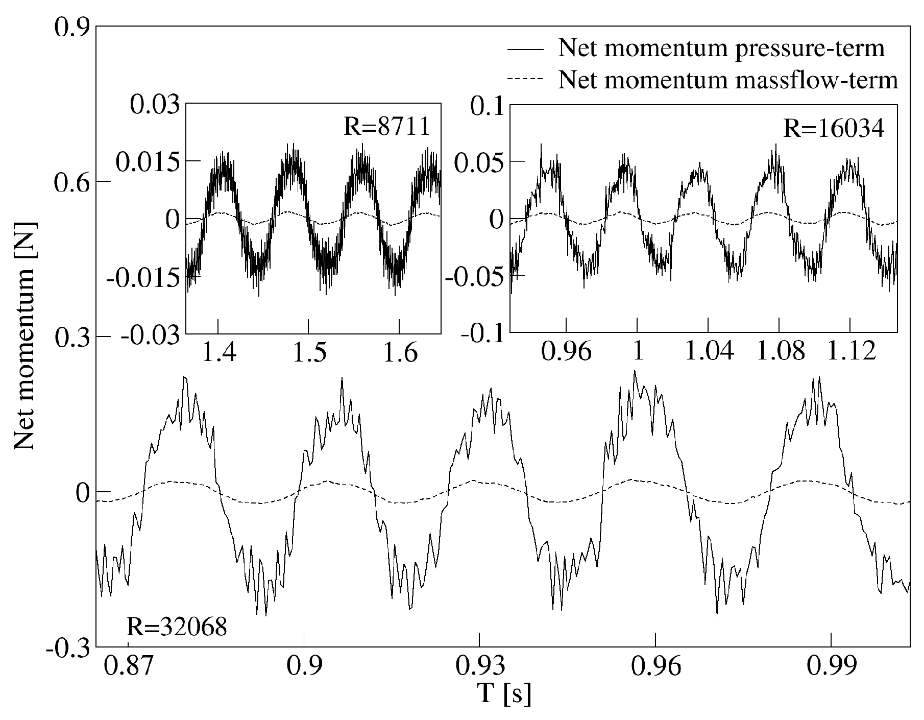
4.2. Variation of the Fluidic Oscillator Momentum with the Reynolds Number

When evaluating the forces which trigger the flapping motion of the incoming jet inside the mixing chamber, and according to previous studies, it seemed that the mass flow flowing along the feedback channels had a high degree of relevance. In the previous section, see Figure 6d, the net momentum generated by the FC mass flow was compared with the one generated by the pressure, and both net momentums were determined at the feedback channels outlets. The conclusion was that the net momentum due to pressure is the relevant one. But one question still remains: Is the net momentum due to the pressure always the relevant one? In the present section and for three different Reynolds numbers, 8711, 16,034, and 32,068, the net momentum acting on the fluidic oscillator incoming jet and due to the feedback channels flow is compared with the net momentum generated by the static pressure. Figure 10 presents, for the three Reynolds numbers evaluated, both net momentums acting on the MC incoming jet lateral sides. The net momentum due to the static pressure and regardless of the Reynolds number studied is over one order of magnitude higher than the one generated by the feedback channel mass flow. The overall net momentum is mostly due to the pressure term, as shown in Figure 6d for Reynolds number 16,034. The conclusion is, that for the present FO configuration, the mass flow transported by the FCs plays a negligible role when considering the flapping movement of the jet inside the MC. The flapping movement is driven by the pressure difference acting onto the main jet lateral surfaces, the feedback channel output surfaces.

From Figure 10 it is also observed that the net momentum due to the pressure field appears to be rather scattered. The curve is not smooth, and the authors believe this is due to the turbulence intensity associated with the chaotic flow. Another point to be highlighted from Figure 10 is that the amplitude of the net momentum due to the pressure term increases as the Reynolds number increases. To understand why this is so, it just needs to be remembered that the kinetic energy $V^2/2$, and therefore the dynamic term of the stagnation pressure $P_{0d}=\rho V^2/2$, increases with the fluid velocity to the power of two. The peak to peak amplitude of the stagnation pressure, measured in Pascals, at the mixing chamber converging walls and as a function of the Reynolds number, was found to be having the following relation, $P{A}_{peaktopeak}=6.476\times {10}^{(-5)}\times {\left(Re\right)}^{1.985}$. The reason why it is not increasing as a function of the velocity to the power two is due to the inclination of the MC converging walls where the jet impinges.

For the Reynolds numbers studied, the net momentum peak to peak amplitude, given in Newtons, increases with the Reynolds number increase and obeys to the following expression, $M{A}_{peaktopeak}=6.267\times {10}^{(-10)}\times {\left(Re\right)}^{1.981}$. At this point, it is important to recall that the fluid net momentum has two terms, the static pressure term and the mass flow one, the second being much smaller than the first. The fluid velocity increases linearly with the Reynolds number increase, the net momentum amplitude increases with the stagnation pressure increase at the MC converging walls, and the stagnation pressure increase is a function of the square of the fluid velocity, $P_{0d}=\rho V^2/2$. Therefore, it seems the net momentum amplitude should increase as a function of the Reynolds number to the power of two, yet this is not happening and the reason why is related to the stagnation pressure increase, which in reality increases to the power of 1.985 as presented in the previous paragraph. The reason why the momentum increases to the power 1.981 instead of 1.985, which is the power increase of the pressure amplitude, is due to the pressure losses existing between the MC outlet inclined walls and the FC outlet. In reality, the fluidic oscillator internal configuration, and especially the angle of the MC converging walls, play a decisive role in the relation fluid velocity and stagnation pressure.

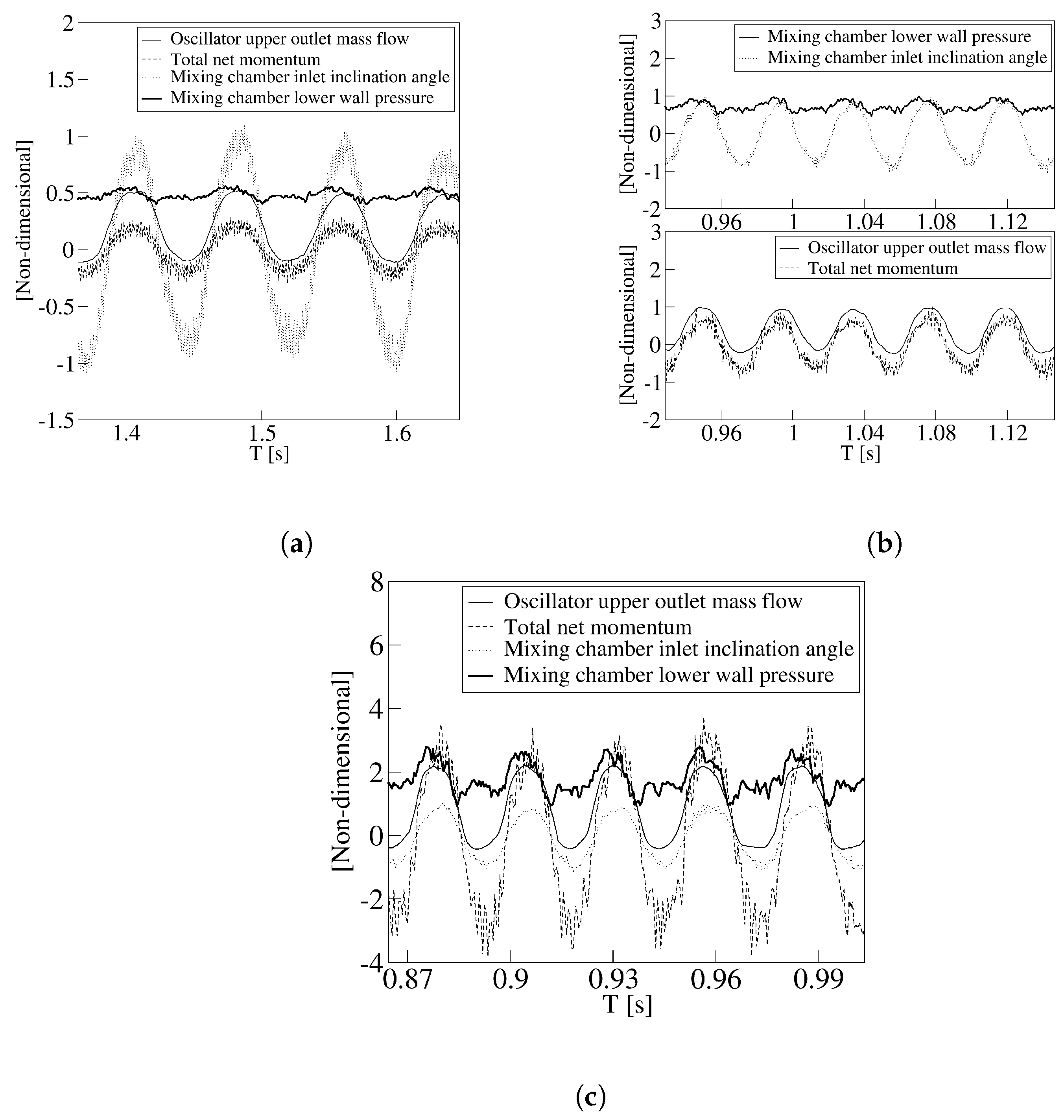
The statements made in the previous section were: the oscillation of the FO is triggered by the pressure difference between the FC outlets, and this pressure difference is generated at the MC outlet converging surfaces. In order to properly understand these statements, the following dynamic non-dimensional parameters were compared in Figure 11: the stagnation pressure at the MC lower converging surface, the net momentum acting on the jet, the MC incoming jet oscillation angle, and the FO upper outlet mass flow. These parameters were compared for the three Reynolds numbers studied, 8711, 16,034, and 32,068.

The first thing to realize, when comparing the Figure 11a–c, is that the outlet mass flow frequency and peak to peak amplitude increase as the Reynolds number increases. During approximately one fourth of the period the volumetric flow at the FO outlet enters the oscillator, the volumetric flow entering the oscillator increases as the Reynolds number increases, yet the time at which this is happening keeps being approximately one fourth of the oscillation period. The main conclusion from Figure 11a–c is that there is a perfect agreement between the dynamic parameters evaluated. This agreement exists regardless of the Reynolds number studied. The stagnation pressure peak to peak amplitude increases as the Reynolds number increases, and the exact dimensional relation previously defined was $P{A}_{peaktopeak}=6.476\times {10}^{(-5)}\times {\left(Re\right)}^{1.985}$. The net momentum applied to the jet, the FO output mass flow, and the MC inlet inclination angle follow the pressure dynamics generated at the MC outlet converging walls. Yet a small phase-lag between the stagnation pressure fluctuation and the net momentum acting on the MC incoming jet, to the order of 0.0017 s, is to be observed at Reynolds number 16,034, the phase-lag increases to 0.00287 s for a Reynolds number of 32,068.

Under compressible flow conditions, the time required by the pressure waves to travel from the FC inlet to outlet directly depends on the speed of the pressure waves, which is defined as $C=\sqrt{\beta /\rho }$, and considering the bulk modulus and the density for the working fluid, water, the resultant speed is of $C=1460$ m/s. This speed is meant to be infinite when the fluid is considered incompressible. In any case and considering the actual FC length, the phase lag between all parameters studied has to be negligible regardless of the Reynolds number employed. Therefore, the phase lag observed in Figure 11 is believed to estimate the time required for the pressure to be established at the FC outlets. In Figure 7, it was shown that the maximum volume between the MC oscillating jet and the lateral walls remained constant and independent of the Reynolds number. Figure 11 also presents the jet inclination angle at the MC inlet. Notice that the maximum inlet inclination angle remains constant and independent of the Reynolds number, therefore explaining why the maximum volume at the MC remains constant.

5. Conclusions

A careful 3D-CFD evaluation of a fluidic oscillator under turbulent conditions has been performed. Numerical results obtained were compared with previous experimental works, showing good agreement. For the Reynolds numbers studied, the flow is chaotic, therefore three dimensional simulations are needed to properly characterize the flow structures. The main jet oscillation at the mixing chamber inlet and outlet has been linked with the feedback channels mass flow, the oscillator mass flow, the pressure at the mixing chamber converging walls, and the pressure at the feedback channels outlet. The conclusion is that the forces acting onto the incoming jet at the mixing chamber inlet and feedback channel outlets are mostly due to the static pressure.

The net momentum pressure term acting onto the lateral sides of the mixing chamber incoming jet directs the oscillation of the jet in the MC, and therefore the oscillation at the fluidic oscillator output. For the actual FO, the momentum oscillation is generated by the stagnation pressure oscillation occurring at the mixing chamber outlet converging surfaces. The momentum due to the mass flow flowing along the feedback channels plays a negligible role, when considering the forces driving the oscillation. The amplitude of the net momentum oscillation is directly linked with the maximum and minimum values of the stagnation pressure appearing at the mixing chamber outlet converging surfaces, and the amplitude of the stagnation pressure increases the Reynolds number increases, according to the function $P{A}_{peaktopeak}=6.476\times {10}^{(-5)}\times {\left(Re\right)}^{1.985}$. Regardless of the Reynolds number employed, the total dynamic momentum acting on the jet always follows the stagnation pressure dynamics observed at the mixing chamber converging walls, therefore indicating that the origin of the fluctuations is the same for all Reynolds numbers studied.

References

1. Cattafesta, L.N., III; Sheplak, M. Actuators for active flow control. Annu. Rev. Fluid Mech. 2011, 43, 247–272. [Google Scholar] [CrossRef] [Green Version]
2. Corke, T.C.; Enloe, C.L.; Wilkinson, S.P. Dielectric barrier discharge plasma actuators for flow control. Annu. Rev. Fluid Mech. 2010, 42, 505–529. [Google Scholar] [CrossRef]
3. Guyot, D.; Bobusch, B.; Paschereit, C.O.; Raghu, S. Active combustion control using a fluidic oscillator for asymmetric fuel flow modulation. In Proceedings of the 44th AIAA/ASME/SAE/ASEE Joint Propulsion Conference & Exhibit, Hartford, CT, USA, 21–23 July 2008; p. 4956. [Google Scholar]
4. Raman, G.; Packiarajan, S.; Papadopoulos, G.; Weissman, C.; Raghu, S. Jet thrust vectoring using a miniature fluidic oscillator. Aeronaut. J. 2005, 109, 129–138. [Google Scholar] [CrossRef] [Green Version]
5. Seele, R.; Tewes, P.; Woszidlo, R.; McVeigh, M.A.; Lucas, N.J.; Wygnanski, I.J. Discrete sweeping jets as tools for improving the performance of the V-22. J. Aircr. 2009, 46, 2098–2106. [Google Scholar] [CrossRef]
6. Cerretelli, C.; Kirtley, K. Boundary layer separation control with fluidic oscillators. J. Turbomach. 2009, 131, 041001. [Google Scholar] [CrossRef]
7. Culley, D.E.; Bright, M.M.; Prahst, P.S.; Strazisar, A.J. Active flow separation control of a stator vane using embedded injection in a multistage compressor experiment. J. Turbomach. 2004, 126, 24–34. [Google Scholar] [CrossRef]
8. Hossain, M.A.; Prenter, R.; Lundgreen, R.K.; Ameri, A.; Gregory, J.W.; Bons, J.P. Experimental and numerical investigation of sweeping jet film cooling. J. Turbomach. 2018, 140, 031009. [Google Scholar] [CrossRef] [Green Version]
9. Seifert, A.; Stalnov, O.; Sperber, D.; Arwatz, G.; Palei, V.; David, S.; Dayan, I.; Fono, I. Large trucks drag reduction using active flow control. In The Aerodynamics of Heavy Vehicles II: Trucks, Buses, and Trains; Springer: Berlin/Heidelberg, Gemany, 2009; pp. 115–133. [Google Scholar]
10. Raman, G.; Raghu, S. Cavity resonance suppression using miniature fluidic oscillators. AIAA J. 2004, 42, 2608–2612. [Google Scholar] [CrossRef]
11. Uzol, O.; Camci, C. Experimental and computational visualization and frequency measurements of the jet oscillation inside a fluidic oscillator. J. Vis. 2002, 5, 263–272. [Google Scholar] [CrossRef]
12. Huang, R.F.; Chang, K.T. Fluidic oscillation influences on v-shaped bluffbody flow. AIAA J. 2005, 43, 2319–2328. [Google Scholar] [CrossRef]
13. Ostermann, F.; Woszidlo, R.; Nayeri, C.; Paschereit, C.O. Experimental comparison between the flow field of two common fluidic oscillator designs. In Proceedings of the 53rd AIAA Aerospace Sciences Meeting, Kissimmee, FL, USA, 5–9 January 2015; p. 0781. [Google Scholar]
14. Gokoglu, S.; Kuczmarski, M.; Culley, D.; Raghu, S. Numerical studies of a supersonic fluidic diverter actuator for flow control. In Proceedings of the 5th Flow Control Conference, Chicago, IL, USA, 28 June–1 July 2010; p. 4415. [Google Scholar]
15. Gokoglu, S.; Kuczmarski, M.; Culley, D.; Raghu, S. Numerical studies of an array of fluidic diverter actuators for flow control. In Proceedings of the 41st AIAA Fluid Dynamics Conference and Exhibit, Honolulu, HI, USA, 27–30 June 2011; p. 3100. [Google Scholar]
16. Krüger, O.; Bobusch, B.C.; Woszidlo, R.; Paschereit, C.O. Numerical Modeling and Validation of the Flow in a Fluidic Oscillator. In Proceedings of the 21st AIAA Computational Fluid Dynamics Conference, San Diego, CA, USA, 24–27 June 2013; p. 3087. [Google Scholar]
17. Bobusch, B.C.; Woszidlo, R.; Bergada, J.; Nayeri, C.N.; Paschereit, C.O. Experimental study of the internal flow structures inside a fluidic oscillator. Exp. Fluids 2013, 54, 1559. [Google Scholar] [CrossRef]
18. Gaertlein, S.; Woszidlo, R.; Ostermann, F.; Nayeri, C.; Paschereit, C.O. The time-resolved internal and external flow field properties of a fluidic oscillator. In Proceedings of the 52nd Aerospace Sciences Meeting, National Harbor, MD, USA, 13–17 January 2014; p. 1143. [Google Scholar]
19. Woszidlo, R.; Ostermann, F.; Nayeri, C.; Paschereit, C. The time-resolved natural flow field of a fluidic oscillator. Exp. Fluids 2015, 56, 125. [Google Scholar] [CrossRef] [Green Version]
20. von Gosen, F.; Ostermann, F.; Woszidlo, R.; Nayeri, C.; Paschereit, C.O. Experimental investigation of compressibility effects in a fluidic oscillator. In Proceedings of the 53rd AIAA Aerospace Sciences Meeting, Kissimmee, FL, USA, 5–9 January 2015; p. 0782. [Google Scholar]
21. Pandey, R.J.; Kim, K.Y. Numerical modeling of internal flow in a fluidic oscillator. J. Mech. Sci. Technol. 2018, 32, 1041–1048. [Google Scholar] [CrossRef]
22. Seo, J.; Zhu, C.; Mittal, R. Flow Physics and Frequency Scaling of Sweeping Jet Fluidic Oscillators. AIAA J. 2018, 56, 1–12. [Google Scholar] [CrossRef]
23. Wu, Y.; Yu, S.; Zuo, L. Large eddy simulation analysis of the heat transfer enhancement using self-oscillating fluidic oscillators. Int. J. Heat Mass Transf. 2019, 131, 463–471. [Google Scholar] [CrossRef]
24. Kara, K. Numerical study of internal flow structures in a sweeping jet actuator. In Proceedings of the 33rd AIAA Applied Aerodynamics Conference, Dallas, TX, USA, 22–26 June 2015; p. 2424. [Google Scholar]
25. Metka, M.; Gregory, J.; Sassoon, A.; McKillen, J. Scaling considerations for fluidic oscillator flow control on the square-back Ahmed vehicle model. SAE Int. J. Passeng. Cars-Mech. Syst. 2015, 8, 328–337. [Google Scholar] [CrossRef]
26. Shmilovich, A.; Yadlin, Y.; Whalen, E.A. Numerical Simulations of an Airplane with an Active Flow Control System. In Proceedings of the 8th AIAA Flow Control Conference, Atlanta, GA, USA, 25–29 June 2018; p. 3929. [Google Scholar]
27. Slupski, B.Z.; Kara, K. Effects of Geometric Parameters on Performance of Sweeping Jet Actuator. In Proceedings of the 34th AIAA Applied Aerodynamics Conference, Washington, DC, USA, 13–17 June 2016; p. 3263. [Google Scholar]
28. Aram, S.; Lee, Y.T.; Shan, H.; Vargas, A. Computational Fluid Dynamic Analysis of Fluidic Actuator for Active Flow Control Applications. AIAA J. 2017, 56, 1–10. [Google Scholar] [CrossRef]
29. Ostermann, F.; Woszidlo, R.; Nayeri, C.N.; Paschereit, C.O. Properties of a sweeping jet emitted from a fluidic oscillator. J. Fluid Mech. 2018, 857, 216–238. [Google Scholar] [CrossRef] [Green Version]
30. Woszidlo, R.; Ostermann, F.; Schmidt, H.J. Fundamental properties of fluidic oscillators for flow control applications. AIAA J. 2019, 57, 978–992. [Google Scholar] [CrossRef]
31. Ostermann, F.; Woszidlo, R.; Nayeri, C.N.; Paschereit, C.O. The interaction between a spatially oscillating jet emitted by a fluidic oscillator and a cross-flow. J. Fluid Mech. 2019, 863, 215–241. [Google Scholar] [CrossRef] [Green Version]
32. Tomac, M.N.; Sundström, E. Adjustable Frequency Fluidic Oscillator with Supermode Frequency. AIAA J. 2019, 57, 1–11. [Google Scholar] [CrossRef]
33. Tomac, M.N.; Gregory, J.W. Phase-synchronized fluidic oscillator pair. AIAA J. 2018, 57, 670–681. [Google Scholar] [CrossRef]
34. Vatsa, V.; Koklu, M.; Wygnanski, I. Numerical simulation of fluidic actuators for flow control applications. In Proceedings of the 6th AIAA Flow Control Conference, New Orleans, LA, USA, 25–28 June 2012; p. 3239. [Google Scholar]
35. Wang, S.; Baldas, L.; Colin, S.; Orieux, S.; Kourta, A.; Mazellier, N. Experimental and numerical study of the frequency response of a fluidic oscillator for active flow control. In Proceedings of the 8th AIAA Flow Control Conference, Washington, DC, USA, 13–17 June 2016; p. 4234. [Google Scholar]
36. Bobusch, B.C.; Woszidlo, R.; Krüger, O.; Paschereit, C.O. Numerical Investigations on Geometric Parameters Affecting the Oscillation Properties of a Fluidic Oscillator. In Proceedings of the 21st AIAA Computational Fluid Dynamics Conference, San Diego, CA, USA, 24–27 June 2013; p. 2709. [Google Scholar]
37. Hirsch, D.; Gharib, M. Schlieren Visualization and Analysis of Sweeping Jet Actuator Dynamics. AIAA J. 2018, 56, 2947–2960. [Google Scholar] [CrossRef]
38. Staats, M.; Löffler, S.; Ebert, C.; Grund, T.; Weiss, J. A Fluidic Device for Active Flow Control: Simulation vs. Experiment with Emphasis on Application. In Proceedings of the 2018 Applied Aerodynamics Conference, Atlanta, GA, USA, 25–29 June 2018; p. 3336. [Google Scholar]
39. Tesař, V. Pressure-Driven Microfluidics; Artech House: Boston, MA, USA; London, UK, 2007. [Google Scholar]
40. Tesař, V. Taxonomic trees of fluidic oscillators. EPJ Web Conf. EDP Sci. 2017, 143, 02128. [Google Scholar] [CrossRef] [Green Version]
41. Gregory, J.; Tomac, M.N. A review of fluidic oscillator development. In Proceedings of the 43rd AIAA Fluid Dynamics Conference, San Diego, CA, USA, 24–27 June 2013; p. 2474. [Google Scholar]
Figure 1. Fluidic oscillator general view and its different parts, (a) original fluidic oscillator, (b) fluidic oscillator with buffer zone, (c) fluidic oscillator main parts. Flattered pipe, 1; mixing chamber (MC), 2; feedback channels (FC), 3; external chamber (EC), 4; buffer zone (BZ), 5.
Energies 12 04720 g001
Figure 2. Grid used in the present study, (a) plane view, (b) zoom view, (c) side view of the mesh at the center of the mixing chamber, see the vertical line.
Energies 12 04720 g002
Figure 3. (a) Comparison of experimental and computational fluid dynamics (CFD) results, (b) FFT of the different Reynolds numbers studied.
Energies 12 04720 g003
Figure 4. Mixing chamber period of oscillation divided in six equally spaced times, Reynolds number 16,034. Figures (ac,gi), present the streamlines plots, figures (df,jl), introduce the pressure contours.
Energies 12 04720 g004
Figure 5. Mass flow through the oscillator upper and lower outlets, (a); mass flow through the feedback channels, (b); mixing chamber inlet jet inclination angle, (c); and mixing chamber outlet jet inclination angle, (d). Reynolds number 16,034.
Energies 12 04720 g005
Figure 6. Mixing chamber outlet converging walls pressure, (a); pressure at both feedback channels outlets, (b); and pressure at the feedback channel inlet and outlet, (c). Overall momentum at the feedback channels outlet, which is acting on the jet entering the mixing chamber. The momentum is split in the component due to the mass flow flowing along the feedback channels and due to the pressure acting onto the feedback channels outlet, (d). Reynolds number 16,034.
Energies 12 04720 g006
Figure 7. (a) Mixing chamber volume growth at three different Reynolds numbers, 8711, 16,034, and 32,068. Comparison with the fluid volume provided by the FC. (b) Zoomed view of the mixing chamber inlet, where it is seen that part of the incoming fluid helps the mixing chamber bubble to grow.
Energies 12 04720 g007
Figure 8. Instantaneous velocity fields at the, (a) mixing chamber, (b) spanwise section, slice (1), (c) spanwise section at the fluidic oscillator outlet, slice (2). Reynolds number 16,034.
Energies 12 04720 g008
Figure 9. Q criterion at the mixing chamber period of oscillation divided into six equally spaced times, Reynolds number 16,034.
Energies 12 04720 g009
Figure 10. Net momentum pressure and mass flow terms for different Reynolds numbers.
Energies 12 04720 g010
Figure 11. Comparison of the stagnation pressure at the mixing chamber lower converging surface, the total momentum acting on the jet, the mixing chamber inlet oscillation angle, and the oscillator output mass flow. Reynolds numbers, 8711 (a), 16,034 (b), 32,068 (c).
Energies 12 04720 g011