Power to Hydrogen Through Polygeneration Systems Based on Solid Oxide Cell Systems


Department of Mechanical Engineering, Thermal Energy Copenhagen, Technical University of Denmark, 2800 Copenhagen, Denmark
Energies 2019, 12(24), 4793; https://0-doi-org.brum.beds.ac.uk/10.3390/en12244793
Submission received: 6 November 2019
/
Revised: 28 November 2019
/
Accepted: 12 December 2019
/
Published: 16 December 2019
(This article belongs to the Special Issue Advances in Hydrogen Production and Hydrogen Separation)
Abstract
:This study presents the design and analysis of a novel plant based on reversible solid oxide cells driven by wind turbines and integrated with district heating, absorption chillers and water distillation. The main goal is produce hydrogen from excess electricity generated by the wind turbines. The proposed design recovers the waste heat to generate cooling, freshwater and heating. The different plant designs proposed here make it possible to alter the production depending on the demand. Further, the study uses solar energy to generate steam and regulate the heat production for the district heating. The study shows that the plant is able to produce hydrogen at a rate of about 2200 kg/day and the hydrogen production efficiency of the plant reaches about 39%. The total plant efficiency (energy efficiency) will be close to 47% when heat, cool and freshwater are accounted for. Neglecting the heat input through solar energy to the system, then hydrogen production efficiency will be about 74% and the total plant efficiency will be about 100%. In addition, the study analyses the plant performance versus wind velocity in terms of heating, cooling and freshwater generation.
1. Introduction
Renewable energy production technologies are going to play a significant role in the immediate future due to global warming and its significant consequences, Therefore, it is essential to find new, effective solutions that allow for the integration of sustainable energy production techniques into the current existing systems thereby decreasing the emissions. In order to use the most energy of the renewable sources, it will be essential to use such solutions with polygeneration system to maximize the energy use. Examples such polygeneration can be the production of electricity, fuel and fresh water (instead of dissipating the excess heat to the environment).
Using electrolysis technology such as solid oxide electrolyte cells (SOECs) is one way to store the excess energy from renewable sources when the production is higher than the demand. One can then use the stored fuel to generate power and produce other useful outputs such as heat, cooling and fresh water through solid oxide fuel cells (SOFCs) when the renewable source is low, like on a calm day when using wind energy or during nighttime when using sun energy. This indicates that, then one can use a reversible solid oxide cell (RSOC) to produce synthetic fuel from electricity, or to produce electricity from fuel when reversed.
Several studies on SOEC systems have been conducted; for example, [1] reviewed technological developments in hydrogen production from an SOEC system in terms of materials, cell configuration designs, electrode depolarizations and mathematical modelling. Reference [2] presented a newly designed apparatus for testing single solid oxide cells in both fuel cell and electrolysis modes, which in turn showed performance improvements when running in electrolysis mode. Reference [3] conducted energy and exergy studies of a solid oxide cell plant to evaluate system performance in terms of energy losses, exergy destruction, and hydrogen production efficiency. Reference [4] experimented on a 16 cm2 planar solid oxide cell to test it as a fuel cell and electrolyser at various pressures ranging from 0.4 bar to 10 bar and found out that the internal resistance decreases with increasing pressure. Reference [5] showed the successful reversible operation of a dual-mode cell through electrochemical tests carried out by impedance spectroscopy and thereby proving its feasibility of the concept. Reference [6] demonstrated the heat spreading capabilities and power limitations of high-temperature applications in SOEC/SOFC stacks through an experimental study.
The European Union (EU) energy policy includes EU low-carbon roadmap milestone, which indicates a 40% reduction in carbon emissions and 30% EU-wide share of renewables. The increased renewable energy sources penetration and their irregular energy production have led to the emerging the need for energy storage technologies. This in turn means that EU energy market is changing towards application of Power to Gas (P2G) systems. Many studies discuss P2G systems based on water electrolysis, and this study mentions some of these studies. Reference [7] studied the techno-economics of P2G systems and concluded that these systems require subsides to overcome economic barriers. The study of [8] showed that an economic dispatch model involving wind power and a battery-energy storage system integrated with P2G helps to reduce the amount of wind power curtailment and stabilize fluctuations in the wind power output. Reference [9] performed a techno-economic analysis of eight different pathways scenarios including hydrogen via electrolysis. Reference [10] highlighted P2G processes and their products as a promising solution to the problems faced by the transport sector, while [11] discussed the role of and potential of deploying P2G applications for the generation, transmission and distribution of electricity. Reference [12] suggested that a smart energy network should also include a P2G system via e.g. water electrolysis, while [13] argued that the most economically affordable technology for hydrogen production is the electrolysis system using surplus wind energy in Ireland. Reference [14] presented a scenario for integrating P2G with a multi-source microgrid including wind energy, micro turbine, etc. Reference [15] performed a study on the techno-economic and environmental assessment of bio-methane production via biogas upgrading and P2G technology. Reference [16] uses a different approach, which is integrating gasification with P2G through water electrolysis. However, none of these studies present a detail plant balance as in the present study.
Direct contact membrane distillation (DCMD) is a thermal separation process that allows only water vapor (or other volatiles) to pass through a micro-porous hydrophobic membrane while no impurities such as salt can cross it. The reason is the driving process is created by the vapor pressure gradient (and by temperature difference) over both sides of the membrane. Reference [17] reviewed the desalination of seawater using DCMD systems, and their performance from laboratory scale to pilot projects thereby proving the feasibility of concept. Reference [18] showed by experiments that hot water at 80 °C under optimum conditions and with an optimum membrane selection can separate 99.99% of salt from the water. Desalination systems powered by waste heat are an attractive solution that can address the worldwide water-shortage problem, without contributing significant greenhouse gas emissions. Reference [19] also stated that low-temperature DCMD systems are a promising system for freshwater production. The study by [20] indicates that the experimental data agrees very well with the calculated results in terms of vapor mass flux and overall heat transfer coefficients. In addition, such a technique has a great advantage because it works at even lower temperatures, such as 40 °C, suggesting the use of lower temperature sources and thereby avoiding the latent heat of water [21].
This study presents a novel polygeneration system (power-to-gas) that uses the excess energy from the wind turbines to feed a RSOC system thereby producing fuel for later use. Further, the system design recovers the waste heat from the RSOC system to produce heating, cooling and fresh water in addition to fuel. Such a system will results in a flexible polygeneration plant driven mainly by wind energy that can regulate different output combinations of hydrogen, heat, cool and fresh water. The study first presents a complete balance of the plant and then offers alternative system designs for different demands. Further, this study analyses the performance of each design thermodynamically. To the best of the author’s knowledge, no similar studies exist in the open literature. The objective of this study is to discover alternative possible future power-to-gas technologies for integration into existing systems, which might be of interest for future power generation needs.
2. Modelling of the Main Components
2.1. RSOC Modelling
The model developed here is based on the model presented in [22] and [23], which uses a detailed electrochemical model and captures the experimental data very well. First, the study calculate the pressures at the gas outlets using a pressure drop parameter as input values through:
where and are the relative pressure drops at the anode and cathode sides, respectively. Then, one may calculate the cell voltage and the current density by using the power as input data:
where and are the number of stacks, number of cells per stack, cell voltage, single cell area and current density, respectively. The Nernst potential gives the theoretical minimum electrical work, but in reality, part of the voltage is lost irreversibly owing to polarizations such as ohmic, activation, and concentration polarizations. The cell voltage can be calculated by following equation:
where the cell voltage is calculated by adding the polarizations (activation, ohmic and concentration) to the Nernst voltage. Each polarization is then carefully modelled. The ohmic resistance remains constant by changing current density, while the variation of the other two resistances depends strongly on the current applied. For example, ohmic polarization increases proportionally with the current, while activation polarization and concentration polarization are dominant at low and high current levels, respectively [24]. Thus, the minimum electrical work needs to be applied to the electrolysis will be dependent on the Nernst potential plus the polarization losses.
The Nernst potential and the polarizations in the RSOC (activation, ohmic and concentration) are calculated as explained in [24] and [23]. The diffusion coefficient is approximated using the kinetic theory and the Chapman–Enskog theory [25]. Note that the energy applied through electrical work might not be enough to drive the system’s unspontaneous reactions. The remaining energy must then be applied by a heat source at higher temperature and/or by directly increasing the power (increasing the current through the cells), which in turn produces more heat owing to the Joule effect [26]. When the heat produced equals to the heat demand in the reaction (thermo-neutral point), then the voltage becomes:
where is the enthalpy change in the reactions, and F is the Faraday constant (96,485.34 C/mol). This study uses the molar balance of each element to determine outlet concentrations and mass flows, and uses current density to determine the quantity of reactions that take place. The molar production of H2 (or moles of H2O molecules split) depends directly on power supplied, cell area and current density, while O2 is produced according to the reaction:
The power, the voltage and the current are dependent on each other and therefore, if one of them is defined, the others can be determined. Another way of defining these parameters would be by fixing the H2 production or fixing the molar fraction at the outlet. Finally, the efficiency is defined as:
where and are the electrical power required to run the electrolyzer and the heat input required to preheat the water, while is the mass flow rate of hydrogen production and is the lower heating value of the hydrogen. This study assumes = 120,000 kJ/kg.
2.2. Direct Contact Membrane Desaliantion (DCMD) Modelling
For this component, the present study uses a hollow fibre configuration as described in [26]. The preheated seawater flows in the fibres (the feed side) of the DCMD, while cold water flows through the permeate side (located at the other side of the fibres). The design is made in such a way that both sides have a constant flow. Owing to the counter-flow configuration, the temperature difference along the fibre is almost constant and therefore it is the associated with vapour pressure differences. Thus, the pressure gradient across the membrane is the force that drives the entire process. The modelling along the fibre is performed by dividing the entire fibre into smaller segments or control volumes, and applying the balance equations (mass flow and energy) using the mean properties of each segment as well as the state of each segment (temperature, density, pressure, etc.). The reason for such discretization is to avoid the non-linear behaviour of the system which otherwise may lead to large errors in the results.
The operation range of the model for the mass flow of one unit is between 0.05–0.15 kg/s, while for higher mass flows, the model calculates the number of units needed for that mass flow. The range of operation for the feed temperature has limits, and in this study, it is set between 70 °C to 90 °C. The permeate flow is assumed to remain at a constant in-flow of 0.1 kg/s in each unit and at 25 °C at the inlet.
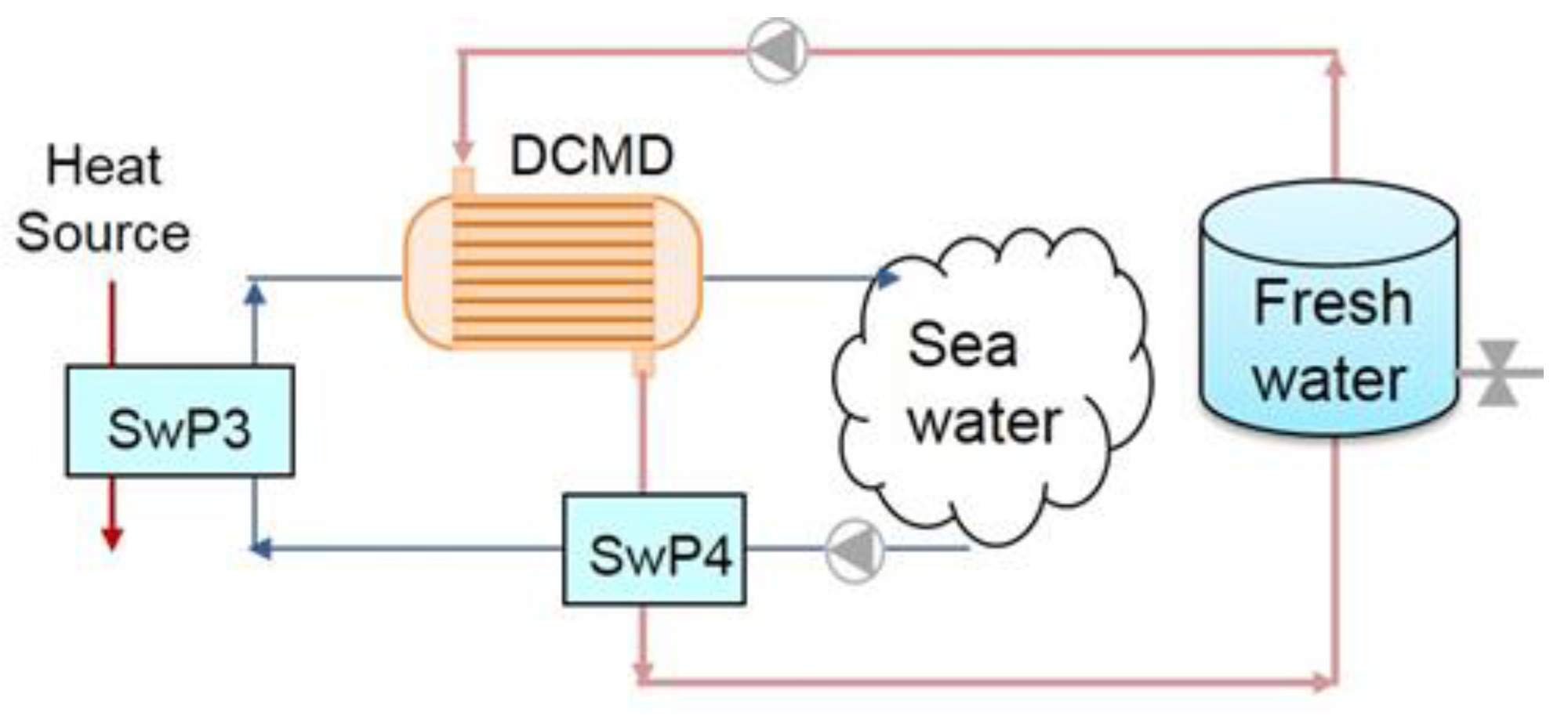
Another important issue to consider, when designing the hollow fibre operation, is the membrane liquid entry pressure, which sets the limit for the applied transmembrane pressure. Transmembrane pressure is defined as the hydrostatic pressure minus the vapour pressure ( and ). Values below such limits will prevent liquid from entering the pores. The hydrostatic pressure does not affect the permeate flux, but it is important to consider, as it prevents the pores from flooding. Figure 1 shows the DCMD plant designed in this study while Table 2 presents data related to the DCMD used here.
The design of freshwater unit is rather simple. Seawater is preheated by freshwater and by a heat source (SwP4 and SwP3 heat exchangers in the figure, respectively) before entering the DCMD. In this study, the heat source is the off-heat after the electrolyser. The freshwater loop is a closed loop and a small water pump drives it. Further, a tank collects the produced freshwater, while the non-desalinated seawater goes back to the sea again. The salt and other particles that cannot pass though the pores of the DCMD flows along with non-desalinated seawater to the sea. This study uses Reference [26] for fibre length, diameter and other parameters.
2.3. Single Stage Absorption Chiller Modelling
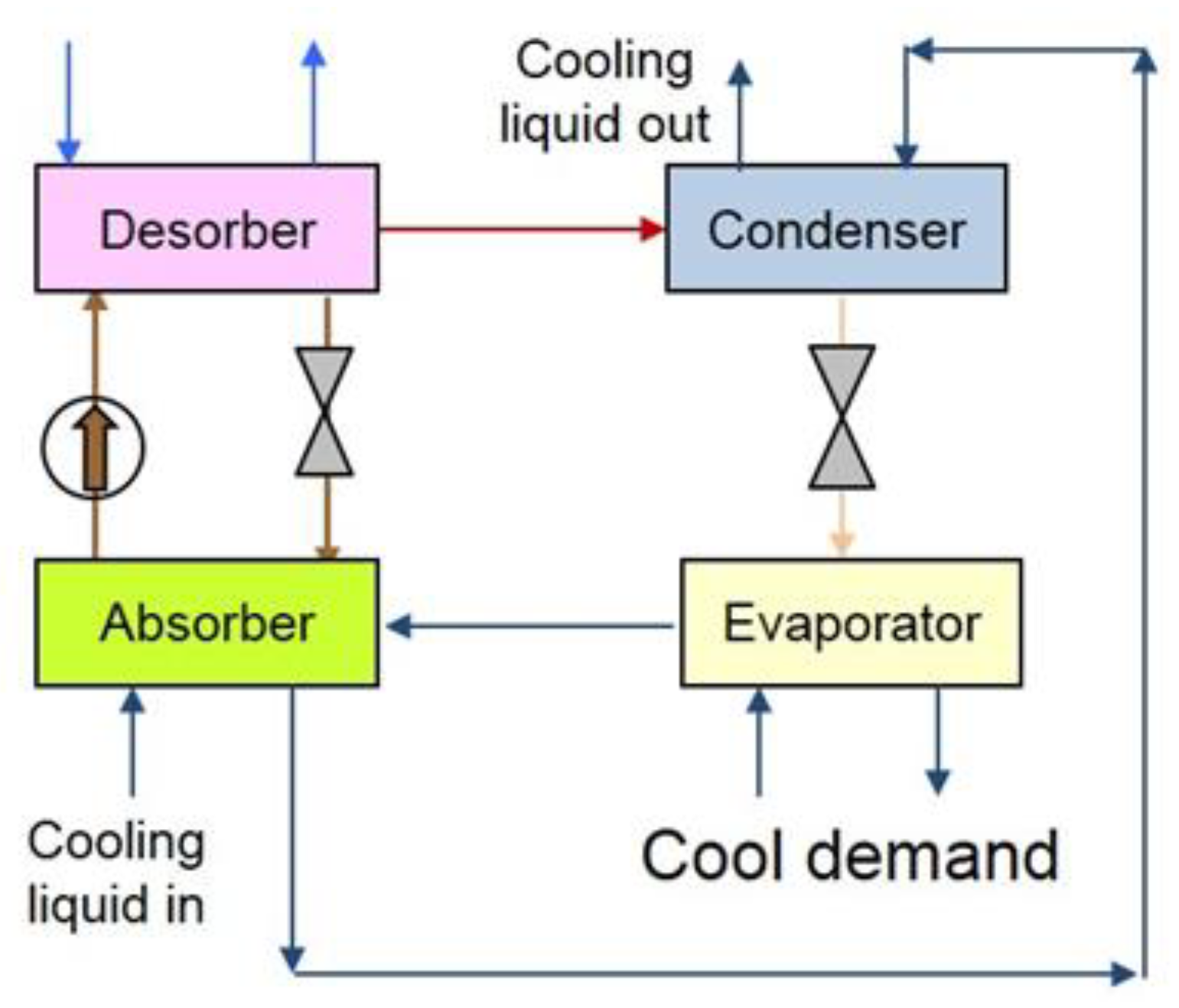
Absorption cycles are similar to vapour compression cycle, except instead of a vapour compressor (electricity driven) it uses a thermal compressor known as desorber or generator. Such thermal energy applies on a solution consisting of a refrigerant and an absorbent such as the mixture of water with lithium-bromide (LiBr) or, water with ammonia [27]. Nevertheless, their market share is still limited compared to the vapour compression systems. The fundamental reasons for this is the high initial capital costs compared to the deliver cooling. Regarding the coefficient of performance (COP), which is defined as the ratio between the achieved cooling capacity and the heat input to the cycle. Its value is usually lower than 1 (typically within 0.5 to 0.9), if the plant is a single stage. However, vapour compression cycles display values higher than 3 based on the electrical input [28] and [29]. Despite their disadvantages, the utilization of absorption cycles is significantly favoured when waste heat is available, for example waste heat from industrial processes. The integration of absorption chillers into a process with available heat leads to an increase in the overall efficiency of the plant.
The driving force of an absorption chiller cycle is a solution consisting of a refrigerant and an absorbent. In most cases, these devices utilizes a mixture of water with lithium bromide or water with ammonia. Further, the cycles can be single, double or triple effect/stage, depending on the available waste heat temperature and the potential investment. In general, multistage cycles need higher temperature heat sources. The higher the stage the higher the values for COP would be, for example double stage absorption chillers may display COP of 1.2. On the other hand, the installation is more complex since larger number of components will be required which results in higher capital costs [30]. Therefore, this study utilizes a single stage absorption chiller as displayed in Figure 2. Additionally, this study uses the mixture of water with lithium bromide (LiBr).
The desorber (generator) separates some of the refrigerant from the solution mixture, creating a weak and rich solution. Note that in the present study, the heat input to the absorption chiller is the waste heat from the RSOC plant. The weak solution routes to a condenser to lose some heat and then to a valve to lose some pressure. Now the weak solution can evaporate immediately if a proper amount of heat extracts from it. After evaporation. The weak solution, which has a very low pressure, routs to an absorber. On the other hand, the rich solution from the desorber enters a valve to lose some pressure and then enters the absorber. The absorber creates a low-pressure area that sucks the rich solution into the weak solution. The diluted solution out of the absorber is then pumped to the desorber. Both the absorber and condenser reject heat to a cooling liquid such as water and therefore a cooling liquid enters to the absorber and then continuous to the condenser. The evaporator needs heat, which is taken from the cooling flow. This study assumes that the cooling flow enters the evaporator at 11 °C and leaves it at 4 °C.
2.4. Wind Turbine Modelling
Wind turbines (WT) can be divided into two different designs according to the axis of the main shaft rotation. Hence, WTs are either horizontal axis or vertical axis. Horizontal axis wind turbines are by far the most used kind and therefore this study focuses on this kind only. Further from an operational point of view, WTs can either works at constant shaft speed or at variable shaft speed. The later has a more complex and expensive design due to their need of some extra components. On the other hand, variable wind turbines can always operate at their peak efficiency for a wide range of wind velocity. The fixed speed ones, instead, are designed to operate at their optimal efficiency only for one value of wind speed, which is statically the most probable for the place of installation.
Due to Betz law the maximum theoretical efficiency of a wind turbine is equal to 16/27 ≈ 0.593. The mechanical power of a WT is calculated as:
where , , and are air density at hub height [kg/m3], the swept area (), wind speed [m/s] and the so called power coefficient. Air density at hub height is calculated as:
where = 1.225 [kg/m3] is the air density at sea level and H is the height of turbine. The swept area is [m2]. The power coefficient is a function of pitch angle θ [°] and the tip speed ratio λ [rad]. The pitch angle allows the blades rotation along their longitudinal axis. λ is defined as:
where and R are the blade angular rotation [rad/s] (rotational speed) and rotor radius [m]. The blade angular rotation is defined as:
where n is the rotor angular velocity [rpm]. The power coefficient is defined as in [32]:
where C1 = 0.5, C2 = 116, C3 = 0.4, C4 = 0, C5 = 5, C6 = 21 and β:
The electric power is then calculated as:
where is the mechanical to electrical conversion efficiency and is the number of wind turbines in the windfarm.
Electrical power from a wind turbine strongly depends on the wind velocity, rotational speed (blades rpm) and wind direction to the blades (angle of attack). The power produced by the wind turbines are AC (alternating current) while the power feed to the electrolyser is DC (direct current), therefore the design includes an AC/DC converter, which has an efficiency of 0.95%. Further, WTs can work either at constant shaft speed or at variable shaft speed. The later have a more complex design compared to the former one due to the need for additional components. However, variable shaft speed WTs can work at their peak efficiency for a wide range of wind velocities. Table 4 presents parameters assumed in this study for basic case.
2.5. Modelling of PTSC (Parabolic Trough Solar Collector)
A model for the steam generator PTSC is developed by combining the models presented in [26,33,34]. In short, the model calculates the outlet of steam state conditions from the water flow inlet and the external atmospheric conditions. The model includes calculations of heat losses and pressure drops along the pipe. Direct solar radiation, solar ray’s angle of incidence, wind velocity are the main input data for this model. Other input parameters are the ambient temperature, sky temperature, the number of rows and their length. The model includes other dimensions and optical characteristics of the unit, such as pipe aperture (w), receiver diameter (D), reflectivity and absorptance. The model equally distributes the total incoming mass flow between the numbers of rows. Then, it divides the receiver into three sections depending on the water state, first and third sections are single-phase flow (liquid and steam respectively) while the second part is two-phase flow.
The model calculates the outlet pressure by knowing the inlet pressure and pressure drop along the tubes. The pressure drops are calculated according to the single phase (heating to saturated steam and super-heating) or phase changes (evaporating) with appropriate correlations. For the single phase Darcy–Weisbach correlation is used while for the boiling section (phase changes) the Friedel correlation is used [35]. Friedel correlation takes into account the static, momentum and friction pressure drops.
Similarly the heat flux is calculated for the three sections according to:
where is the heat absorbed by the fluid in section s, is the optical efficiency, is the irradiation, Tamb is the ambient temperature, Trom,s is the mean temperature at the outer surface of the receiver in section s, and UL is the mean heat transfer coefficient for the entire PTSC. The area of the concentrator in section s is defined as aperture and similarly, the receiver area in the corresponding section is . Dro and Ls are the receiver outer diameter and section length, respectively.
The mean heat transfer coefficient for the entire PTSC is determined using the total heat loss to the surroundings by assuming a constant mean temperature of the outer surface of the receiver and a relative coefficient of the conductive losses through the compared structure. The heat losses to the surroundings takes into account the low-pressure air conductivity, the diameters of the external surface of the receiver, the inner glass cover and external glass cover, the emissivity of the receiver, the emissivity of the glass cover, the conductivity of the glass cover, and the convection coefficient of the wind. For two-phase flow, the Gungor and Winterton method [36] is used. It combines the effect of the forced convection and the nucleate boiling weighted with coefficients. Again, similar to the process of calculating the pressure drop in two-phase flow, this section is discretized into smaller segments because the heat transfer depends on the vapour quality, which varies along the pipe. Table 5. Presents the important parameter for this component assumed in this study. Additionally, this study assumes the solar radiation to be 800 W/m2K.
3. Proposed Plant Schemes
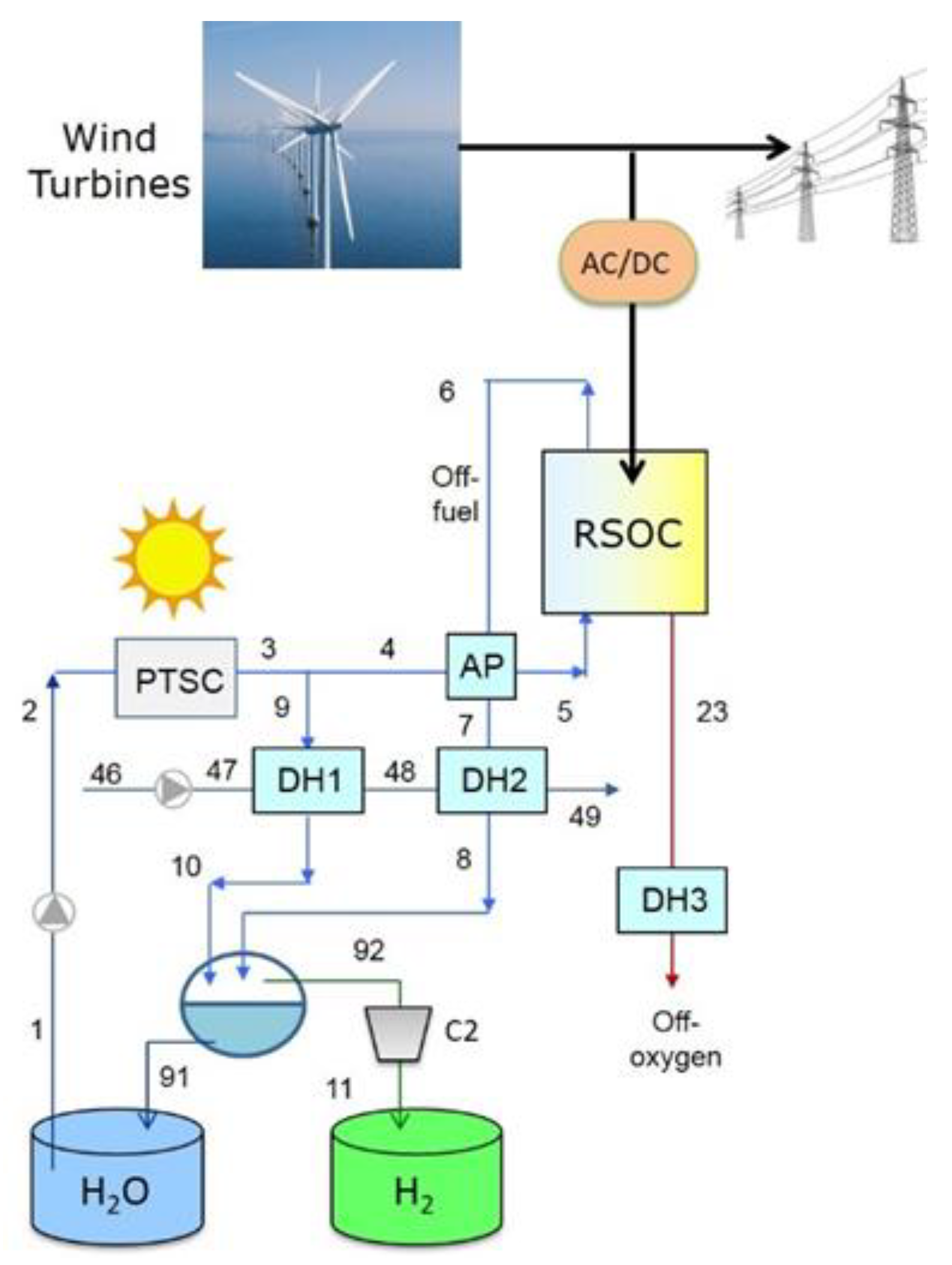
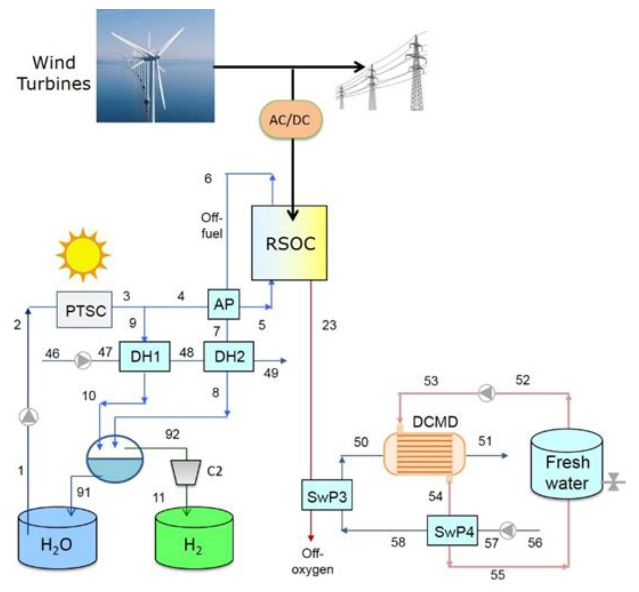
Figure 3 presents the proposed plant scheme in this study. As shown, PTSC preheats the water to 350 °C (node 3) before entering the anode preheater (AP). In other words, it acts as a steam generator for the RSOC and this is the main reason why this study uses PTSC. As mentioned above the term anode refers to the fuel cell mode. The water (now steam) is preheated in the anode preheater to about 630 °C before entering the RSOC. The temperature of the off-fuel (node 6) is 750 °C, which is used to preheat the steam in the anode preheater. The off-fuel after the anode preheater (node 7) is then first cooled down in a district heating heat exchanger (DH2) and then is sent to a condenser for separating the H2 and H2O. It shall be noted that the off-fuel after the RSOC is a mixture of H2 and H2O. This mixture depends on the utilization factor of the RSOC. The higher the utilization factor is the lower the amount of water in the mixture will be. The hydrogen and water mixture (off-fuel) after the RSOC is separated at 100 °C.
The design extracts some of the steam generated by the PTSC for the district heating (heat exchanger denoted as DH1 in the figure). The reason for this extraction is to regulate the temperature of the steam entering the RSOC. This is another reason why the proposed design uses a solar collector to generate steam. Later on, the analysis shows that the amount of this extraction is very important when wind velocity varies. The off-oxygen after the RSOC, which is separated from the steam in the RSOC (node 23), has a temperature of about 750 °C. One can use such hot stream for different purposes such as generating heat for the district heating (DH3) network, generating cooling for the district cooling network, or producing fresh water from a distillation unit (DCMD in this study). Thus, such designs offers a variety of possibilities depending on the location where the plant is to be installed. The operating temperature of DCMD is assumed to be 80 °C allowing 10 °C for the pinch temperature then off-oxygen is cooled down to 90 °C.
The driving forces of the RSOC is the excess energy from the wind turbines. In Denmark, the installed wind turbines are getting larger and larger and therefore in many hours of the year the electricity produced by the wind energy exceeds the demand. The suggested plant uses this excess electricity to generate fuel and at the same time, some other useful production. The study assumes a thermo-neutral voltage for all simulations carried out. This means that depending on the power supplied to the electrolyser, the cell voltage varies so that there is no need to supply heat to the electrolyser. Note that if the cell voltage is lower than the thermo-neutral voltage then the electrolyser needs heat at a very high temperature, which is not feasible.
The supply temperature for the district heating is 100 °C while its return temperature is 50 °C. These values are based on the current technology in Denmark. New generation district heating under development will have supply temperature at about 50 °C to 60 °C.
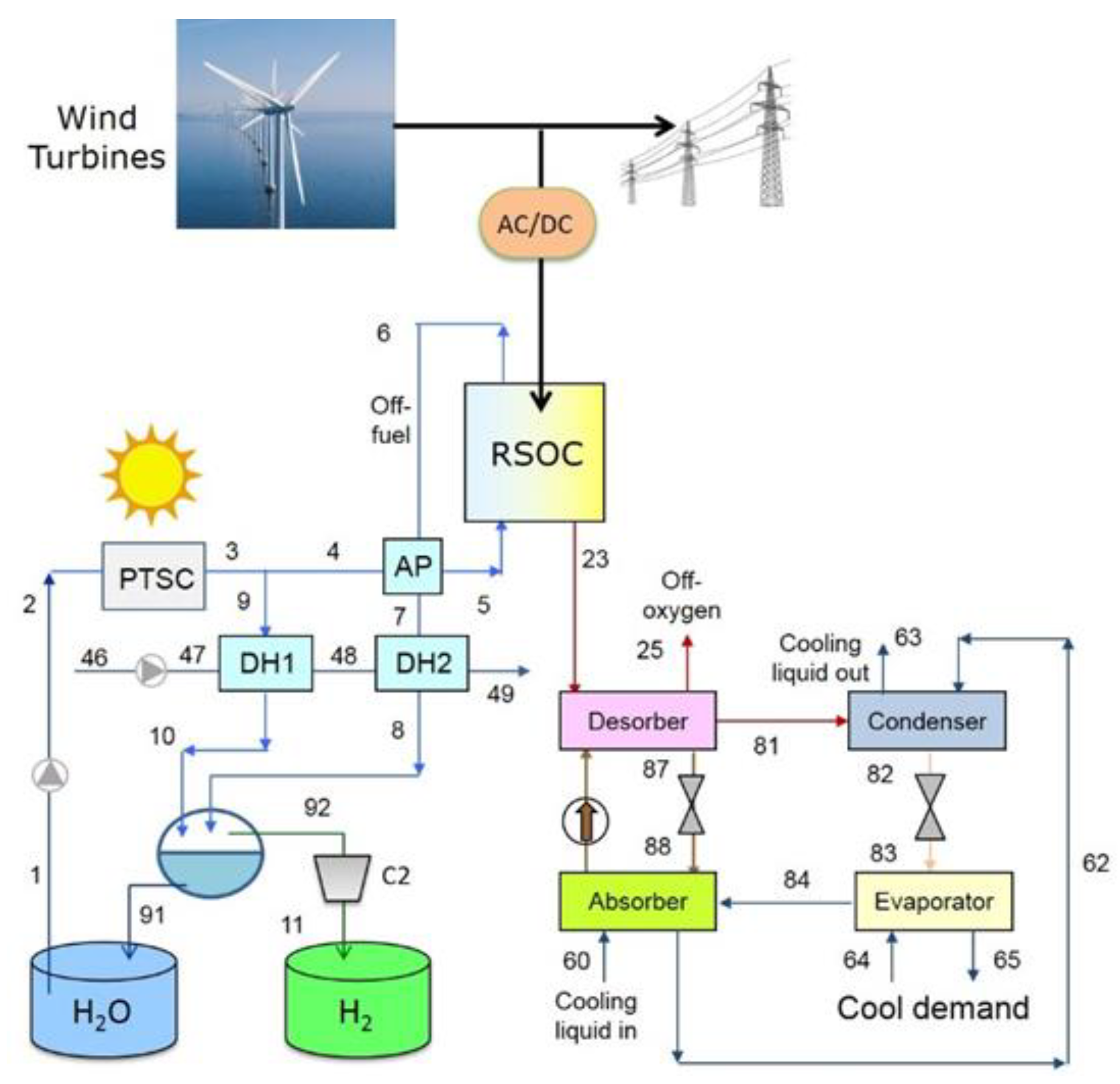
An alternative plant design replaces the DH3 in the off-oxygen stream with an absorption chiller, as shown in Figure 4. This plant is able to produce cooling (in addition to the heating) whenever cooling is needed, e.g. during summertime if located in a colder region, or year around if located in a warm region. Note that this particular design uses DH1 and DH2 for domestic hot water production (showering, washing, etc.). Therefore, such a combination provides many opportunities depending on the location of the plant.
A third alternative is proposed in Figure 5, wherein the absorption chiller is replaced with a DCMD unit to produce fresh water. Fresh water is becoming scarce in many areas and the need for such units is becoming more and more important, and therefore it is studied here.
The efficiency defined above (Equation (9)) does not take account the heat production, cool production and fresh water production. It only defines fuel production. Therefore, there is a need to define a new efficiency, which accounts for other production besides the fuel production (Qprod). Thus, the following efficiency is defined:
Such a definition calls for plant energy efficiency or plant utilization efficiency. Another point to be mentioned is that the solar energy is free and therefore one can assume that its contribution to the efficiency can be neglected. Therefore, the following efficiencies can be defined:
Obviously, the plant efficiency according to Equation (20) may be larger than unity under certain circumstances and the reason is that it neglects the free heat input from the solar energy to the system. In this study Qprod is then the summation of heat production, cool production and freshwater production as:
4. Results and Discussions
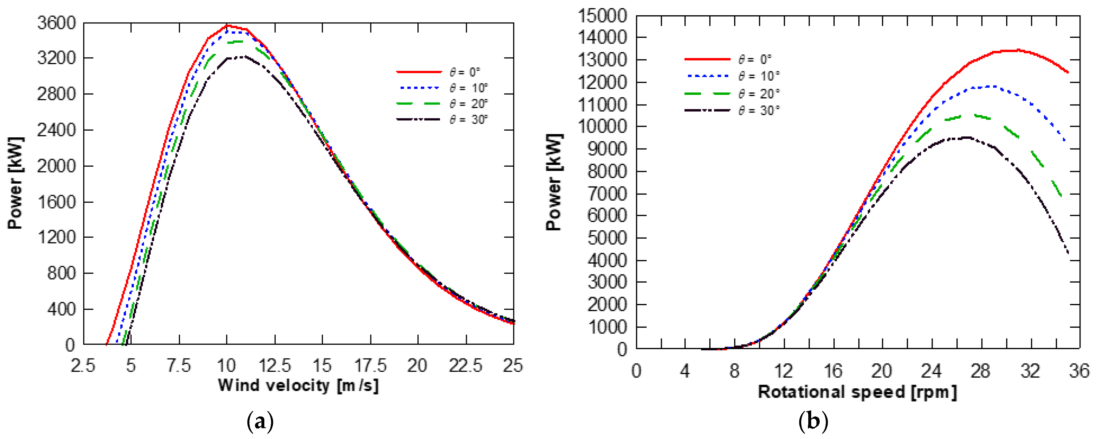
Figure 6 presents wind turbine performance curves. It shows that for any design there exists a wind velocity for which the power output is maximum (Figure 6a). It also demonstrates that for each design and at a constant wind velocity there exists a rotational speed for which turbine power is maximum (Figure 6b).
The figure also indicates that wind power decreases when the wind velocity is above 12 m/s (the default value for the present design). Another conclusion is that for each pitch angle there is a rotational speed at which the power is maximized. This indicates that to operate the wind turbines at their peak efficiency one needs to design a variable shaft speed, but at the expense of additional cost. It should be noted that for safety reasons, most companies also design the wind power in a way that when the power reaches its maximum then the rational speed is kept constant and does not respond to additional wind speed increases. Such a design avoids mechanical fracture, damage and failure of the blades. However, this study does not take this into account for structural modelling. The wind turbines does not respond to wind powers below about 5–6 m/s as shown in Figure 6a.
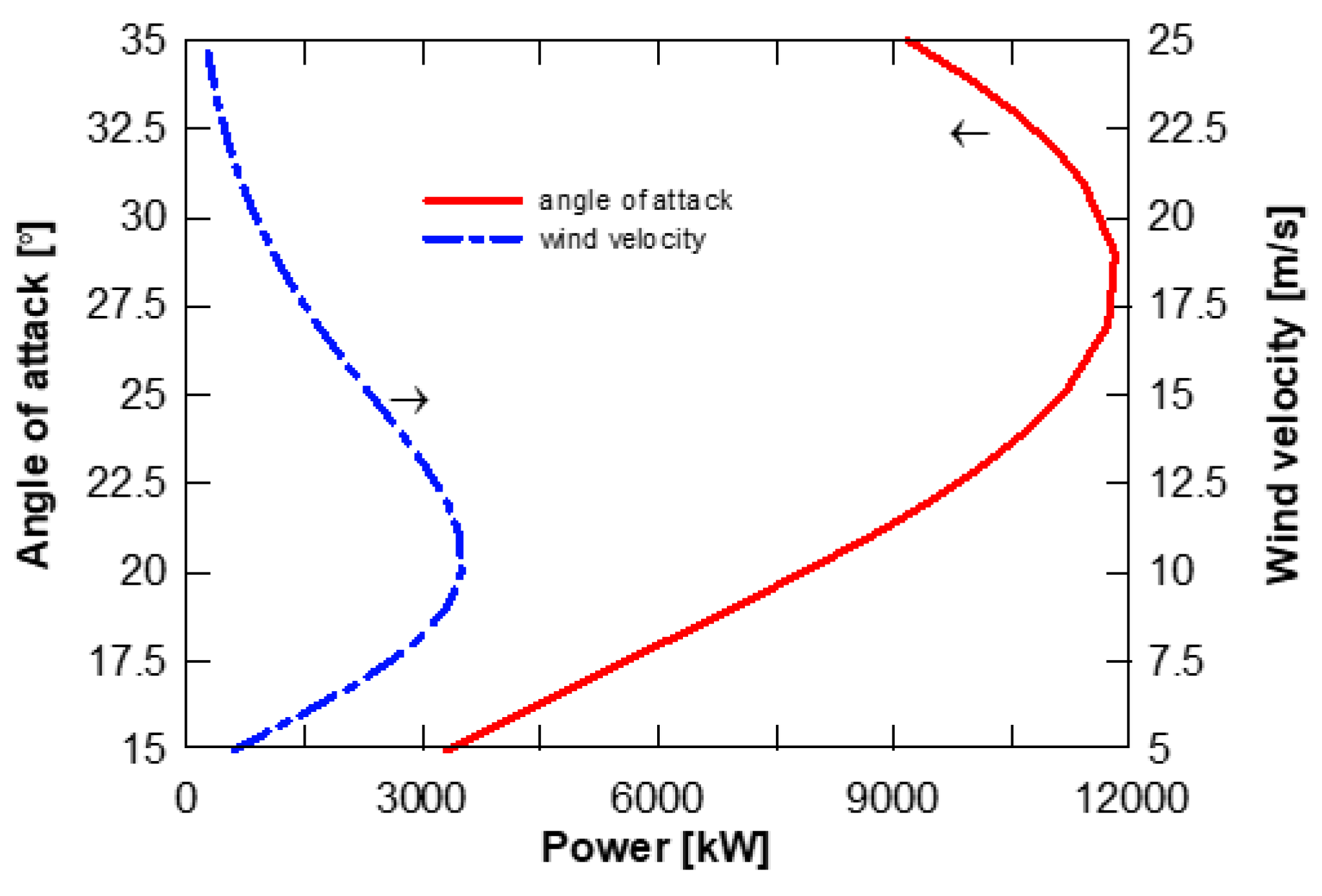
Figure 7 shows the optimum power of a wind turbine for different wind velocities and attack angles. As seen, the power is maximized at a wind velocity of 10 m/s and an attack angle of about 30°. Therefore, hereafter all calculations consider these values.
4.1. Plant with District Heating Only
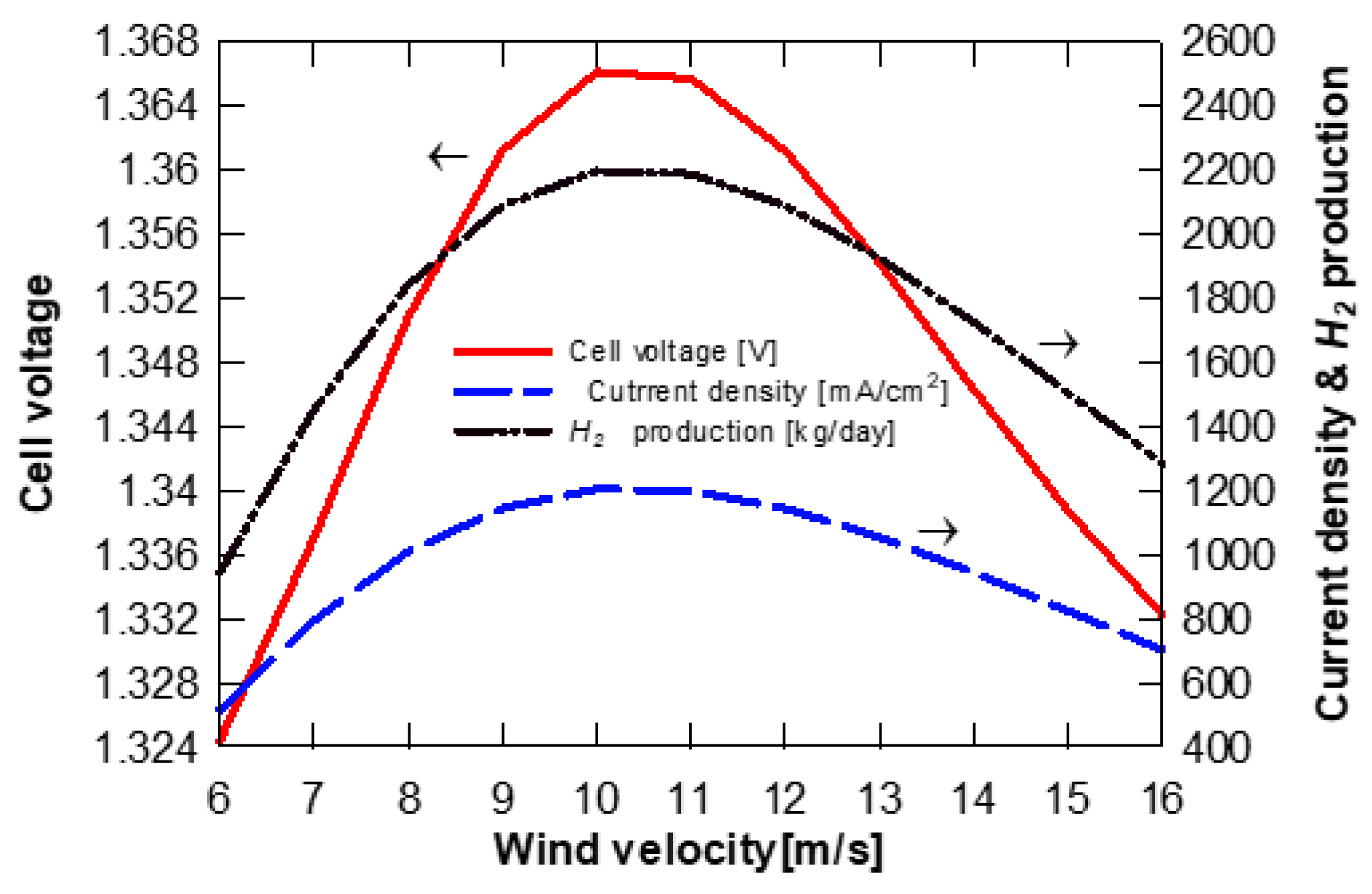
As demonstrated above, wind velocity is an important parameter for investigation, due to the power coefficient of the wind turbines. Wind turbines’ electrical power strongly depends on the wind power (wind speed) which directly affects the hydrogen production through the electrolyser system. Figure 8 presents the SOEC performance when the wind speed is changed.
As demonstrated above, the power of the turbine first increases to maximize at about 10 m/s (wind velocity) and then starts to decrease at wind velocities higher than about 11 m/s and therefore the power feed to the electrolyser is maximized at a wind velocity of about 10 m/s (parabolic shape). This results in a parabolic shape of the current densities as well as cell voltage. The current density and cell voltage increase when wind velocity increases from 6 m/s to 10 m/s. On the other hand, the current density and cell voltage decrease when the wind velocity is above 10 m/s. The current density and cell voltage reach 1208 mA/cm2 and 1.366 V, respectively, when the wind velocity is 10 m/s. We note also that this study takes into account the thermo-neutral voltage (no heat supplied to the electrolyser) and calculates this voltage. Since power supplied to the electrolyser decreases at wind velocities above 10 m/s, then hydrogen production first increases from 945 kg/day to maximize to 2197 kg/day and then starts to decrease and reaches to 1287 kg/day when the wind velocity is 16 m/s.
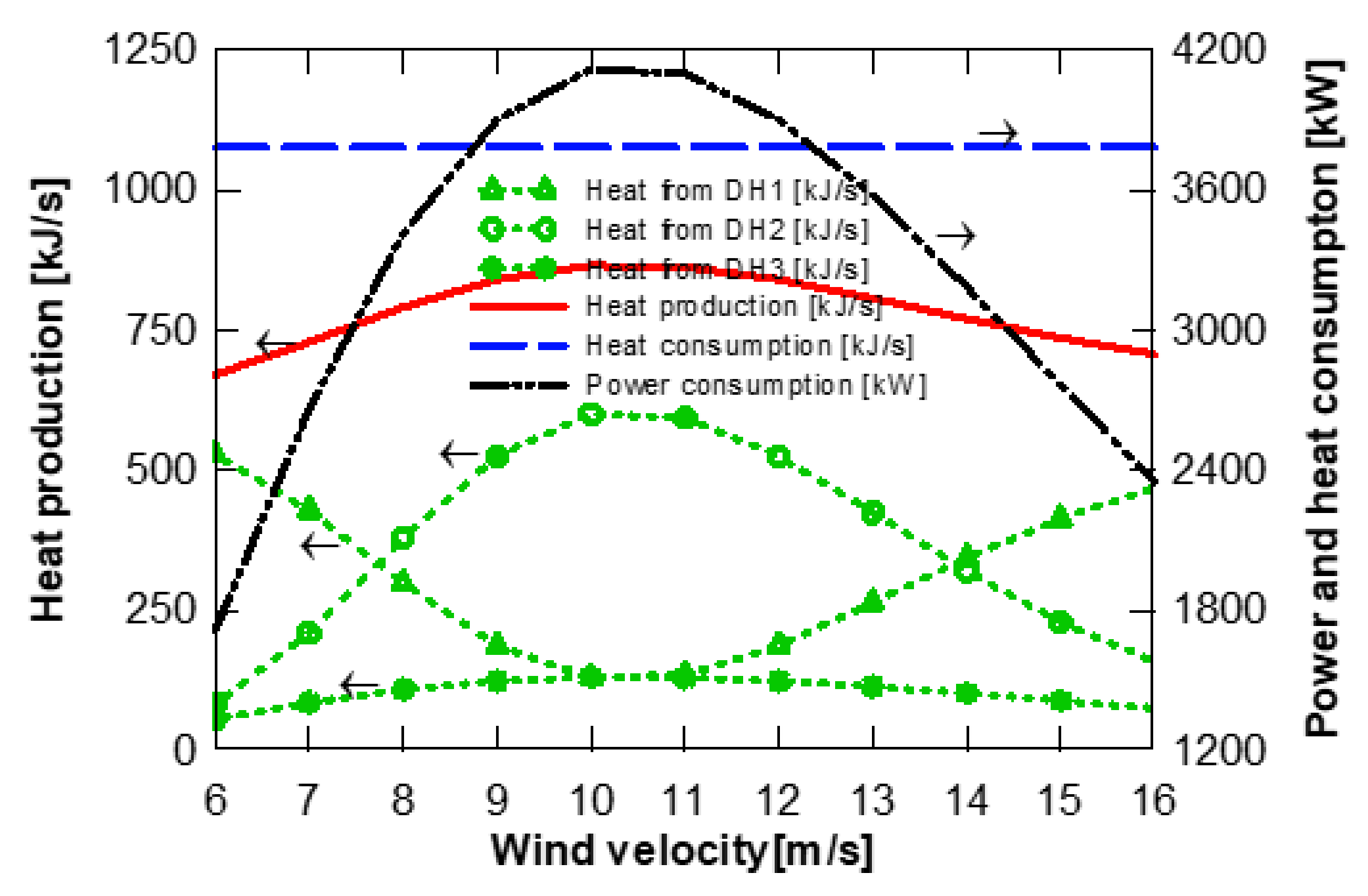
Figure 9 displays heat production as well as heat and power consumptions by the system with district heating only (c.f. Figure 3). Note that plant heat consumption is due to the solar energy through the PTSC while the plant power consumption is coming from wind turbines. Heat consumption through the PTSC (from solar energy) is constant since the number of PTSCs does not change and the temperature out of the PTSC is constant at 350 °C. The plant power consumption varies with the wind velocity and maximizes at 10 m/s which is about 4115 kW.
Plant total heat production (for district heating) shows a similar pattern (behaviour) as the power supplied to the electrolyser. Heat production maximizes at a wind velocity of 10 m/s, which is 865 kJ/s. Such a pattern of behaviour of the heat production is mainly due to the heat production of DH2, which is located at the off-hydrogen side and depends strongly on the electrolyser performance in terms of hydrogen production. Thus, heat production from DH2 located at the off-fuel side of the electrolyser increases/decreases as a direct consequence when the electricity supplied to the SOEC increases/decreases. Thus, heat production by DH2 is maximized when the wind velocity is 10 m/s (601 kJ/s). The reason is that steam production (mass flow) of the PTSC is constant (constant size and solar radiation) and therefore more steam goes through electrolysis as power to the electrolysis increases. This in turns means that less steam goes through the splitter just after the PTSC. Lower steam through this splitter causes less heat production through the DH1, which happens when the wind velocity increases from 6 m/s to 10 m/s, meaning that there exists less excess of steam for DH1. In other words, DH1 produces more heat as the electrolyser performance decreases. It is now obvious why the design includes a splitter after the PTSC. Further, heat production by DH1 is minimized when the wind velocity is 10 m/s (132 kJ/s). Heat production by DH3 (located on the off-oxygen side) strongly depends on the electrolysis performance, as better performance means more mass flow of off-oxygen. It is maximized when the wind velocity is 10 m/s (132 kJ/s).
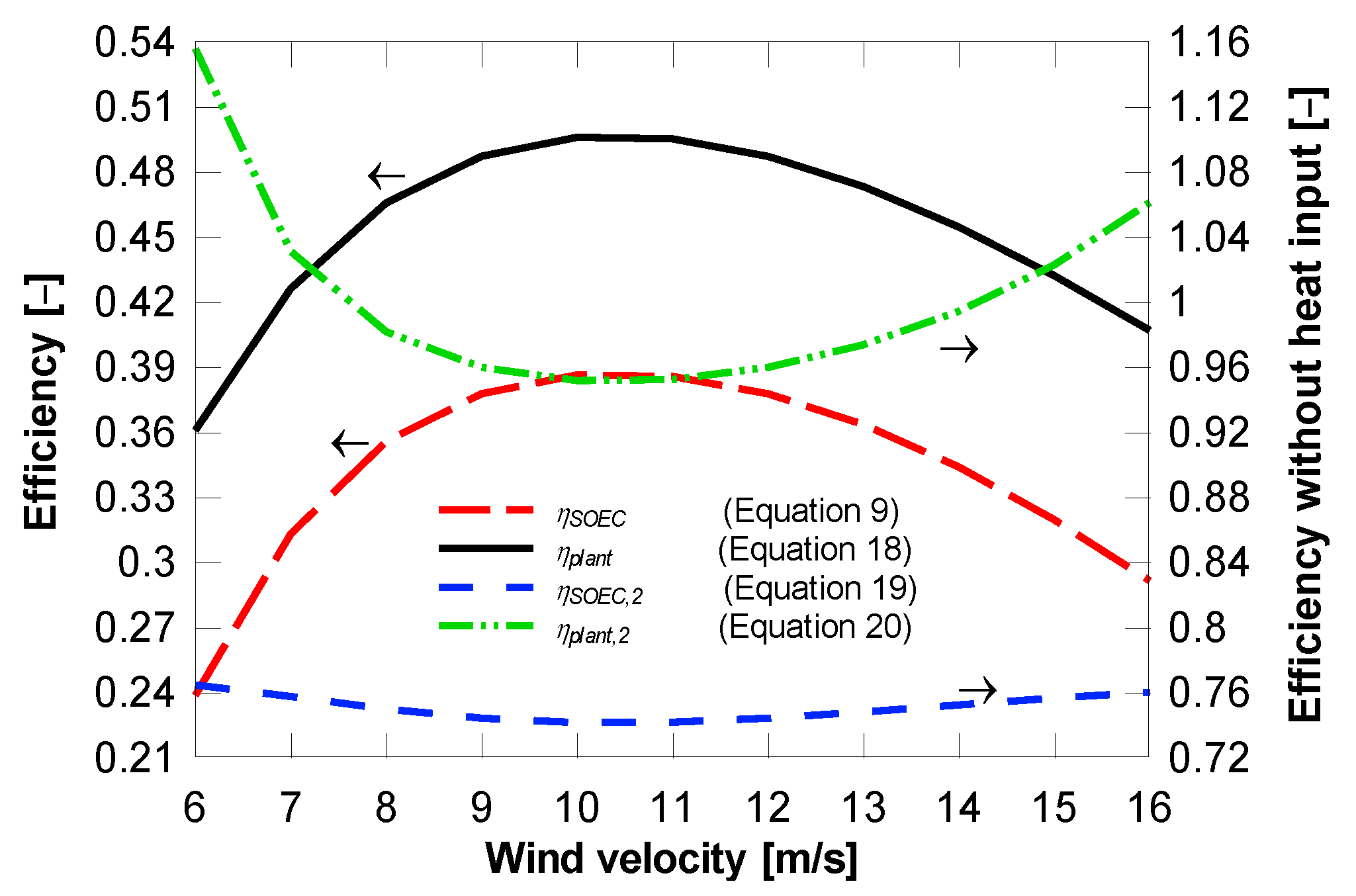
Figure 10 exhibits the electrolyser system efficiency as well as the plant efficiency when heating production is included. Plant performance in terms of efficiencies maximizes when the wind velocity is 10 m/s (Equations (9) and (18)). Electrolysis efficiency (Equation (9)) or hydrogen production efficiency increases from 24% to 39% when the wind velocity increases from 6 m/s to 10 m/s. Increasing the wind velocity from 10 m/s to 16 m/s causes the hydrogen efficiency to decrease from 39% to 29%. Similarly, the plant efficiency (Equation (18)) maximizes when the wind velocity is 10 m/s to reach a value of about 50%. On the other hand, neglecting the heat input by the solar energy (free heat) causes the plant performance to have a minimum value when the wind velocity is 10 m/s. Electrolyser efficiency (Equation (19)) or hydrogen production efficiency decreases from 76% to about 74% when the wind velocity increases from 6 m/s to 10 m/s. Further increases in wind velocity increase the hydrogen production efficiency back to 76% when the wind velocity reaches 16 m/s. However, such a variation is small and negligible. The minimum plant energy efficiency (Equation (20)) is about 95%, which happens when the wind velocity is 10 m/s. These results are encouraging and demonstrate the importance of including renewable energy systems in current energy systems.
As mentioned above, the supply temperature to the district heating network is 100 °C (current and most used technology). This indicates that some energy is lost from the system without being recovered. Decreasing the DH supply temperature to 50 °C (future DH generation under development) decreases the energy dissipation to the environment and thereby increases the plant efficiency. Note that Qprod in Equations (18) and (20) accounts for the summation of all heat generated for district heating (DH1, DH2 plus DH3).
As noted, the efficiency according to Equation (20) can be larger than 100% because this equation neglects the heat added to system from the solar energy (which varies from 95% to 115%). Including this free heat, the plant efficiency varies from 36% to about 50%, depending on the wind velocity.
4.2. Plant with District Heating and Cooling
The results for the plant with both DH and an absorption chiller are revealed in Figure 11.
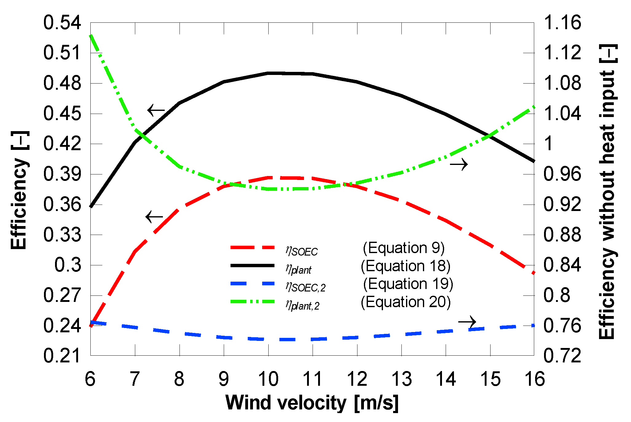
Off-air after the desorber is dissipated at 90 °C, well above the dew point. Now, Qprod in Equations (18) and (20) accounts for the summation of heat and cool generation. Multiplying the mass flow of the cooling flow with the enthalpy difference over the evaporator, we can calculate the generated cooling effect. The results obtained here are very similar to the previous case. SOEC hydrogen production and plant efficiencies (Equations (9) and (18)) are maximized when the wind speed is 10 m/s while neglecting the free energy from the Sun then these efficiencies (Equations (19) and (20)) is minimized when the wind speed is 10 m/s.
4.3. Plant with District Heating and Freshwater
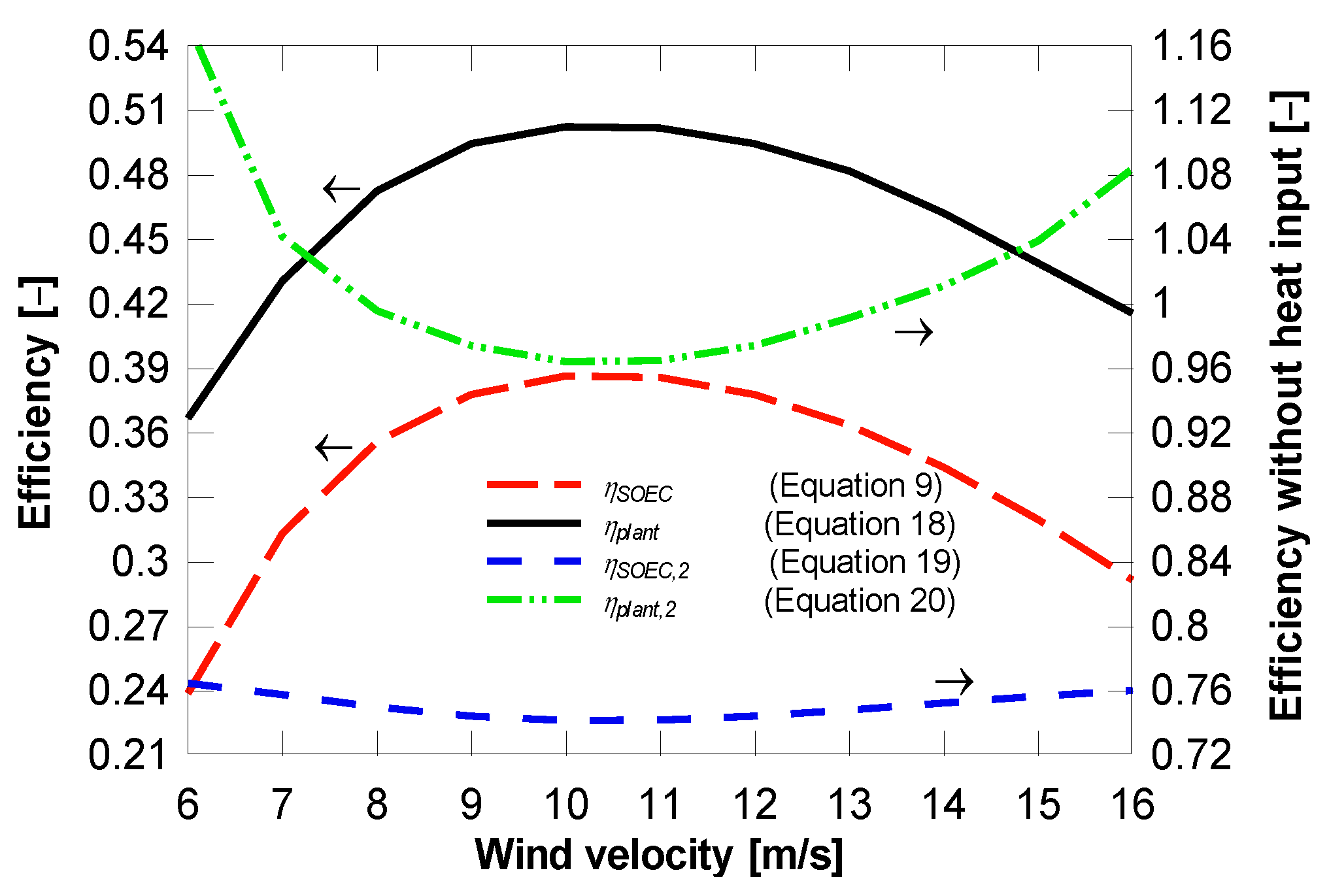
Figure 12 demonstrates the results obtained here from a plant, which generates both heat and fresh water in addition to producing hydrogen (c.f. Figure 5). Again, the results are similar as for the previous case, signifying that the definition in Equations (18) and (20) can be used for all polygeneration systems.
In this case, Qprod in Equations (18) and (20) is the summation of heat and fresh water generation. Since the fresh water production (kg/s) does not have the same dimensions as the heat (J/s) then this study defines the fresh water generation (J/s) as the energy difference between the inlet and outlet of the DCMD, which is the energy difference between the produced fresh water out of the DCMD and input water to the DCMD,
Similarly for seawater one would have:
and finally the performance of DCMD can be defined as:
Finally, the performance of the absorption chiller is calculated to be 0.617, which is the ratio between the heat released in the evaporator (cooling effect) over the heat absorbed in the desorber. The performance of the DCMD is calculated to be 0.934, which is the ratio between the heat absorbed by the fresh water, and the heat lost by the seawater in the DCMD (defined above).
As noted above, wind velocity has a significant effect on the plant performance. On the other hand, the solar radiation changes significantly during a day and therefore, it may have some effect on the plant performance. Therefore, a dynamic model may better capture plant performance by knowing solar radiation and wind velocity hour per hour for a specified location. Such data are usually available from the weather data for the region where the plant is to be placed.
4.4. Effect of Solar Radiation
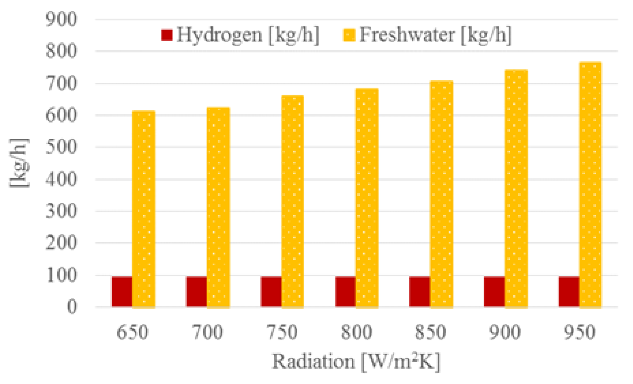
Since the plant utilizes a PTSC to generate steam then the effect of solar radiation on hydrogen fresh water production is also studied, see Figure 13. As documented, increasing the solar input energy increases fresh water production while hydrogen production remains almost unchanged. The reason is that wind power is constant and therefore power input to the electrolyser does not change. Consequently, the hydrogen production remains also unchanged while due to the higher solar radiation more steam will be generated which bypasses the separator before the cathode preheater (c.f. Figure 3). Note that in this case the DH in Figure 3 are replaced with DCMDs.
5. Conclusions
A polygeneration power-to-gas system based on reversible solid oxide cells is presented and analysed for hydrogen, heat, cool and fresh water production. The suggested plant utilizes a PTSC to generate steam for the electrolyser. The plant is able to produce 2200 kg of hydrogen per day when the wind velocity is 10 m/s. The analysis shows that the RSOC hydrogen production efficiency and plant energy efficiency reach about 39% and 47%, respectively, when the solar energy input into the system is accounted for. Neglecting the free heat input from solar energy to the system increases the RSOC efficiency to about 74% (hydrogen production only) and accounting for all products (hydrogen, heat and cooling), the plant efficiency reaches about 100%.
Conflicts of Interest
The author declares no conflicts of interest.
Nomenclature
| Symbol | Meaning (unit) |
| A | Area (m2) |
| Cp | Power coefficient (Equation (14)) |
| E | Voltage (V) |
| J | Current (A) |
| h | Enthalpy (J·kg−1) |
| Mass flow (kg·s−1) | |
| N | Number (–) |
| n | Angular velocity [rpm] |
| P | Power (W) |
| p | Pressure (N·m−2) |
| Q | Heat (J/s) |
| R | Rotor radius (m) |
| S | Swept area (m2) |
| T | Temperature (K) or (°C) |
| U | Heat transfer coefficient (W·m−2) |
| uw | Wind velocity (m·s−1) |
| W | Work (W) |
| w | Angular rotation (rad·s−1) |
| Greek letters | |
| Letter | Meaning (unit) |
| η | Efficiency (–) |
| λ | Tip speed ratio (rad) |
| Pitch angle (°) | |
| ρ | Density (kg·s−1) |
| Δ | Difference |
| Abbreviations | |
| Abbreviation | Meaning |
| DCMD | Direct contact membrane distillation |
| LHV | Lower heating value (J·kg−1) |
| RSOC | Reversible solid oxide cell |
| Subscripts | |
| Subscript | Meaning |
| amb | Ambient |
| act | Activation |
| cons | Concentration |
| ohm | Ohmic |
| prod | Production |
| rom | Mean at the outer surface |
| SOEC | Solid oxide electrolysis cell |
References
- Ni, M.; Leung, M.K.; Leung, D.Y. Technological development of hydrogen production by solid oxide electrolyzer cell (SOEC). Int. J. Hydrogen Energy 2008, 33, 2337–2354. [Google Scholar] [CrossRef]
- Zhang, X.; O’Brien, J.E.; O’Brien, R.C.; Housley, G.K. Durability evaluation of reversible solid oxide cells. J. Power Sources 2013, 242, 566–574. [Google Scholar] [CrossRef]
- Abuadala, A.; Dincer, I. Exergoeconomic analysis of a hybrid system based on steam biomass gasification products for hydrogen production. Int. J. Hydrogen Energy 2011, 36, 12780–12793. [Google Scholar] [CrossRef]
- Jensen, S.H.; Sun, X.; Ebbesen, S.D.; Knibbe, R.; Mogensen, M. Hydrogen and synthetic fuel production using pressurized solid oxide electrolysis cells. Int. J. Hydrogen Energy 2010, 35, 9544–9549. [Google Scholar] [CrossRef]
- Viviani, M.; Canu, G.; Carpanese, M.P.; Barbucci, A.; Sanson, A.; Mercadelli, E.; Nicolella, C.; Vladikova, D.; Stoynov, Z.; Chesnaud, A.; et al. Dual cells with mixed protonic-anionic conductivity for reversible SOFC/SOEC operation. Energy Procedia 2012, 2, 182–189. [Google Scholar] [CrossRef]
- Dillig, M.; Leimert, J.; Karl, J. Planar High Temperature Heat Pipes for SOFC/SOEC Stack Applications. Fuel Cells 2014, 14, 479–488. [Google Scholar] [CrossRef]
- Koytsoumpa, E.I.; Bergins, C.; Buddenberg, T.; Wu, S. The Challenge of Energy Storage in Europe: Focus on Power to Fuel. ASME Energy Resour. Technol. 2016, 138, 042002. [Google Scholar] [CrossRef]
- Chen, Z.; Zhang, Y.; Ji, T.; Li, C.; Xu, Z.; Cai, Z. Economic dispatch model for wind power integrated system considering the dispatchability of power to gas. IET Gener. Transm. Distrib. 2019, 13, 1535–1544. [Google Scholar] [CrossRef]
- Peters, R.; Baltruweit, M.; Grube, T.; Samsun, R.C.; Stolten, D. A techno economic analysis of the power to gas route. J. CO2 Util. 2019, 4, 616–634. [Google Scholar] [CrossRef]
- Schemme, S.; Samsun, R.C.; Peters, R.; Stolten, D. Power-to-fuel as a key to sustainable transport systems—An analysis of diesel fuels produced from CO2 and renewable electricity. Fuel 2017, 205, 198–221. [Google Scholar] [CrossRef]
- Mazza, A.; Bompard, E.; Chicco, G. Applications of power to gas technologies in emerging electrical systems. Renew. Sustain. Energy Rev. 2018, 92, 794–806. [Google Scholar] [CrossRef]
- Kouchachvili, L.; Entchey, E. Power to gas and H2/NG blend in SMART energy networks concept. Renew. Energy 2018, 122, 456–464. [Google Scholar] [CrossRef]
- Vo, T.T.; Xia, A.; Wall, D.M.; Murphy, J.D. Use of surplus wind electricity in Ireland to produce compressed renewable gaseous transport fuel through biological power to gas systems. Renew. Energy 2017, 105, 495–504. [Google Scholar] [CrossRef]
- Liu, W.; Wang, D.; Yu, X.; Jia, H.; Wang, W.; Yang, X.; Zhi, Y. Optimal of multi-source microgrid considering power to gas technology and wind power uncertainty. Energy Procedia 2017, 143, 668–673. [Google Scholar] [CrossRef]
- Collet, P.; Flottes, E.; Favre, A.; Raynal, L.; Pierre, H.; Capela, S.; Peregrina, C. Techno-economic and Life Cycle Assessment of methane production via biogas upgrading and power to gas technology. Appl. Energy 2017, 192, 282–295. [Google Scholar] [CrossRef] [Green Version]
- Koytsoumpa, E.I.; Karellas, S.; Kakaras, E. Modelling of Substitute Natural Gas production via combined gasification and power to fuel. Renew. Energy 2019, 135, 1354–1370. [Google Scholar] [CrossRef]
- Burgoyne, A.; Vahdati, M.M. Direct Contact Membrane Distillation. Desalin. Water Treat. 2000, 35, 1257–1284. [Google Scholar] [CrossRef]
- Shirazi, M.M.A.; Kargari, A.; Shirazi, M.J.A. Direct contact membrane distillation for seawater desalination. Sep. Sci. Technol. 2012, 49, 368–375. [Google Scholar] [CrossRef]
- Suárez, F.; Ruskowitz, J.A.; Tyler, S.W.; Childress, A.E. Renewable water: Direct contact membrane distillation coupled with solar ponds. Appl. Energy 2015, 158, 532–539. [Google Scholar] [CrossRef] [Green Version]
- Nakoa, K.; Date, A.; Akbarzadeh, A. DCMD modelling and experimental study using PTFE membrane. Desalin. Water Treat. 2016, 57, 3835–3845. [Google Scholar] [CrossRef]
- Cath, T.Y.; Adams, V.D.; Childress, A.E. Experimental study of desalination using direct contact membrane distillation: A new approach to flux enhancement. J. Membr. Sci. 2003, 228, 5–16. [Google Scholar] [CrossRef]
- Akikur, R.K.; Saidur, R.; Ping, H.W.; Ullah, K.R. Performance analysis of a co-generation system using solar energy and SOFC technology. Energy Convers. Manag. 2014, 79, 415–430. [Google Scholar] [CrossRef]
- Ni, M.; Leung, K.H.; Leung, D.Y.C. Energy and exergy analysis of hydrogen production by solid oxide steam electrolyzer plant. Int. J. Hydrogen Energy 2007, 32, 4648–4660. [Google Scholar] [CrossRef]
- Rokni, M. Thermodynamic analyses of municipal solid waste gasification plant integrated with solid oxide fuel cell and Stirling hybrid system. Int. J. Hydrogen Energy 2015, 40, 7855–7869. [Google Scholar] [CrossRef] [Green Version]
- Hernández-Pacheco, E.; Singh, D.; Nutton, P.N.; Patel, N.; Mann, M.D. A macro-level model for determining the performance characteristics of solid oxide fuel cells. J. Power Sources 2004, 138, 174–186. [Google Scholar] [CrossRef]
- Kim, Y.D.; Thu, K.; Ghaffour, N.; Ng, K.C. Performance investigation of a solar-assisted direct contact membrane. Membr. Sci. 2013, 427, 345–364. [Google Scholar] [CrossRef] [Green Version]
- Franchinia, G.; Notarbartolo, E.; Padovan, L.E.; Perdichizzi, A. Modeling, Design and Construction of a Micro-scale Absorption Chiller. Energy Procedia 2015, 82, 577–583. [Google Scholar] [CrossRef] [Green Version]
- de Vega, M.; Almendros-Ibanez, J.A.; Ruiz, G. Performance of a LiBr–water absorption chiller operating with plate heat exchangers. Energy Convers. Manag. 2006, 47, 3393–3407. [Google Scholar] [CrossRef] [Green Version]
- Porumb, R.; Porumb, B.; Balan, M. Numerical investigation on solar absorption chiller with LiBr-H2O operating conditions and performances. Energy Procedia 2017, 112, 108–117. [Google Scholar] [CrossRef]
- Misra, R.D.; Sahoo, P.K.; Gupta, A. Thermoeconomic Optimization of a LiBr/H2O Absorption Chiller Using Structural Method. Energy Resour. Technol. 2005, 127, 119–124. [Google Scholar] [CrossRef]
- Patek, J.; Klomfar, J. A computationally effective formulation of the thermodynamic properties of LiBr-H2O solutions from 273 to 500 K over full composition range. Int. J. Refrig. 2006, 29, 566–578. [Google Scholar] [CrossRef]
- Manyonge, A.W.; Ochieng, R.; Onyango, F.; Shichikha, J. Mathematical modelling of wind turbine in a wind energy conversion system: Power coefficient analysis. Appl. Math. Sci. 2012, 6, 4527–4536. [Google Scholar]
- Odeh, S.D.; Morrison, G.L.; Behnia, M. Modeling of parabolic trough direct steam generation solar collectors. Sol. Energy 1998, 62, 395–406. [Google Scholar] [CrossRef]
- Duffie, J.A.; Beckman, W.A. Solar Engineering of Thermal Processes, 4th ed.; John Wiley and Sons: Hoboken, NJ, USA, 2013; ISBN 978-1-118-41541-2 (ebk). [Google Scholar]
- Nellis, G.; Klein, S. Heat Transfer; Cambridge Press: Cambridge, UK, 2009; ISBN 978-0-521-88107-4. [Google Scholar]
- Gungor, K.E.; Winteron, R.H.S. A general correlation for flow boiling in tubes and annuli. Int. J. Heat Mass Transf. 1986, 29, 351–358. [Google Scholar] [CrossRef]
Figure 1.
Scheme of a DCMD plant. Seawater preheats first by freshwater (SwP4) and then by a heat source (SwP3).
Figure 1.
Scheme of a DCMD plant. Seawater preheats first by freshwater (SwP4) and then by a heat source (SwP3).

Figure 2.
Scheme of the absorption chiller.

Figure 3.
Scheme of the proposed plant with district heating. DH = district heating and AP = anode preheater.
Figure 3.
Scheme of the proposed plant with district heating. DH = district heating and AP = anode preheater.

Figure 4.
Scheme of the proposed plant with district cooling. DH = district heating and AP = anode preheater.
Figure 4.
Scheme of the proposed plant with district cooling. DH = district heating and AP = anode preheater.

Figure 5.
Scheme of the proposed plant with freshwater production. DH = district heating and AP = anode preheater.
Figure 5.
Scheme of the proposed plant with freshwater production. DH = district heating and AP = anode preheater.

Figure 6.
Wind turbine performance curves: (a) power vs wind velocity; (b) power vs rotational speed.
Figure 6.
Wind turbine performance curves: (a) power vs wind velocity; (b) power vs rotational speed.

Figure 7.
Wind turbine power response to wind velocities and attack angles.

Figure 8.
SOEC performance as function of wind velocity for plant with DH connection only (c.f. Figure 3).
Figure 8.
SOEC performance as function of wind velocity for plant with DH connection only (c.f. Figure 3).

Figure 9.
Heat production as function of wind velocity for plant with DH connection only (c.f. Figure 3).
Figure 9.
Heat production as function of wind velocity for plant with DH connection only (c.f. Figure 3).

Figure 10.
Plant performance as a function of wind velocity for the case with DH only (c.f. Figure 3).
Figure 10.
Plant performance as a function of wind velocity for the case with DH only (c.f. Figure 3).

Figure 11.
Plant performance as function of wind velocity for the case with DH and AP (c.f. Figure 4).
Figure 11.
Plant performance as function of wind velocity for the case with DH and AP (c.f. Figure 4).

Figure 12.
Plant performance as function of wind velocity for the case with DH and DCMD (c.f. Figure 5).
Figure 12.
Plant performance as function of wind velocity for the case with DH and DCMD (c.f. Figure 5).

Figure 13.
Fuel (H2) and fresh water production as a function of solar radiation.


Table 1.
Specifications for RSOC (anode and cathode referred to fuel cell mode).
| Parameter | Value |
|---|---|
| Anode thickness | 600 μm (nickel and yttria stabilized zirconia cermet) |
| Cathode thickness | 50 μm (strontium-doped lanthanum manganite) |
| Electrolyte thickness | 10 μm (yttria stabilized zirconia) |
| Cell area | 144 cm2 (12 cm × 12 cm) |
| Operating temperature | 750 °C |
| Porosity | 30% |
| Tortuosity | 2.5 |
| Nr. of cells per stack | 70 |
| Number of stacks | 200 |
Table 2.
Specifications of the DCMD (Direct Contact Membrane Desalination) hollow fibre module.
| Parameter | Value |
|---|---|
| Fibre length | 0.4 m |
| Inner diameter of fibre | 0.3 mm |
| Membrane thickness | 60 μm |
| Porosity | 75% |
| Membrane conductivity | 0.25 W/mK |
| Shell diameter | 0.003 m |
| Number of fibres | 3000 |
| Packing density | 60% |
| Inlet temperature | 80°C |
| Model Constants | |
| Ck | 15.18 × 10⁻⁴ |
| Cm | 5.1 × 10³ m−1 |
| Cp | 12.97 × 10⁻¹¹ m |
Table 3.
The main parameters for absorption chiller, basic case.
| Parameter | Value |
|---|---|
| Desorber gas outlet temperature | 90 °C |
| Rich solution | 0.593 |
| Week solution | 0.548 |
| Condenser outlet temperature | 32 °C |
| Rich solution pressure after valve | 0.008 bar |
| Absorber cooling inlet temperature | 15 °C |
| Solution pump pressure | 0.05 bar |
| Cooling deliver temperature | 4 °C |
| Cooling return temperature | 11 °C |
| Cooling flow pressure | 16 bar |
Table 4.
Wind turbine model specifications used in this study.
| Parameter | Value |
|---|---|
| Blade radius | 30 m |
| Hub height | 100 m |
| Rotational speed | 15 rpm |
| Angle of attack | 10° |
| Conversion efficiency | 0.85 |
| Number of wind turbines | 13 |
| Wind speed (default) | 10 m/s |
Table 5.
Main specifications for PTSC (Parabolic Trough Solar Collector).
| PTSC | Value |
|---|---|
| Length | 250 m |
| Number of rows | 10 |
| Receiver | |
| Diameters (Dri, Dro) | 33, 38 mm |
| Material | Stainless steel |
| Conductivity (kr) | 60 W/mK |
| Coating | Black Niquel |
| Emissivity (εr) | 0.06 |
| Absorptivity (α ) | 0.94 |
| Cover | |
| Diameters (Dci, Dco) | 84, 90 mm |
| Material | Glass |
| Conductivity (kc) | 0.035 W/mK |
| Emissivity (εc) | 0.84 |
| Transmissivity (τ ) | 0.94 |
| Air pressure in the gap (pm) | 0.5 mbar |
| Concentrator | |
| Reflectivity () | 0.93 |
| Intercept factor (γ ) | 0.93 |
| Aperture | 2.5 m |
| Incidence angle modifier (β ) | 1 |
| Manifold losses | 20% of the heat to ambient |
| Other Information | |
| Ambient temperature (Tamb) | 28 °C |
| Sky temperature (Tsky) | 20 °C |
| Wind velocity (Vwind) | 5 m/s |
| Saturation temperature (Tsat) | 80 °C (253 K) |
© 2019 by the author. Licensee MDPI, Basel, Switzerland. This article is an open access article distributed under the terms and conditions of the Creative Commons Attribution (CC BY) license (http://creativecommons.org/licenses/by/4.0/).
Share and Cite
MDPI and ACS Style
Rokni, M.M. Power to Hydrogen Through Polygeneration Systems Based on Solid Oxide Cell Systems. Energies 2019, 12, 4793. https://0-doi-org.brum.beds.ac.uk/10.3390/en12244793
AMA Style
Rokni MM. Power to Hydrogen Through Polygeneration Systems Based on Solid Oxide Cell Systems. Energies. 2019; 12(24):4793. https://0-doi-org.brum.beds.ac.uk/10.3390/en12244793
Chicago/Turabian StyleRokni, Marvin M. 2019. "Power to Hydrogen Through Polygeneration Systems Based on Solid Oxide Cell Systems" Energies 12, no. 24: 4793. https://0-doi-org.brum.beds.ac.uk/10.3390/en12244793
Note that from the first issue of 2016, this journal uses article numbers instead of page numbers. See further details here.