Transfer Path Analysis for Semisubmersible Platforms Based on Noisy Measured Data

Abstract

A new energy transfer path analysis (TPA) method that aims to analyze the transfer path of components with characteristic frequencies in semisubmersible platform structures is proposed in this paper. Due to the complexity of semisubmersible platforms, traditional TPA methods based on measurements are no longer applicable. In the proposed method, the structure is considered to be a “source-path-receiver” system and the vibration signals from the source-points are analyzed first to determine the characteristic components. Then, the signals from the source-points and the receiver-points are decomposed by introducing a state–space model. Through correlation functions, the characteristic components can be extracted, and the transfer path can be obtained by calculating the transmissibility functions. By using transmissibility functions, the proposed method only relies on the output responses and avoids the measurement of force and transfer functions. Three examples, one numerical example containing a two-degree-of-freedom (2-DOF) model and a 5-DOF model, one experiment implemented on a barge, and the data from a dynamic positioning (DP) cabin of a semisubmersible platform were used to investigate the performance of the proposed method. The results show that the proposed method can be used to assess the transfer path quantitatively and has potential value of application in engineering.

1. Introduction

With the transformation and upgrading of the marine engineering industry, the influence of vibration and noise generated by offshore platforms on the health of sea workers is receiving more and more attention. The International Maritime Organization (IMO) and various classification societies have strict control over the noise levels of the cabins. Through the analysis of vibration and the noise transfer path, the characteristics of excitation process can be reflected and proper vibration and noise reduction measures can be implemented. In addition, when a machine or equipment inside the platform fails, the characteristics of the measured signals will change. Therefore, the analysis of the transfer path helps to perform a state detection and fault diagnosis of the machine or equipment [1]. Therefore, the operating state of the machine can be obtained in time, and the fault can be accurately found. Consequently, the acoustic performance of the offshore platform can be improved.

When structure is in a real working environment, analyzing its energy transfer path is complicated and difficult [2]. TPA is a powerful method for the transfer analysis of vibration and noise [3]. In the traditional TPA method, by introducing the frequency response function (FRF) between the excitation and the response, the contribution of each path is defined. Therefore, the response at any point can be expressed by the excitation force and the path contributions [4]. By implementing the traditional TPA method, the relationship between the input and output responses can be estimated, and it mainly contains two steps: The first step is to measure the FRF, and, in the second step, the operation vibrations are measured [5]. The TPA method has already become a mature and reliable technique for solving the noise and vibration transfer path problems, but, in this technique, each path needs to be isolated by disassembling the system. When the system is disassembled, one applies a known force at the location where the subsystem of interest is linked with another subsystem. If one knows the force and the response, one can identify the transfer path. This measurement is very time-consuming, and the boundary conditions are no longer correct [6]. At the same time, this method is disadvantages in many practical cases since it requires large space and a strong support wall for the installation of the load cells [7]. Therefore, to solve this problem, many efforts have been made to indirectly measure the excitation force [8,9]. However, these improvements still have some problems in many practical situations.

Since the purpose of the TPA method is to determine the contribution of energy transfer in the system, to reduce the time and complexity of the measurement, the concept of transmissibility functions are introduced in the TPA method [10], which is called the OTPA method. In addition, Ribeiro et al. [11] generalized it in a multi-degree-of-freedom system. By using the transmissibility functions instead of the FRF, we can describe the transfer path from the perspective of contributions, which are determined by the responses among sensors. The stage of measuring forces is avoided, and no disassembly is required. Another advantage of the OTPA method is that, as long as the unit is normalized, various types of sensors, such as acceleration, velocity, sound presser, and even force, can be used for the measurement [12]. By this, the limitation of the test-time was overcome and the analysis process was accelerated. However, due to the complexity of platform, this method still has some limitations, such as the estimation error, the neglected path, and cross-coupling between input accelerations [13].

Due to the complex marine environment, marine structures, such as offshore platforms, are excited by various sources, and the response signals are strongly affected by the noise, disturbance, and additional forces. In addition, a platform has a large number of compartments, and the structural rigidity is large. The complexity of the structure makes it impossible to visually recognize the transmission path. Therefore, it is not easy to calculate the transfer path by using the existing methods. In 2019, Liu et al. [14] proposed an iterative noise extraction and elimination method to deal with noise contaminated measured signals and the interference of high-energy noise on modal parameter identification can be reduced significantly. By introducing a first order differential equation, the shortcomings of the traditional Prony method were overcome, and the accuracy was improved. Through this method, the high energy harmonic components can be well identified. This method is also applicable to the extraction of the characteristic components. By extracting the characteristic components of each receiver-point of the offshore platform, the transmission of the characteristic components can be studied.

In this paper, a new TPA method based on the extraction of the characteristic components and the transmissibility function is proposed. The vibration signals at the source-points and receiver-points are first measured. Then, by analyzing the signals from the source-points, the vibration of frequencies with time can be obtained and the characteristic components can be determined. To extract the characteristic components, two steps are implemented, i.e., signal decomposition by the complex exponential decomposition and a screening step by correlation analysis. By computing the transmissibility function of the characteristic component, the transfer path in the whole space can be identified. In this study, one numerical example (containing a 2-DOF system and a 5-DOF system), one experimental study on a barge, and one sea trial test for a semisubmersible platform were used to evaluate the performance of the proposed method.

2. Preliminaries

2.1. Transfer Path Analysis

TPA regards the entire system as having three parts, namely “source–path–receiver”, and the response at mth receiver-point can be expressed as:

$$y_m\left(t\right)=\sum _{i=1}^n{H}_{m,i}\left(t\right)·f_i\left(t\right)$$

(1)

where $y_m\left(t\right)$ is the response of the mth receiver-point, $f_i\left(t\right)$ is the excitation force on the ith source-point, and $H_{m,i}\left(t\right)$ is the transfer function between the ith source-point and the mth receiver-point. Equation (1) in the form of matrix can be expressed as:

$$\left[\begin{array}{cccc}{Y}_1& Y_2& \dots & Y_m\end{array}\right]=\left[\begin{array}{cccc}{F}_1& F_2& \dots & F_n\end{array}\right]\left[\begin{array}{cccc}{H}_{11}& H_{12}& \dots & H_{1m}\\ H_{21}& H_{22}& \dots & H_{2m}\\ ⋮& ⋮& \ddots & ⋮\\ H_{n1}& H_{n2}& \dots & H_{nm}\end{array}\right]$$

(2)

where $Y_j(j\le m)$ means the jth output of the system and $F_i(i\le n)$ means the ith input of the system. $H_{ij}$ means the transfer function of from $F_i$ to $Y_j$, which represents the transfer characteristic of the system.

2.2. Operational Transfer Path Analysis

In the OTPA method, the signals of input and output are measured under actual operating conditions [15]. The transfer function $\mathbf{H}$ changes to the transfer function under operating conditions $\mathbf{T}$:

$$\left[\begin{array}{cccc}{Y}_1& Y_2& \dots & Y_m\end{array}\right]=\left[\begin{array}{cccc}{F}_1& F_2& \dots & F_n\end{array}\right]\left[\begin{array}{cccc}{T}_{11}& T_{12}& \dots & T_{1m}\\ T_{21}& T_{22}& \dots & T_{2m}\\ ⋮& ⋮& \ddots & ⋮\\ T_{n1}& T_{n2}& \dots & T_{nm}\end{array}\right]$$

(3)

When calculating the transfer function $\mathbf{T}$, the inverse matrix method is used. By measuring under different operational conditions, multiple input and output data are obtained, and the transfer function $\mathbf{T}$ can be solved. Assume k different operation conditions are measured. Then, Equation (3) can be expressed as:

$$\left[\begin{array}{cccc}{Y}_1^1& Y_2^1& \dots & Y_m^1\\ Y_1^2& Y_2^2& \dots & Y_m^2\\ ⋮& ⋮& \ddots & ⋮\\ Y_1^k& Y_2^k& \dots & Y_m^k\end{array}\right]=\left[\begin{array}{cccc}{X}_1^1& X_2^1& \dots & X_n^1\\ X_1^2& X_2^2& \dots & X_n^2\\ ⋮& ⋮& \ddots & ⋮\\ X_1^k& X_2^k& \dots & X_n^k\end{array}\right]\left[\begin{array}{cccc}{T}_{11}& T_{12}& \dots & T_{1m}\\ T_{21}& T_{22}& \dots & T_{2m}\\ ⋮& ⋮& \ddots & ⋮\\ T_{n1}& T_{n2}& \dots & T_{nm}\end{array}\right]$$

(4)

where $X_i^p$ and $Y_i^p(p\le k)$ are the measured input and output under the ith operational condition. When $k\ge n$, the matrix has an inverse matrix, and the transfer coefficient $\mathbf{T}$ can be obtained. By this, we can obtain:

$${\mathbf{Y}}_i={\mathbf{X}}_i{\mathbf{T}}_{ij}$$

(5)

where ${\mathbf{X}}_i$ and ${\mathbf{Y}}_i$ are the matrices of the measured input and output, respectively.

3. The Energy Transfer Path Analysis Method Based on a State–Space Model and the Transmissibility Function

3.1. Sensor Installation and the Definition of Characteristic Components

In ocean engineering, the form of the structures plays an important role in the transmission of vibration and noise. Thus, when measuring the response, we should first make a preliminary subjective assessment based on the structural form and find suitable locations for sensor installation. According to the assessment, the accelerometer sensors are installed to form an array under some rules, and the signals on the receiver-points are received. In addition, the sensors should be installed on the source-points to receive the input signals. After measurement, the vibration signal $y_n\left(t\right)$ at the nth source-point and $x_m\left(t\right)$ at the mth receiver-point can be obtained.

Denoting time $t_k$ as $t_k=k\mathsf{\Delta }t$ where $\mathsf{\Delta }t$ means the sampling interval and a Hankel matrix ${\mathcal{C}}_n\left(k\right)$ can be introduced as [16]:

$${\mathcal{C}}_n\left(k\right)=\left[\begin{array}{cccc}{y}_{n,k}& y_{n,k+1}& \cdots & y_{n,k+\beta -1}\\ y_{n,k+1}& y_{n,k+2}& \cdots & y_{n,k+\beta }\\ ⋮& ⋮& \ddots & ⋮\\ y_{n,k+\alpha -1}& y_{n,k+\alpha }& \cdots & y_{n,k+\alpha +\beta -2}\end{array}\right]$$

(6)

where $\alpha$ and $\beta$ are the number of rows and columns of the matrix ${\mathcal{C}}_n\left(k\right)$. Then, by using the singular value decomposition (SVD), we can obtain a state matrix as:

$${\mathsf{\Lambda }}_n={\mathbf{S}}_{n,1}^{-1/2}{\mathbf{U}}_{n,1}^{\mathrm{T}}{\mathcal{C}}_n\left(1\right){\mathbf{V}}_{n,1}{\mathbf{S}}_{n,1}^{-1/2}$$

(7)

By this, the time–frequency spectrum of the signal at the source-point can be obtained, from which we can see the variation of the frequencies of the components. In addition, from the spectrum, the components with larger energy and more stable components can be observed. These components play a major role in the vibration of the system, and are considered as the characteristic components.

3.2. Relationship between Characteristic Component and Noise

The acceleration signal at the mth receiver-point can be expressed as:

$$x_m\left(t\right)=\sum _{i=1}^q{x}_{m,i}\left(t\right)+\sum _{j=1}^{q_c}{x}_{m,j}^c\left(t\right)$$

(8)

where $x_{m,j}^c$ and $x_{m,i}\left(t\right)$ mean the characteristic components and other components (i.e., noise, disturbances, and additional forces) at the mth point. $q_c$ and q mean the number of characteristic components and the number of other components. In addition, $x_m\left(t\right)$ can be decomposed as a sum form of a complex exponential function:

$$x_m\left(t\right)=\sum _{i=1}^q{\gamma }_{m,i}{e}^{{\lambda }_{m,i}t}+\sum _{j=1}^{q_c}{\gamma }_{m,j}^c{e}^{{\lambda }_{m,j}^{c}t}=\sum _{i=1}^{q+q_c}{\gamma }_{m,i}{e}^{{\lambda }_{m,i}t}$$

(9)

where ${\lambda }_{m,i}$ and ${\gamma }_{m,i}$ are the poles and the residues of the signal and ${\lambda }_{m,c}$ and ${\gamma }_{m,c}$ correspond to the characteristic component. Actually, one measured signal contains several characteristic components, but, in the proposed method, the transfer path of the characteristic components are calculated one by one. Thus, in the analysis below, we assume that the signal has only one characteristic component ($q_c=1$) to illustrate the algorithm and Equation (9) can be rewritten as:

$$x_m\left(t\right)=\sum _{i=1}^q{\gamma }_{m,i}{e}^{{\lambda }_{m,i}t}+{\gamma }_m^c{e}^{{\lambda }_m^{c}t}=\sum _{i=1}^{q+1}{\gamma }_{m,i}{e}^{{\lambda }_{m,i}t}$$

(10)

3.3. The Extraction of the Characteristic Component

After determining the relationship between the characteristic component and the noise components, we need to extract the characteristic component from the measured signal. At the mth receiver-point, the equally spaced sampled form of the signal $x_m\left(t\right)$ can be expressed as [17]:

$${\tilde{x}}_{m,k}\left(t\right)=\sum _{i=1}^q{\gamma }_{m,i}{e}^{{\lambda }_{m,i}k\mathsf{\Delta }t}+{\gamma }_m^c{e}^{{\lambda }_m^{c}k\mathsf{\Delta }t}=\sum _{i=1}^{q+1}{\gamma }_{m,i}{e}^{{\lambda }_{m,i}k\mathsf{\Delta }t}$$

(11)

Then, a Hankel matrix can be defined as:

$${\mathbf{H}}_m\left(k\right)=\left[\begin{array}{cccc}{x}_{m,k}& x_{m,k+1}& \cdots & x_{m,k+\eta -1}\\ x_{m,k+1}& x_{m,k+2}& \cdots & x_{m,k+\eta }\\ ⋮& ⋮& \ddots & ⋮\\ x_{m,k+\xi -1}& x_{m,k+\xi }& \cdots & x_{m,k+\xi +\eta -2}\end{array}\right]$$

(12)

with a dimension of $\xi \times \eta$. By implementing the SVD to $H\left(0\right)$ and $H\left(1\right)$, we can obtain:

$${\mathbf{A}}_m={\mathbf{S}}_{m,1}^{-1/2}{\mathbf{U}}_{m,1}^{\mathrm{T}}{\mathbf{H}}_m\left(1\right){\mathbf{V}}_{m,1}{\mathbf{S}}_{m,1}^{-1/2}$$

(13)

where ${\mathbf{A}}_m$ is the state matrix of the system. Assume the characteristic roots of ${\mathbf{A}}_m$ are $z_n$. Then, $\lambda$ can be calculated by $\lambda =ln{z}_n/\mathsf{\Delta }t$. Then, the ${\gamma }_{m,i}$ can be calculated. According to the definition of ${\lambda }_{m,i}$, the frequencies in Hz can be obtained by:

$$f_i=\frac{Im\left({\lambda }_{m,i}\right)}{2\pi }$$

(14)

where $Im$ means the imaginary part of ${\gamma }_{m,i}$. By comparing the frequencies that were calculated by Equation (14) and the frequency of the characteristic component, the components with similar frequencies as the characteristic component can be determined. Near the frequency of the characteristic component, there may be several corresponding components. From the corresponding ${\gamma }_{m,i}$ and ${\lambda }_{m,i}$, the component can be extracted as:

$$x_{m,l}\left(t\right)={\gamma }_{m,l}{e}^{{\lambda }_{m,l}k\mathsf{\Delta }t}$$

(15)

where $x_{m,l}$$(l=1,2,3,\dots )$ means the reconstructed signal at the mth point, whose frequency is near the frequency of the characteristic component.

3.4. Screening for the Characteristic Component

Since several components are extracted, a screening step is needed to choose the real one. Here, the screening step is implemented by calculating the correlation coefficient between the characteristic component $x_{m,c}\left(t\right)$ and the measurement signal $x_m\left(t\right)$ as:

$${\rho }_{x_{m,c}{x}_m}=\frac{cov(x_{m,c},x_m)}{\sqrt{D\left(x_{m,c}\right)}\sqrt{D\left(x_m\right)}}=\frac{cov(x_{m,c},x_m)}{{\sigma }_{x_{m,c}}{\sigma }_{x_m}}$$

(16)

where

$$cov(x_{m,c},x_m)=E\left(x_{m,c}{x}_m\right)-E\left(x_{m,c}\right)E\left(x_m\right)$$

(17)

$${\sigma }_{x_{m,c}}=\sqrt{E\left(x_{m,c}^2\right)-E{\left(x_{m,c}\right)}^2}$$

(18)

$${\sigma }_{x_m}=\sqrt{E\left(x_m^2\right)-E{\left(x_m\right)}^2}$$

(19)

where ${\rho }_{x_{m,c}{x}_m}$ is the correlation coefficient, ${\sigma }_{x_{m,p}}^2$ and ${\sigma }_{x_m}^2$ are the variances of $x_{m,p}$ and $x_m$, and E represents the expectation. By calculating the correlation, the frequencies occurring periodically can be highlighted [18]. In comparing the correlation functions, generally speaking, when the ${\rho }_{x_{m,c}{x}_m}$ is big and the reconstructed signal in the time domain does not decay, the signal is considered to be the characteristic component at the mth point $x_{m,p}\left(t\right)$.

As demonstrated in [19], the transmissibility function is defined as the ratio of the amplitudes of two responses. In the traditional method, the amplitudes are obtained by using the Fourier transform. However, this will lead to a problem of frequency leakage and the amplitudes are incorrect. Different from the calculation for transmissibility function based on the Fourier transform, the amplitude $B_{m,c}$ is obtained as:

$$B_{m,c}=\sqrt{Re{\left({\gamma }_{m,c}\right)}^2+Im{\left({\gamma }_{m,c}\right)}^2}$$

(20)

It is worth noting that the characteristic component may not be extracted cleanly in one step. Therefore, to quantify the extraction error and to ensure the accuracy of extraction, based on the $L_2$-norm standard, a variable $\delta$ is introduced as:

$$\delta =\frac{\left|\right|\mathsf{\Delta }{B}_{m,c}{\left|\right|}_2}{\left|\right|B_{m,c}^s{\left|\right|}_2}$$

(21)

where $B_{m,c}$ means the amplitude of the reconstructed signal and $\mathsf{\Delta }{B}_{m,c}=B_{m,c}^{s+1}-B_{m,c}^s$, where s is the mode order. By iterative extraction, when the extracted components meet the iterative criteria, the characteristic component can be extracted completely.

3.5. Computation of the Transmissibility Function

Repeating the process in Section 3.3 and Section 3.4, the source-points and the characteristic component at each source-point can be obtained. After extraction, the amplitudes $B_{n,c}$ can be obtained by using Equation (20).

By the definition of the transmissibility function, we can obtain:

$$B_{m,c}=T_{nm}{B}_{n,c}$$

(22)

where $T_{nm}$ means the transmissibility function from the source-point n to receiver-point m. Then, the transmissibilities can be expressed as:

$$T_{nm}=\frac{B_{n,c}}{B_{m,c}}=\frac{\sqrt{Re{\left({\gamma }_{n,c}\right)}^2+Im{\left({\gamma }_{n,c}\right)}^2}}{\sqrt{Re{\left({\gamma }_{m,c}\right)}^2+Im{\left({\gamma }_{m,c}\right)}^2}}$$

(23)

After solving the transmissibility functions of all the paths, we can express them in the form of a matrix as:

$$\mathbf{T}=\left[\begin{array}{cccc}{T}_{11}& T_{12}& \cdots & T_{1m}\\ T_{21}& T_{22}& \cdots & T_{2m}\\ ⋮& ⋮& \ddots & ⋮\\ T_{n1}& T_{n2}& \cdots & T_{nm}\end{array}\right]$$

(24)

With Equation (24), the distribution of the transmissibility functions over the entire space can be obtained and the transfer path of the characteristic components can be determined.

3.6. Scheme of the Proposed Method

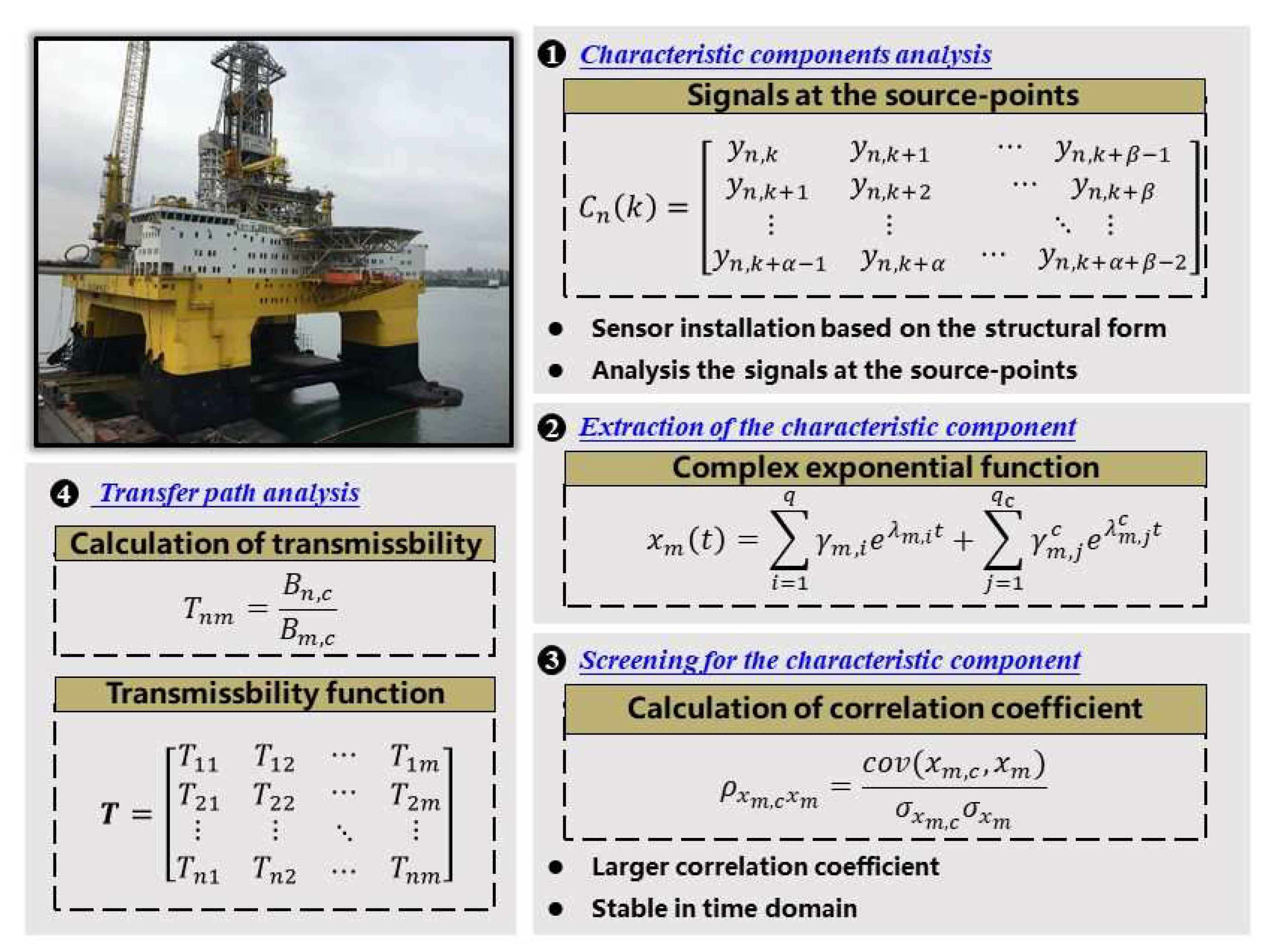
The issues of modeling and the simulation for the transfer path analysis in semi-submersible platforms are shown in Figure 1. The process of the proposed transfer path analysis method can be summarized as four sequential main steps:

• According to the structure form, install sensors at source-points and receiver-points. Then, measure the acceleration signals of each point when the system is in operation. Then, analyze the signals from the source-points by using Equations (6) and (7) to obtain the vibration of frequencies with time and to determine the characteristic components.
• By defining a Hankel matrix as Equation (12), decompose the signals from the receiver-points. In addition, by calculating the frequency of each component via Equation (15), extract the components close frequencies close to the frequency of the characteristic component.
• Calculate the relevance using Equations (16)–(19) and judge the stability of the extracted component to remove the pseudo components and obtain the real stable characteristic component. Quantify the extraction error and ensure the accuracy of extraction by using Equation (21). If the requirement of error is not satisfied, repeat the extraction steps for the residual signals.
• Repeat the steps above for each measured signal and calculate amplitudes of the extracted characteristic signals. Then, calculate the transmissibility function by Equation (23). Next, calculate the matrix of the transmissibility function via Equation (24), and express the transfer path of the characteristic components in the entire space.

4. Numerical Studies: Energy Transfer Path Model

The purpose of this example is to introduce the proposed method through two numerical cases, a 2-DOF model to simulate a single path problem and a 5-DOF model to simulate a multi-path one. In addition, by comparing the results with the OTPA method, we can study the performance of the proposed method. Considering the damped vibration of a transmission system, we can obtain the vibration differential equation of the system by applying the Newton’s law as:

$$\mathbf{M}\ddot{\mathbf{x}}+\mathbf{C}\dot{\mathbf{x}}+\mathbf{k}\mathbf{x}=\mathbf{F}$$

(25)

where $\mathbf{M}$, $\mathbf{C}$, $\mathbf{k}$, $\mathbf{x}$, and $\mathbf{F}$ represent the matrices of mass, damping, stiffness, displacement, and force, respectively.

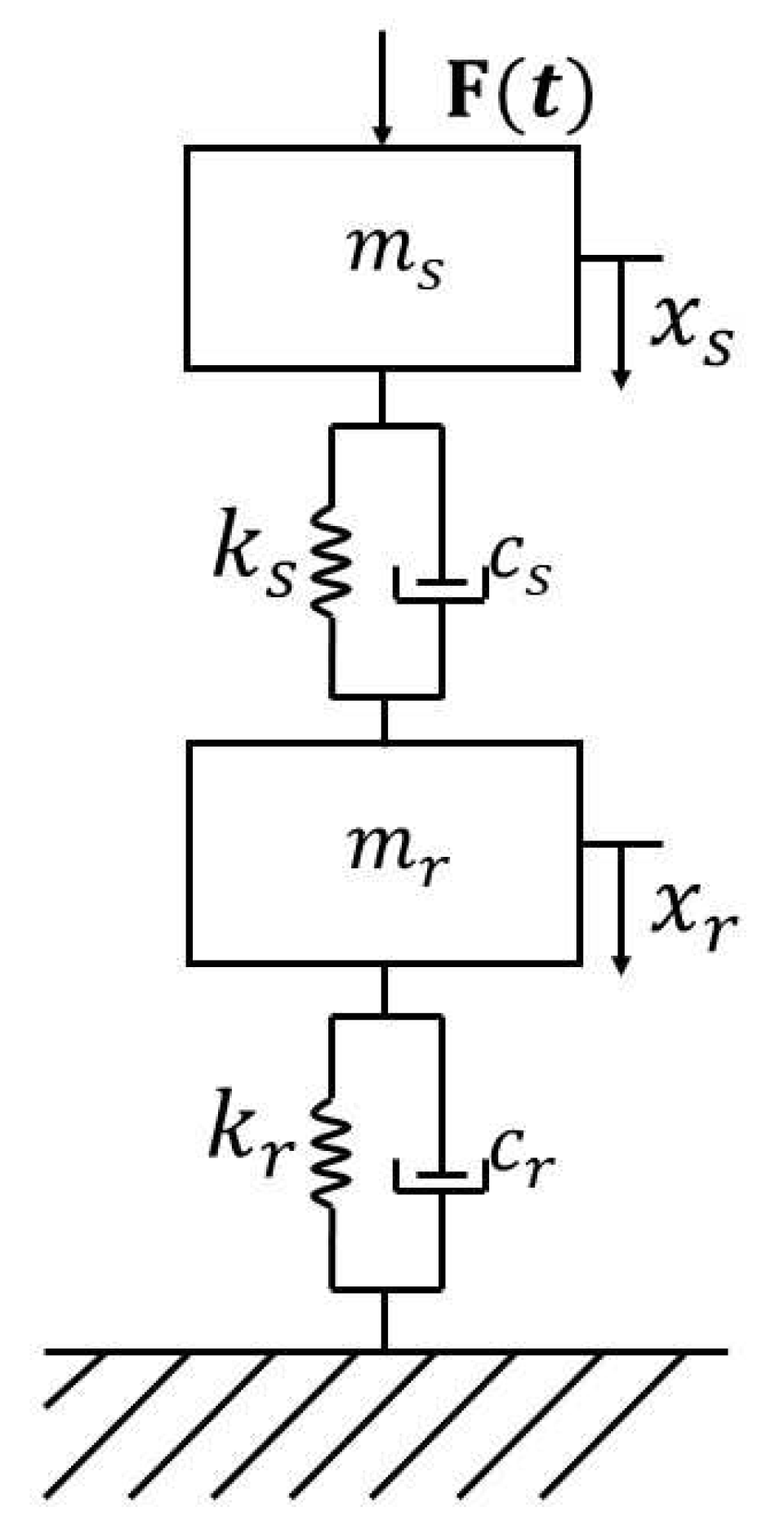
4.1. Case 1: Single-Path Energy Transfer Model

In this case, a 2-DOF model, as shown in Figure 2, was used to simulate the single path transfer model, The parameters of the model were as follows: $m_s=865$ kg, $c_s=340$ N· s/m, $k_s=$30,000 N/m, $m_r=45$ kg, $c_r=65$ N· s/m, $k_r=1000$ N/m, and $F\left(t\right)$ is a pulse load of 200 N. The matrices in Equation (25) are:

$$\mathbf{x}={\left[\begin{array}{cc}{x}_s& x_r\end{array}\right]}^T$$

(26)

$$\mathbf{F}={\left[\begin{array}{cc}F\left(t\right)& 0\end{array}\right]}^T$$

(27)

$$\mathbf{M}=\left[\begin{array}{cc}{m}_s& 0\\ 0& m_r\end{array}\right]$$

(28)

$$\mathbf{C}=\left[\begin{array}{cc}{c}_s& -c_s\\ -c_s& c_s+c_r\end{array}\right]$$

(29)

$$\mathbf{K}=\left[\begin{array}{cc}{k}_s& -k_s\\ -k_s& k_s+k_r\end{array}\right]$$

(30)

The transmissibility functions reflect the relationships between the output and the input. To evaluate the accuracy of the transmissibility functions, we used the output calculated by Equation (25) and the output calculated by the transmissibility functions as a comparison. The specific process is as follows:

• After applying the excitation force on $m_s$, the acceleration response of $m_s$ and $m_r$ can be calculated by Equation (25).
• Implement the Fourier transform on the calculated response of $m_r$, and consider it as the real value.
• Extract the characteristic component of the response of $m_s$ and $m_r$. Then, calculate the amplitudes of the characteristic components to obtain the transmissibility functions. Use the response of $m_s$ to multiply the transmissibility functions and implement the Fourier transform on the obtained response. Consider the result to be the calculated value.
• Compare the real value and the calculated value, and the accuracy of the proposed method can be shown.

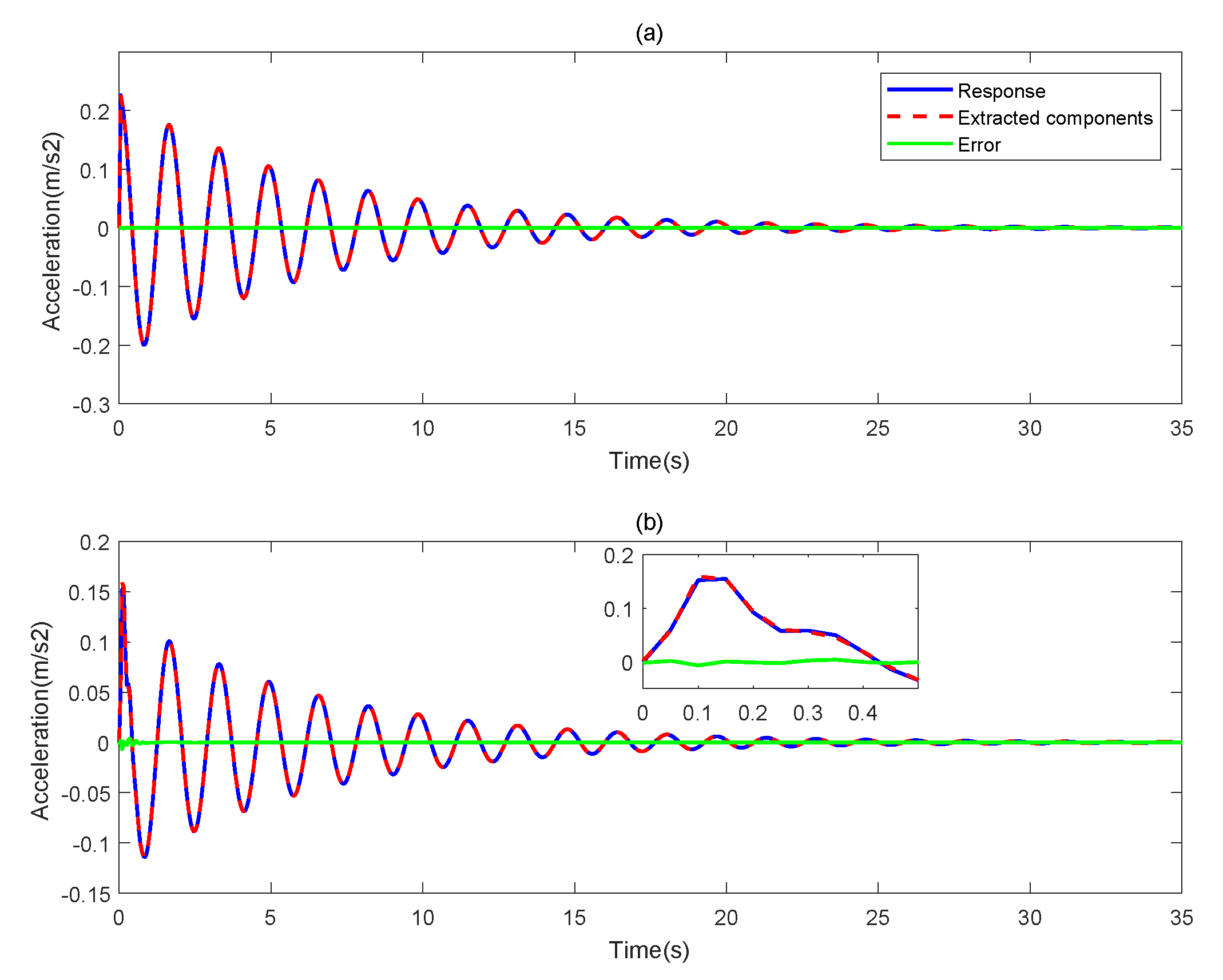
After removing the force, the system will vibrate. First, by calculating Equation (25), the responses of $m_r$ and $m_s$ can be obtained, as shown by the blue line in Figure 3. By implementing Fourier transform on the response of $m_r$, the result is shown as the blue line in Figure 4, which can be considered accurate. By using the complex exponential decomposition, the characteristic component can be obtained. Through the analysis of eigenvalues, the natural frequencies of the 2-DOF are 0.6121 Hz and 5.141 Hz. Under the excitation of $F\left(t\right)$, the responses of $m_s$ and $m_r$ only have one frequency, 0.6107 Hz. This means only the first-order frequency is excited. The result is consistent with the results by solving eigenvalues. In addition, the response and the extracted component should be equal in theory. The characteristic components that are extracted by the proposed method are shown as the red line in Figure 3. We can see the error between the response and the extracted component are very small and the two lines are almost consistent.

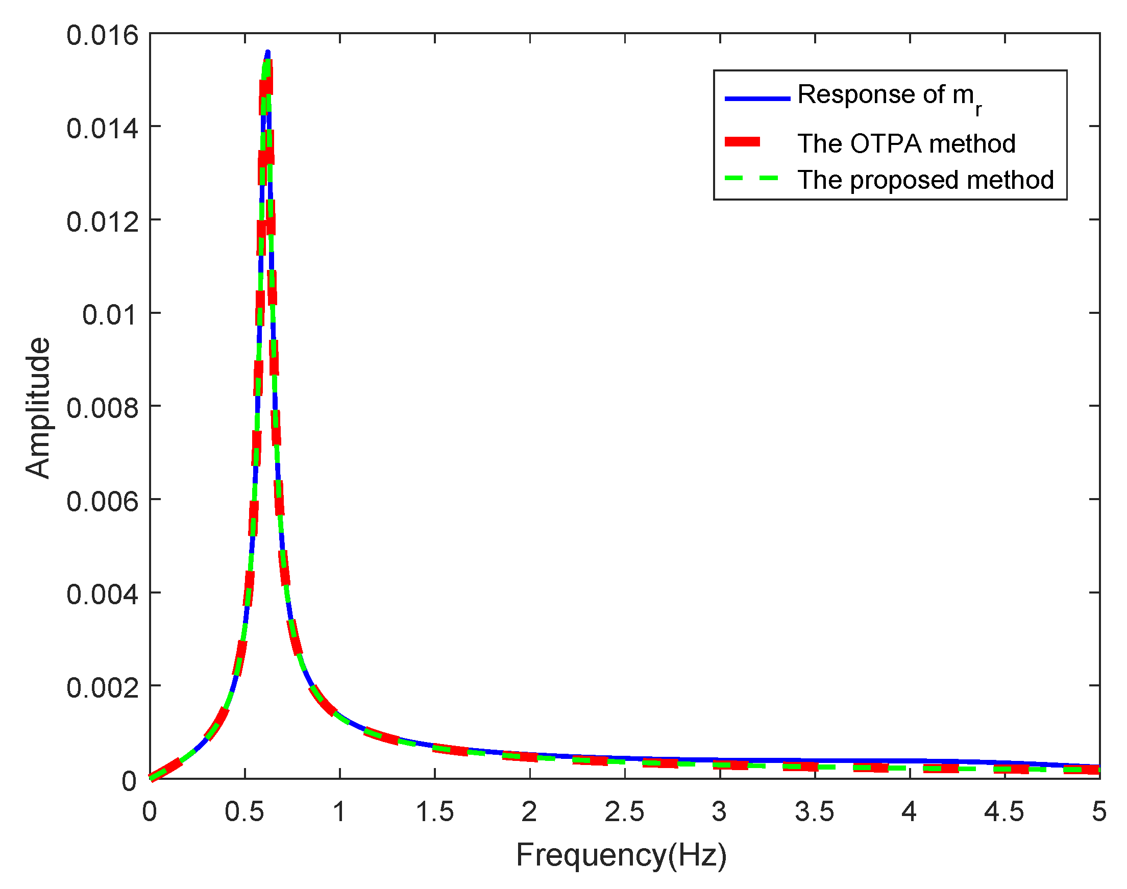
After the extraction, only one component is obtained, and the amplitude, which equals 0.0272, can be calculated by Equation (20). The same equation for the response of $m_r$ can be used to calculate the amplitude of the characteristic component, which is 0.0156. Then, by Equation (23), the transmissibility function, which equals 0.5737, can be obtained. By using the response of $m_s$ to multiply the transmissibility function, the result in the frequency domain is plotted in Figure 4 as the green line. In addition, we can calculate the result of the OTPA method to make a comparison. In the OTPA method, the transfer functions are first calculated. Here, the transfer function is calculated by using the state–space model, which has been proven to be an efficient and accurate method [20,21]. After obtaining the ratio of the transfer functions, we can use it to multiply the response of $m_s$, and the result by Fourier transform is plotted as the red line in Figure 4. As shown in Figure 4, the results obtained by the three methods are consistent, which verifies the validity and analytical accuracy of the proposed method.

4.2. Case 2: Multi-Path Energy Transfer Model

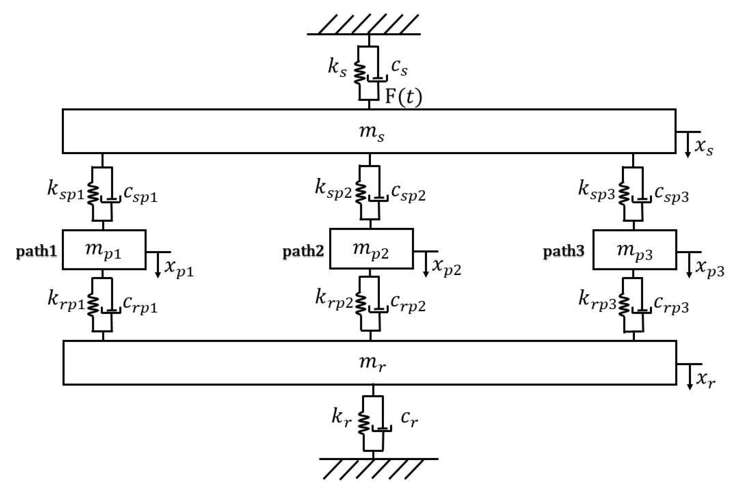
In this case, a 5-DOF model, as shown in Figure 5, was used to simulate the multi-path transfer model, and the energy of the vibration source was transmitted to the receiving-point through the three paths. $m_s$ and $m_r$ are the mass of the vibration source-point and the receiving-point. $m_{p1}$, $m_{p2}$, and $m_{p3}$ are the mass of the suspension in Paths 1–3, respectively. In addition, k is the stiffness, $k_s=500$ N/m, $m_r=0.5$ kg, $c_r=1$ N· s/m, $k_r=1000$ N/m, $m_{p1}=0.4$ kg, $m_{p2}=0.5$ kg, $m_{p3}=0.6$ kg, $c_{sp1}=c_{rp1}=6$ N·s/m, $c_{sp2}=c_{rp2}=4$ N·s/m, $c_{sp3}=c_{rp3}=8$ N·s/m, $k_{sp1}=k_{rp1}=800$ N/m, $k_{sp2}=k_{rp2}=600$ N/m, $k_{sp3}=k_{rp3}=400$ N/m, and $F\left(t\right)$ is a pulse load of 200 N. For the multi-path transfer model, the matrices in Equation (25) are:

$$\mathbf{x}={\left[\begin{array}{ccccc}{x}_s& x_{p1}& x_{p2}& x_{p3}& x_r\end{array}\right]}^T$$

(31)

$$\mathbf{F}={\left[\begin{array}{ccccc}F\left(t\right)& 0& 0& 0& 0\end{array}\right]}^T$$

(32)

$$\mathbf{M}=\left[\begin{array}{ccccc}{m}_s& 0& 0& 0& 0\\ 0& m_{p1}& 0& 0& 0\\ 0& 0& m_{p2}& 0& 0\\ 0& 0& 0& m_{p3}& 0\\ 0& 0& 0& 0& m_r\end{array}\right]$$

(33)

$$\mathbf{C}=\left[\begin{array}{ccccc}{c}_s+c_{sp1}+c_{sp2}+c_{sp3}& -c_{sp1}& -c_{sp2}& -c_{sp3}& 0\\ -c_{sp1}& c_{sp1}+c_{rp1}& 0& 0& -c_{rp1}\\ -c_{sp2}& 0& c_{sp2}+c_{rp2}& 0& -c_{rp2}\\ -c_{sp3}& 0& 0& c_{sp3}+c_{rp3}& -c_{rp3}\\ 0& -c_{rp1}& -c_{rp2}& -c_{rp3}& c_r+c_{rp1}+c_{rp2}+c_{rp3}\end{array}\right]$$

(34)

$$\mathbf{K}=\left[\begin{array}{ccccc}{k}_s+k_{sp1}+k_{sp2}+k_{sp3}& -k_{sp1}& -k_{sp2}& -k_{sp3}& 0\\ -k_{sp1}& k_{sp1}+k_{rp1}& 0& 0& -k_{rp1}\\ -k_{sp2}& 0& k_{sp2}+k_{rp2}& 0& -k_{rp2}\\ -k_{sp3}& 0& 0& k_{sp3}+k_{rp3}& -k_{rp3}\\ 0& -k_{rp1}& -k_{rp2}& -k_{rp3}& k_r+k_{rp1}+k_{rp2}+k_{rp3}\end{array}\right]$$

(35)

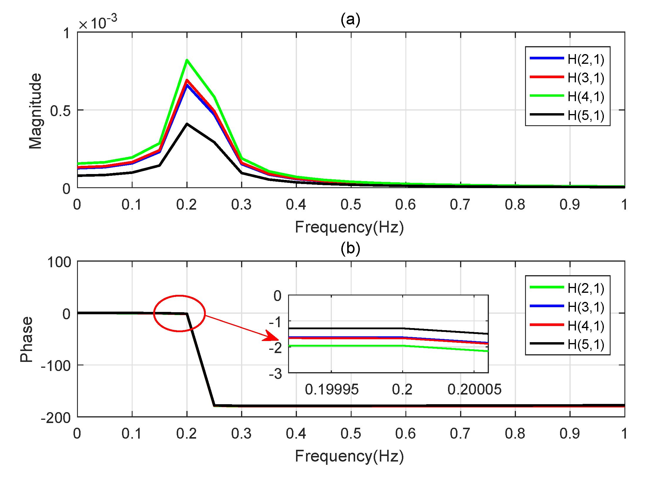
Before using the proposed method, we first use the OTPA method to obtain a standard result. By using the OTPA method, the first step is to calculate the transfer functions. As shown in Figure 6, the transfer functions are calculated by using the method in [20]. Figure 6a,b corresponds to the amplitude–frequency diagram and the phase–frequency diagram of the calculated transfer functions, respectively. In Figure 6, the blue line represents the transfer function between $m_{p1}$ and $m_s$, the red line represents the transfer function between $m_{p2}$ and $m_s$, the green line represents the transfer function between $m_{p3}$ and $m_s$, and the black line represents the transfer function between $m_r$ and $m_s$. After obtaining the transfer functions, the second step is to calculate the transmissibility function. By implementing the Fourier transform to each transfer function and calculating the ratio of the amplitudes, the results of transmissibility function are shown in

Table 1. The results of transmissibility functions under three types of force, and the traditional OTPA result.

		Path 1	Path 2	Path 3
The OTPA method		0.6213	0.5932	0.5005
The proposed method	Pulse load: 200 N	0.6223	0.5938	0.5008
	$F\left(t\right)=100\sin (2\pi \times 40t+\pi /4)$	0.6215	0.5936	0.5008
	10% Gaussian white noise	0.6217	0.5935	0.5005

. In addition, they can also be expressed as the dark blue bar in Figure 7.

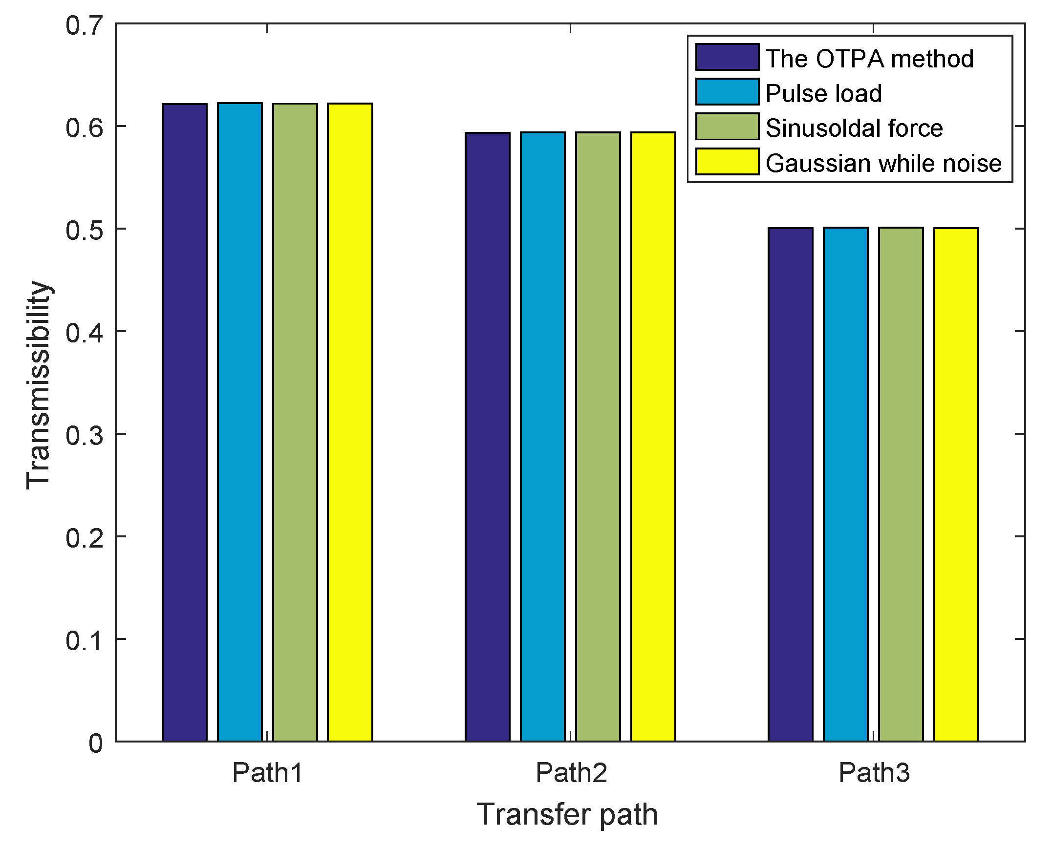
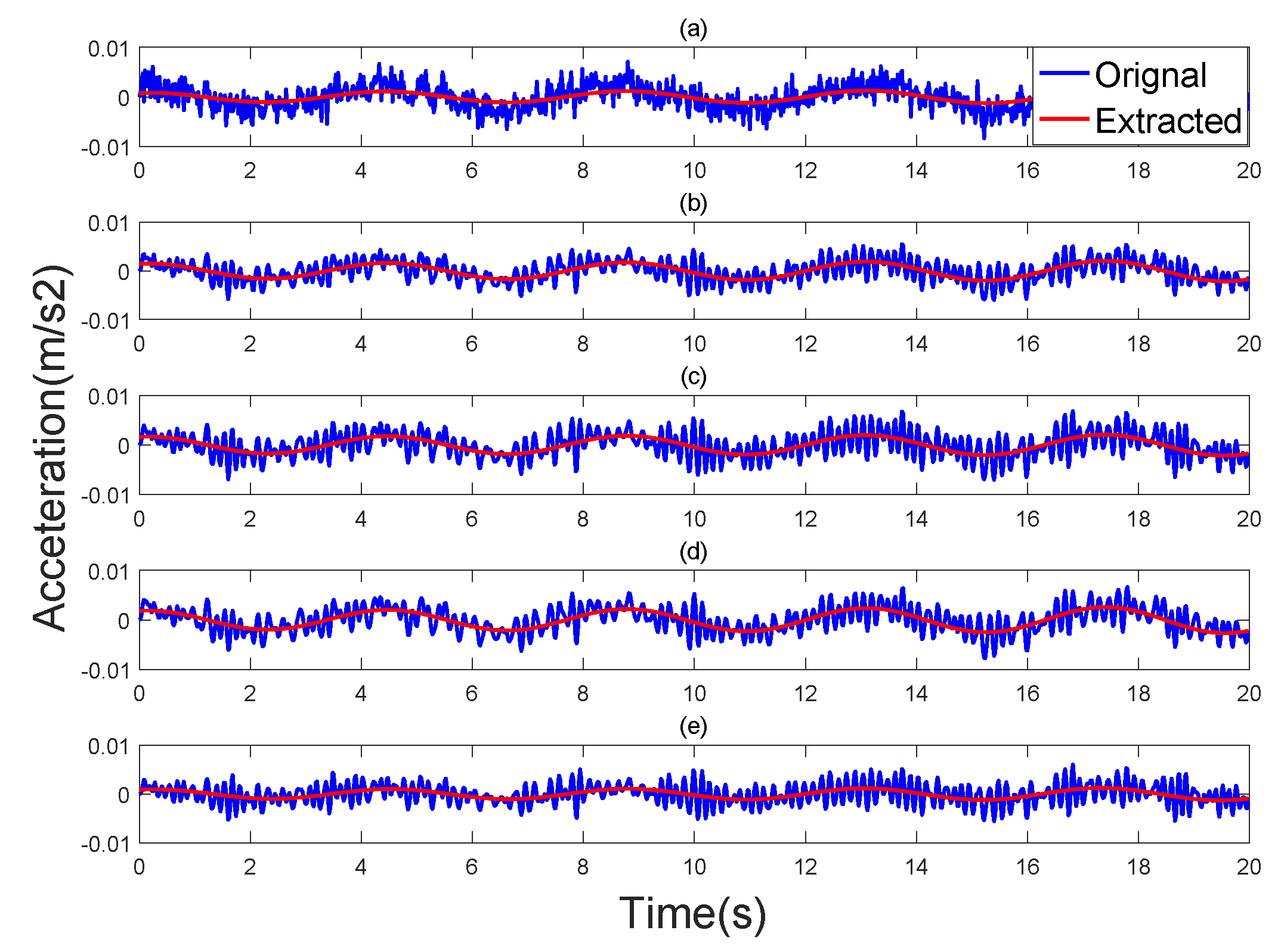
In implementing the proposed method, the excitation force is set to be a pulse load of 200 N. Substituting the parameters into Equation (25), the response of the source-point and receiver-points can be obtained. The calculated responses of $m_s$, $m_{p1}$, $m_{p2}$, $m_{p3}$, and $m_r$ are shown with the blue line in Figure 8. By using the proposed method, the extracted components in the time domain are also plotted with the red line in Figure 8. After extraction, by calculating the amplitudes of the extracted component, the transmissibility function can be obtained, which are shown in Table 1. The transmissibility function is determined by the essential characteristics of the system and will not change. Therefore, in this case, two other kinds of excitation forces, i.e., a sinusoidal force $F\left(t\right)=100sin(2\pi \times 40t+\pi /4)$ and a 10% Gaussian white noise excitation, are used to calculate the transmissibility functions. The results of transmissibility functions are also shown in Table 1 and the results are plotted in Figure 7.

From the result, we can see that, since the stiffness and the damping parameters of the three paths are different, the three paths have different contributions to the receiving end when transmitting the vibration energy, where in the contribution of Path 1 is the largest. In addition, in the numerical model, OTPA has been proven to have a high precision [6]. Therefore, OTPA is used to obtain reference results to compare with the proposed method. In Table 1, we can see that results from the proposed method are almost the same as those from OTPA. At the same time, under different types of force, the results obtained by using the proposed method are almost consistent, with very little error. This can also prove that, when the input force and the transfer function are unknown, the transmissibility functions can be obtained with only the output response by using the proposed method.

5. Experimental Study

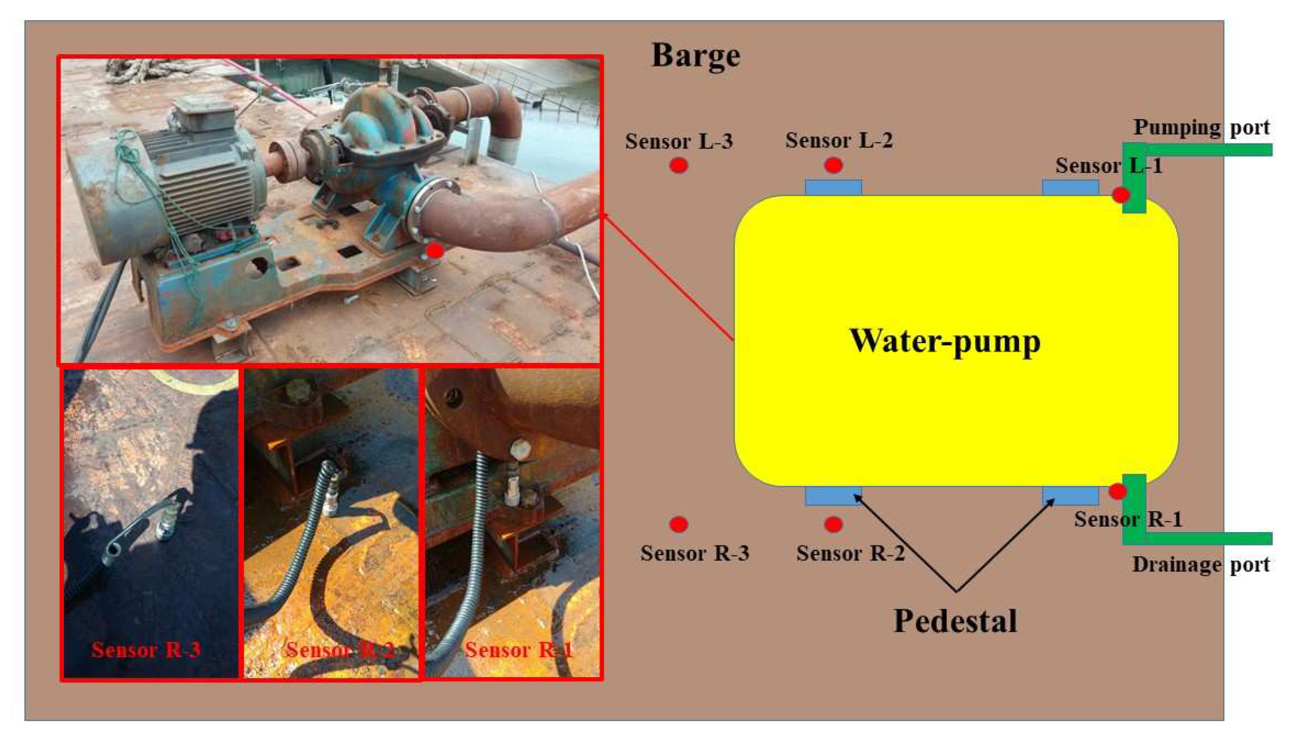
To further study the effectiveness of the proposed method, an experimental study of the vibration transfer path was conducted. To simulate the marine environment of an semisubmersible platform, the experiment was carried out on a barge berthed in a deep-water pier that is located in Yantai, Shandong Province of China. The size of the barge was 60 m × 35 m × 6 m. To simulate the excitation signal of the vibration source, a 20 kW water-pump was used to provide the excitation force in the experiment, and the vibration was generated by pumping and draining water. The supporting structures of the water-pump were simulated by two sets of symmetrical steel frames. The size of the frame was 2330 mm × 90 mm × 200 mm. The steel frame was welded on the barge, and the distance between the two sets of steel frames was 550 mm. The water-pump straddled the two sets of steel frames. Six acceleration sensors were installed on the structure to measure the dynamic response at different locations of the structure. The layout of the experiment is shown in Figure 9. The sensors were installed on the left and right sides of the pedestal, with three sensors on each side. Two sensors were at the water-pump, two sensors were near the pedestal, and two were at a distance of 50 cm. After the pump was running smoothly, synchronous sampling was performed with a 5120 Hz sampling frequency.

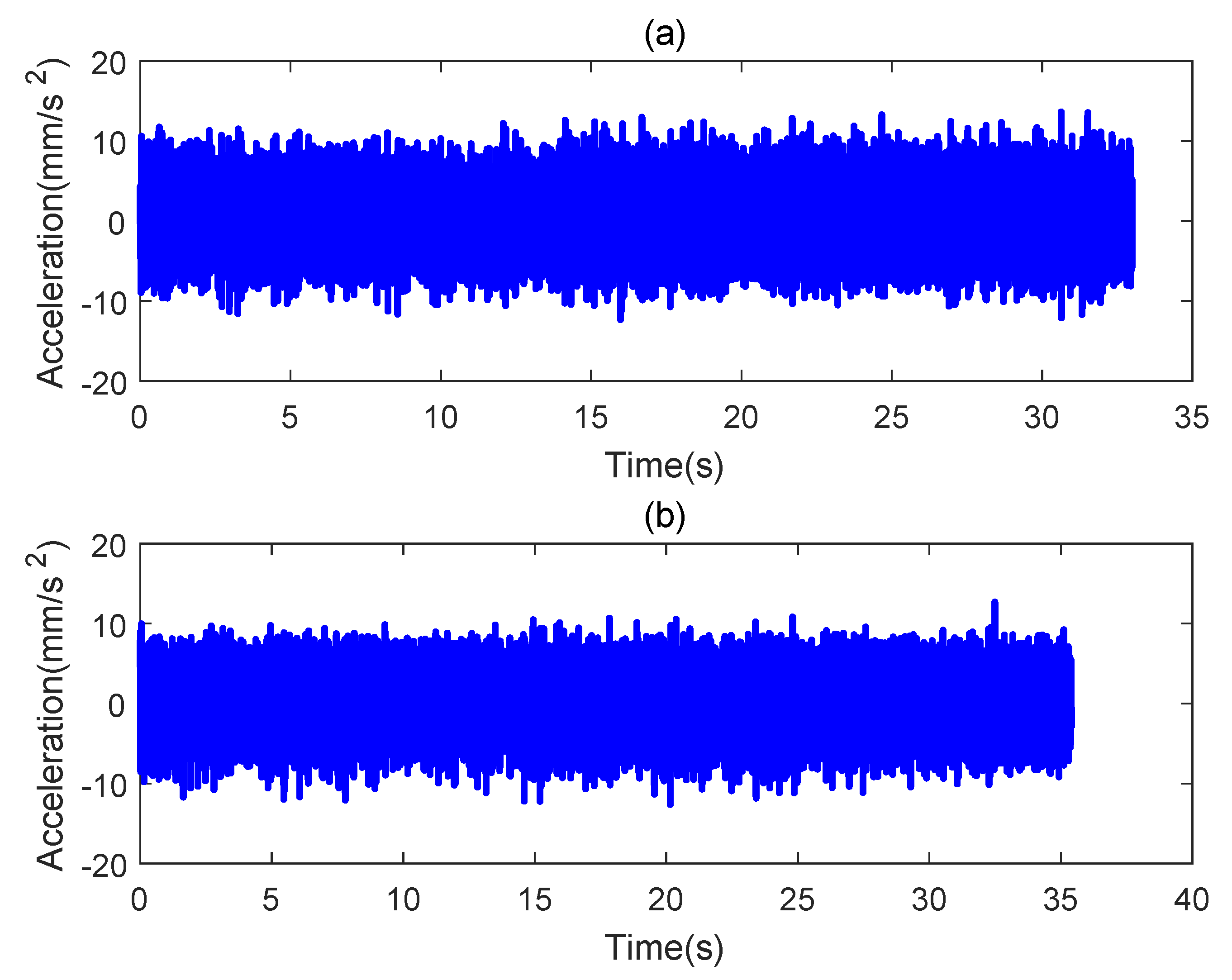
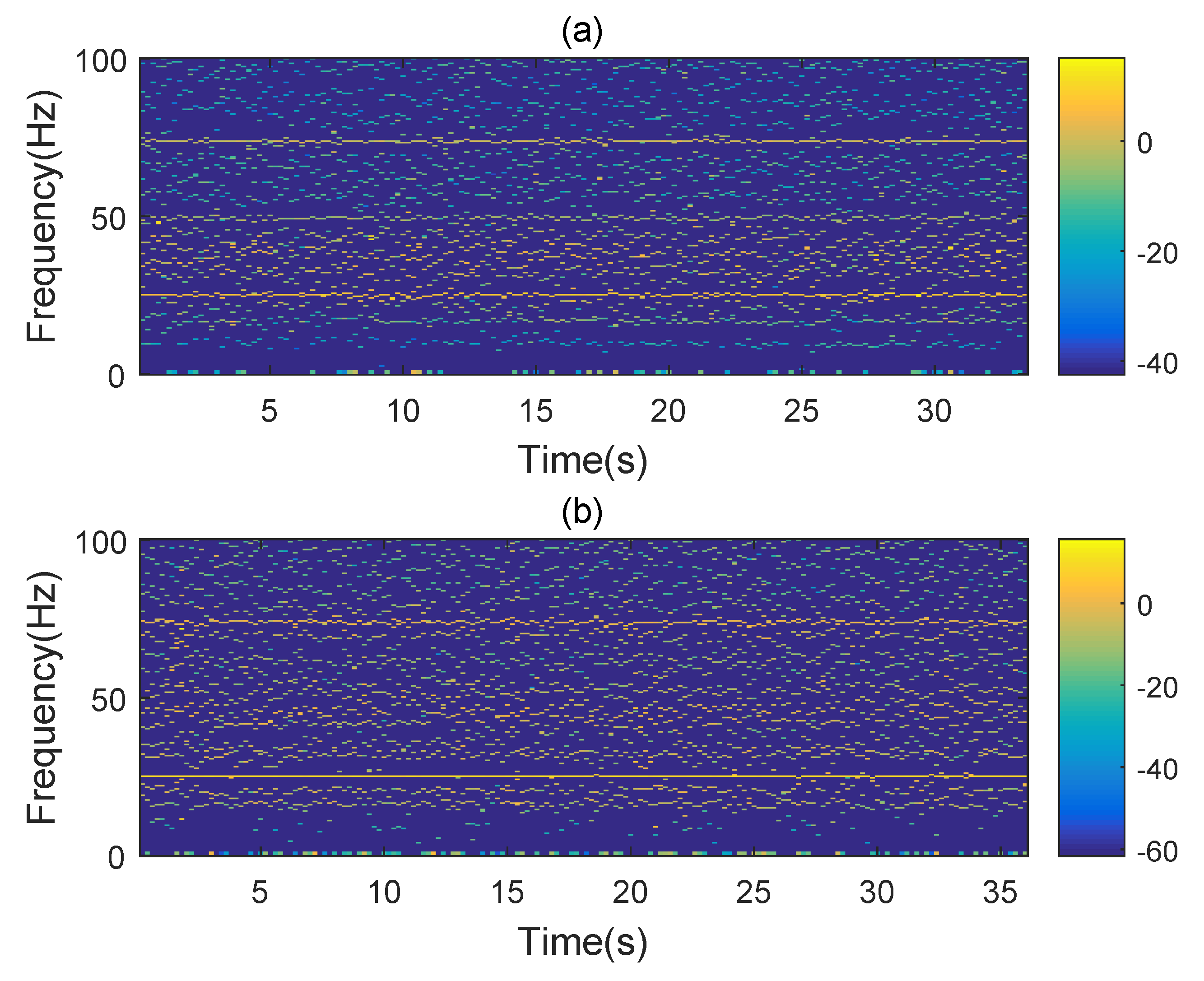
In the proposed method, the first step is to determine the characteristic components of the two sources. The waveform of two signals that is measured from “Sensor L-1” and “Sensor R-1” can be seen in Figure 10a and Figure 11b. In addition, by implementing Equations (6) and (7), the vibrations of frequencies are shown in Figure 11. As shown in Figure 11, at both sides of the water-pump, the vibration at 24 Hz is the strongest. Therefore, the component with 24 Hz is considered to be a characteristic component. As the left side and the right side are treated similarly, here we take the left side as an example for analysis. After the determination of the characteristic component, we studied the transfer of the characteristic component.

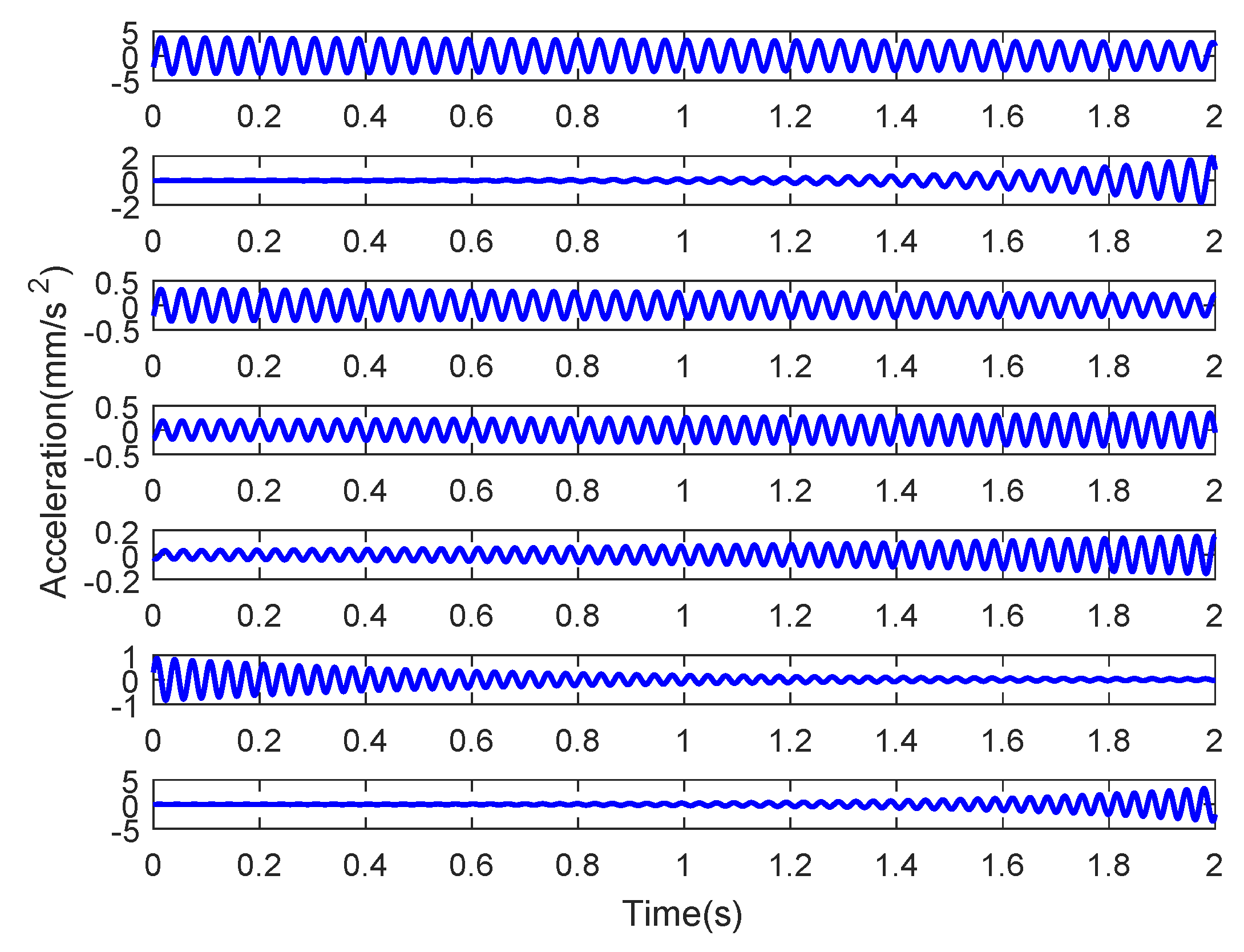
First, we analyzed the signal that was measured from “Sensor L-1”. By implementing the signal decomposition, seven signals whose frequencies are near 24 Hz are extracted as shown in Figure 12. However, which is the characteristic component cannot be determined only from the signal in the time domain. Therefore, a correlation step should be implemented. Calculate the correlation coefficients of each component separately; the correlation results are 0.9300, 0.1115, 0.02737, 0.0204, 0.00496, 0.0203, and 0.0843. From the values, we can see that the correlation of the first component is the biggest, and this is considered the characteristic component. However, in fact, we cannot guarantee that the principle component is extracted clean. Therefore, the extraction process is repeated until the screening criteria are satisfied and the screening criterion is set to be $\delta =1\times {10}^{-6}$.

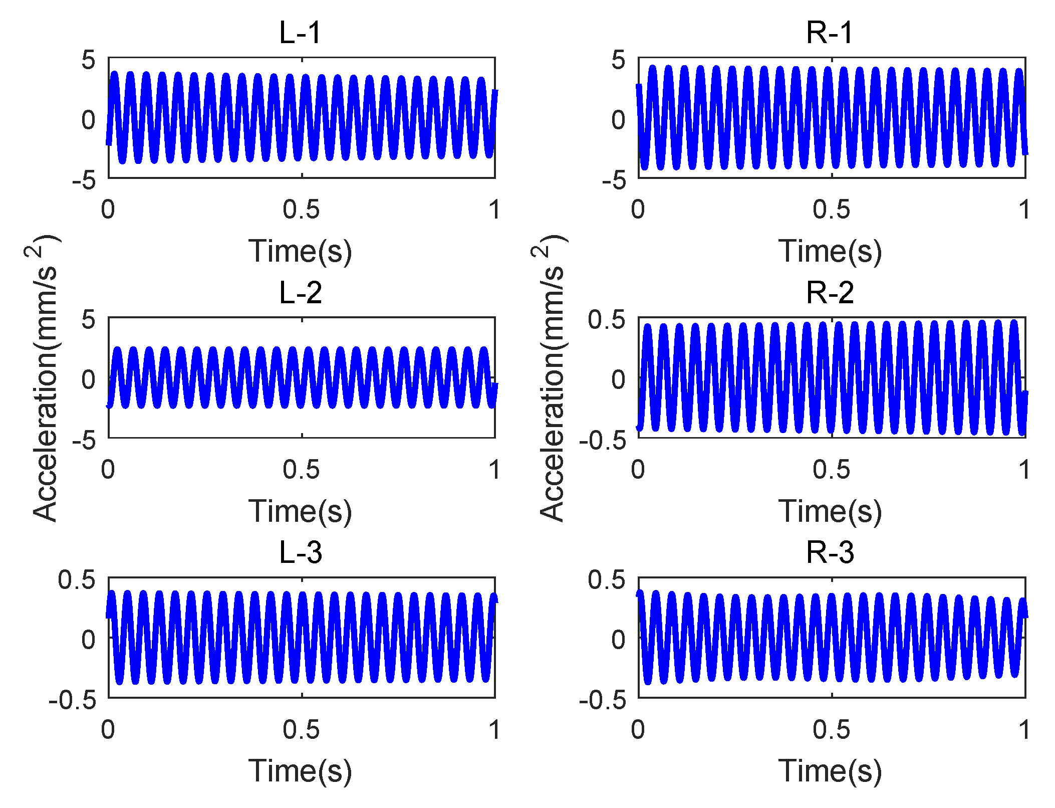
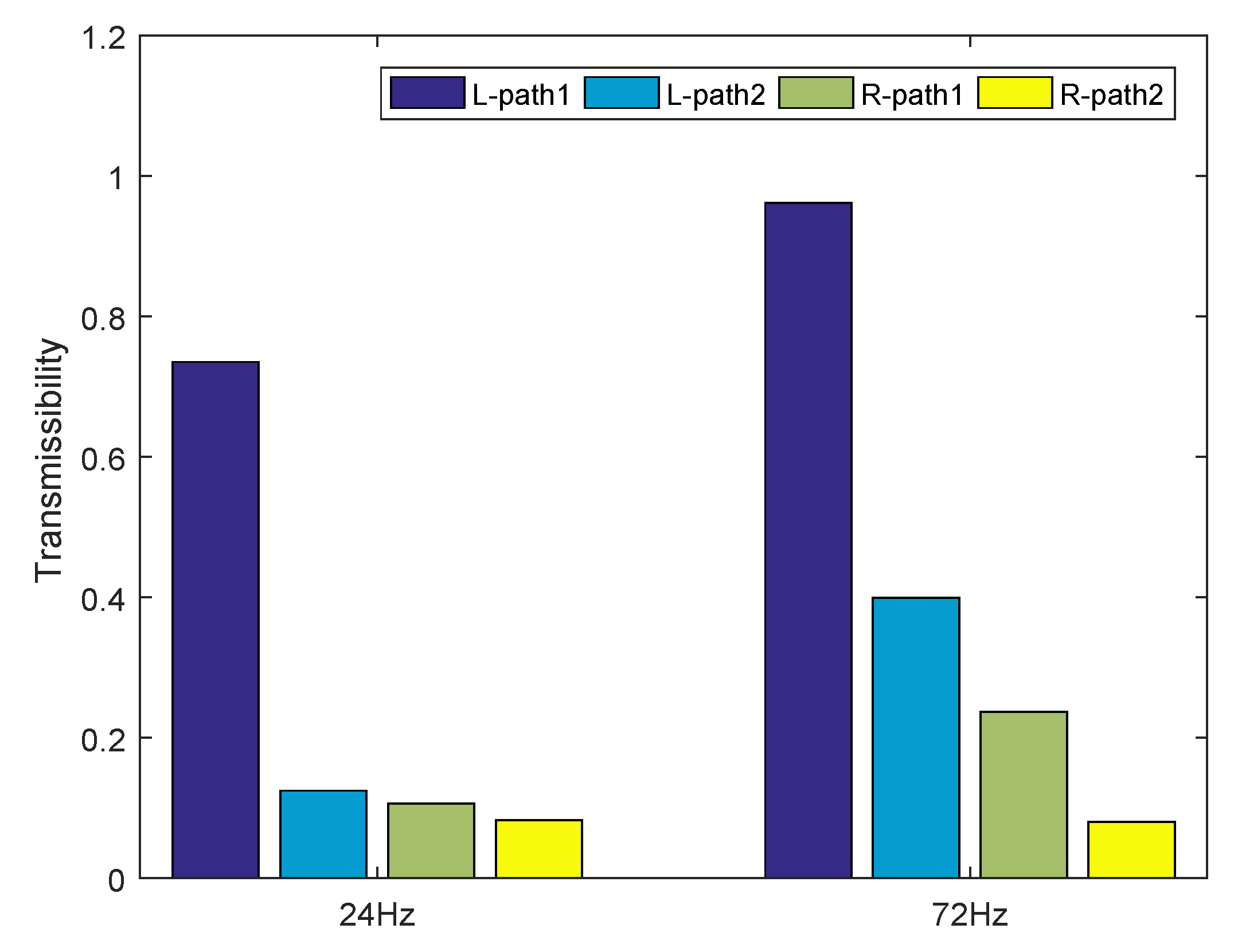
After extraction, the characteristic components in the six sensors can be obtained, as shown in Figure 13. The transmissibility function, defined as the ratio of the amplitude of characteristic components, can be calculated as: $T_{L21}=0.7351$ and $T_{L31}=0.1246$. By repeating the steps, we can also obtain the transmissibility functions of the right side, and the results are: $T_{R21}=0.7351$ and $T_{R31}=0.1246$. The values are shown in Figure 14. Similarly, the transmissibility functions of the characteristic component with 72 Hz are calculated, as shown in

Table 2. The results of transmissibility functions of the left side and the right side.

Characteristic Frequencies	Left: ${\mathit{T}}_{\mathit{L}21}$	Left: ${\mathit{T}}_{\mathit{L}31}$	Right: ${\mathit{T}}_{\mathit{R}21}$	Right: ${\mathit{T}}_{\mathit{R}31}$
24 Hz	0.7351	0.1246	0.1064	0.0824
72 Hz	0.9614	0.3992	0.2369	0.0803

. Furthermore, in Figure 11, we can see that there are other obvious energy components that are concentrated in 72 Hz. In addition, the results obtained by using the proposed method are also shown in Figure 14. From the results, we can see that, in this experiment, the most important energy transfer path is concentrated on the left side from “Sensor L-1” to “Sensor L-2”. In addition, by comparing the transmissibility functions of components at 24 and 72 Hz, we can see the change of transmissibility functions are consistent for components of different frequencies. Thus, by using the proposed method, the vibration transmissions are quantified only by the output responses, and this would also help us to deal with the vibration isolation measures in engineering.

6. Field Test Study: The Energy Transmission in a DP Cabin

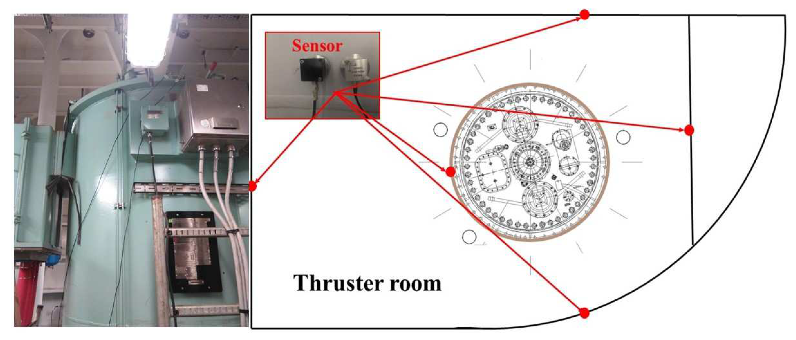
A field text was also performed on a deep-sea semi-submersible platform during its sea trial. The sea trial position was located in the dynamic positioning (DP) cabin of the platform, which is 13.2 m long, 7.83 m wide, and 5.8 × 2 m high. Fove accelerometers were installed to test the response of each bulkhead. As shown in Figure 15, the sensors were located at the propeller foundation and at the surrounding bulkheads. During the test, the motor speed was set to 680 rpm and 620 rpm, respectively. The sampling frequency was set to 20,000 Hz.

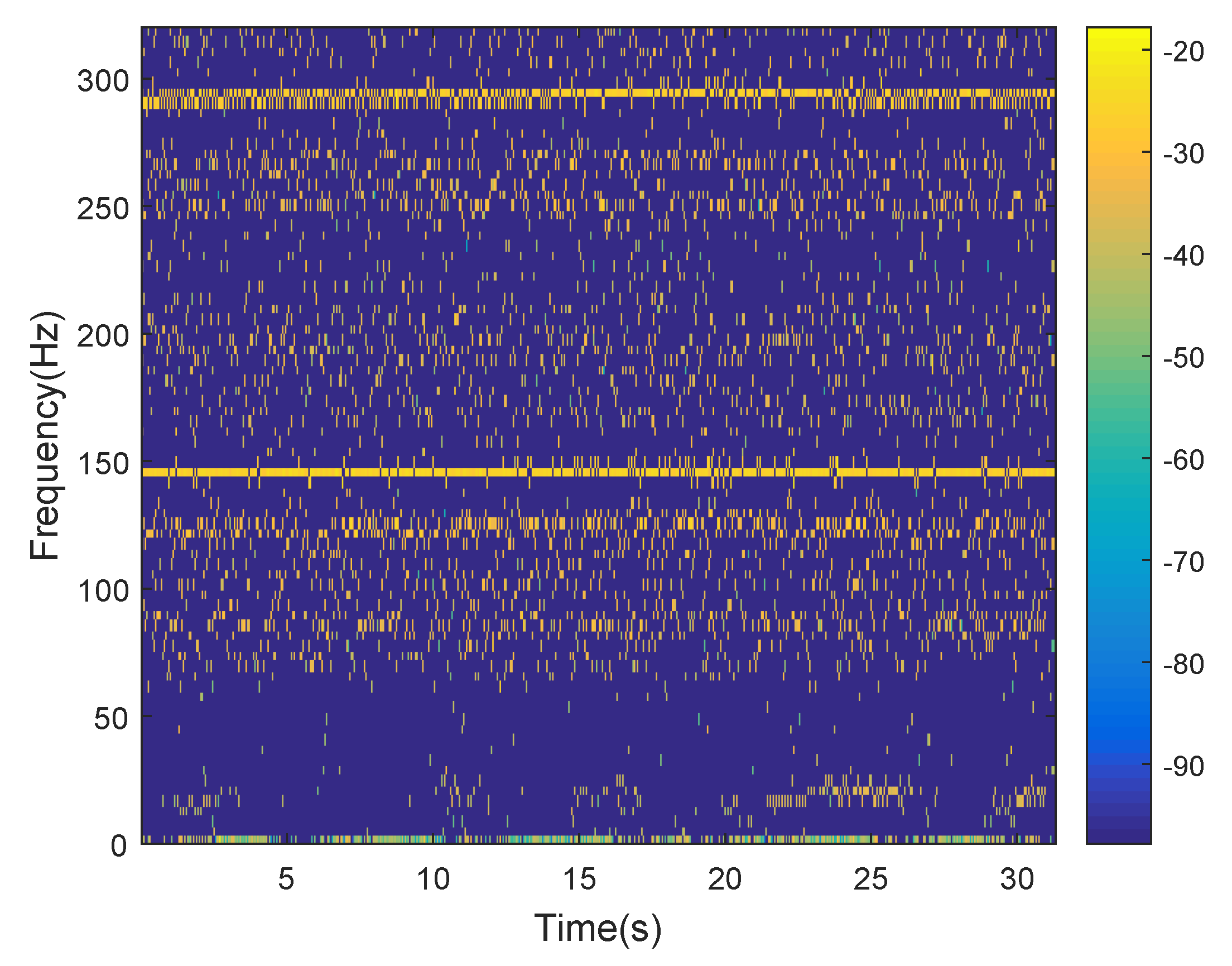
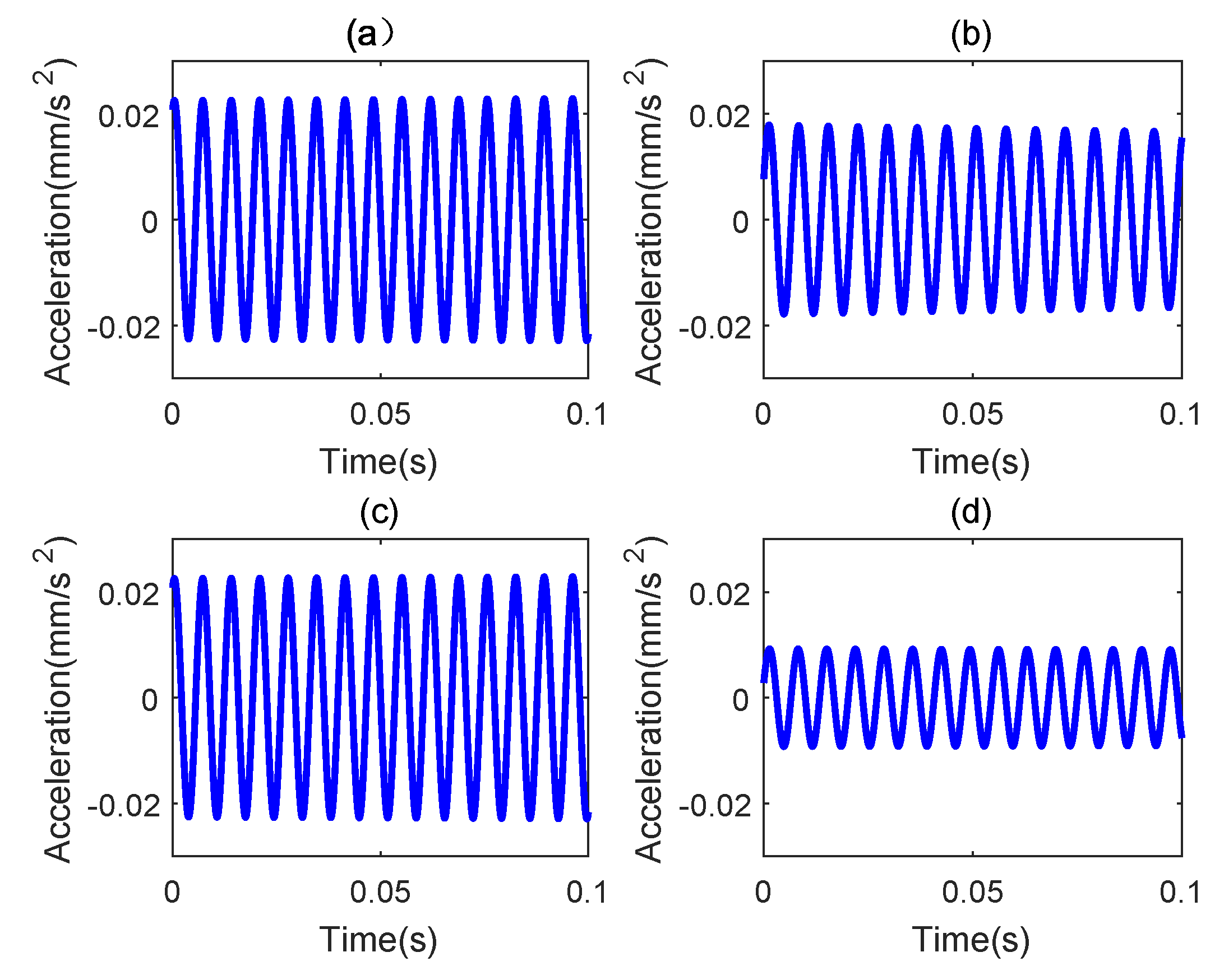
First, we analyzed the situation when the propeller motor speed was 680 rmp. Figure 16 shows the identified characteristic components of the signal measured from the sensor at the foundation. From the result, we can see that the characteristic components are near 146 Hz and 292 Hz. After determination, we analyzed the characteristic components of the signal at each bulkhead. Through signal decomposition and a correlation analysis, the components at 146 Hz extracted from the receiver-sensors are shown in Figure 17. The same extraction analysis was performed at 292 Hz. After extraction, the amplitudes can be calculated and the transmissibility functions can be obtained. Next, the condition with a propeller speed of 620 rmp was analyzed. We could find that the characteristic components are at 135 Hz and 270 Hz. By extracting and calculating, the transmissibility functions are shown in

Table 3. The results of transmissibility functions of the four directions.

	Starboard	Stern	Port	Bow
620 rmp (135 Hz)	0.3846	0.3670	0.1591	0.0812
620 rmp (270 Hz)	0.4630	0.3722	0.1279	0.0236
680 rmp (146 Hz)	0.3444	0.2931	0.1182	0.0392
680 rmp (292 Hz)	0.4406	0.3281	0.1156	0.0781

.

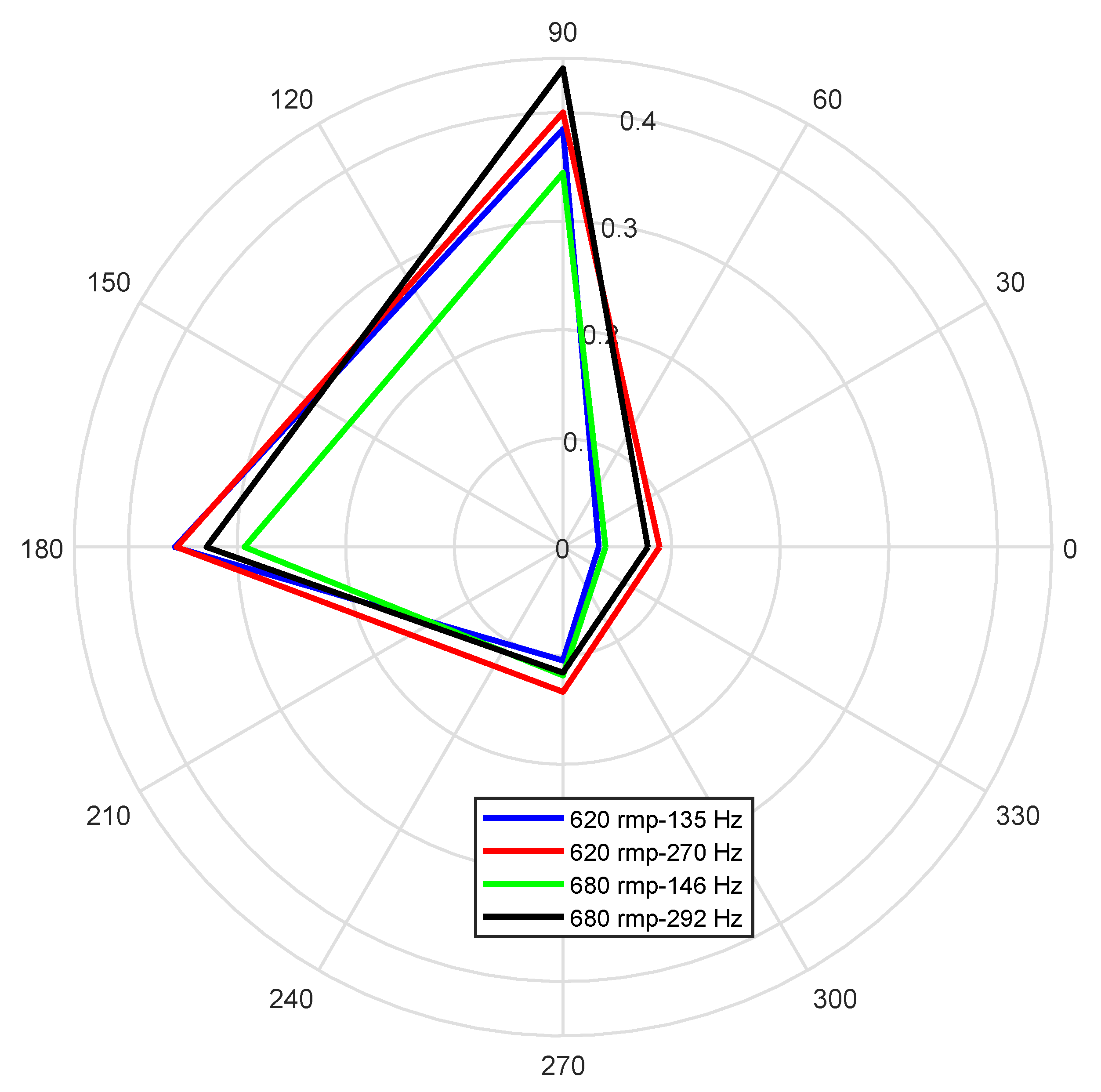
To represent the results of transmissibility functions more intuitively, the radar graph was introduced, as shown in Figure 18. The blue line and the red line represent the transmissibility functions of the components of 135 Hz and 270 Hz, respectively, under 620 rmp. The green line and the black line correspond to the components of 146 Hz and 292 Hz, respectively, under 680 rmp. In Figure 18, we can see the transmission rules of the characteristic components at different speeds and of different frequencies are basically the same. The largest amount of energy is transmitted to the center axis of the structure, and a part of the larger energy is transmitted to the stern of the structure. The starboard and bow part are corresponding to the outer structure of the hull. Since the outer portion of the structure is used to resist external shocks, etc., the design strength is large, thus the vibration transmission there is weaker than in other parts. This is also consistent with the structural design of the hull.

7. Conclusions

Based on state–space model and the concept of transmissibility function, a new TPA method is proposed to study the energy transfer path of the characteristic component in semi-submersible platforms. The proposed method contains four steps: (1) analyzing the vibration of frequencies on the source-points to determine the characteristic components; (2) introducing a state–space model to decompose the measured signals; (3) using the correlation function to extract the characteristic components based on the $L_2$-norm standard; and (4) calculating the ratio of the amplitudes to obtain the transmissibility functions. By using the proposed method, the transfer path analysis in complex offshore platforms can be analyzed with the output responses. In addition, the frequency leakage can be overcome and the accuracy can be improved.

Three examples are presented in the paper. In the first example, two models, a 2-DOF model and a 5-DOF model, were used to prove the correctness of the concept of transmissibility functions. By comparing the proposed method with the traditional method, it is shown that the results from the proposed method by using the response only are accurate. The second example used the data from an experiment implemented on a barge. The results show that the proposed method can effectively analyze the transfer path of characteristic components. Finally, sea trial data from a DP cabin were used. From the analysis results, we can see that the new method can effectively identify the transfer path of a characteristic component in offshore platforms. It can be used to evaluate the transfer path quantitatively, and has potential value of application in engineering.

References

- Li, Z.X.; Peng, Z. A new nonlinear blind source separation method with chaos indicators for decoupling diagnosis of hybrid failures: A marine propulsion gearbox case with a large speed variation. Chaos Solitons Fractals 2016, 89, 27–39. [Google Scholar] [CrossRef]
- Chen, M.F.; Ye, T.G.; Zhang, J.H.; Jin, G.Y.; Zhang, Y.T.; Xue, Y.Q.; Ma, X.L.; Liu, Z.G. Isogeometric three-dimensional vibration of variable thickness parallelogram plates with in-plane functionally graded porous materials. Int. J. Mech. Sci. 2019, 169, 105304. [Google Scholar] [CrossRef]
- Plunt, J. Finding and fixing vehicle NVH problems with transfer path analysis. Sound Vib. 2005, 39, 12–16. [Google Scholar]
- Thite, A.N.; Thompson, D.J. The quantification of structure-borne transmission paths by inverse methods. Part 1: Improved singular value rejection methods. J. Sound Vibr. 2003, 264, 411–431. [Google Scholar] [CrossRef]
- Oriol, G.; Carlos, G.; Jordi, J.; Pere, A. Experimental validation of the direct transmissibility approach to classical transfer path analysis on a mechanical setup. Mech. Syst. Signal Proc. 2013, 37, 353–369. [Google Scholar]
- Sitter, G.D.; Devriendt, C.; Guillaume, P.; Pruyt, E. Operational transfer path analysis. Mech. Syst. Signal Proc. 2010, 24, 416–431. [Google Scholar] [CrossRef]
- Kim, B.-L.; Jung, J.-Y.; Oh, I.-K. Modified transfer path analysis considering transmissibility functions for accurate estimation of vibration source. J. Sound Vibr. 2017, 398, 70–83. [Google Scholar] [CrossRef]
- Stevens, K. Force identification problems—An overview. In Proceedings of the 1987 SEM Spring Conference on Experimental Mechanics, Houston, TX, USA, 14–19 June 1987. [Google Scholar]
- Dobson, B.J.; Rider, E. A review of the indirect calculation of excitation forces from measured structural response data. Proc. Inst. Mech. Eng. Part C J. Eng. Mech. Eng. Sci. 1990, 204, 69–75. [Google Scholar] [CrossRef]
- Gajdatsy, P.; Janssens, K.; Desmet, W.; de Auweraer, H.V. Application of the transmissibility concept in transfer path analysis. Mech. Syst. Signal Proc. 2010, 24, 1963–1976. [Google Scholar] [CrossRef]
- Ribeiro, A.M.R.; Silva, J.M.M.; Maia, N.M.M. On The Generalisation Of The Transmissibility Concept. Mech. Syst. Signal Proc. 2000, 14, 29–35. [Google Scholar] [CrossRef]
- Noumura, K.; Yoshida, J. Method of transfer path analysis for vehicle interior sound with no excitation experiment. In Proceedings of the 31st World Automotive Congress, Yokohama, Japan, 22–27 October 2006. [Google Scholar]
- Gajdasty, P.; Janssens, K.; Gielen, L.; Mas, P. Critical assessment of operational path analysis: Effect of coupling between path inputs. J. Acoust. Soc. Am. 2008, 123, 5821–5826. [Google Scholar]
- Liu, F.S.; Gao, S.J.; Han, H.W.; Tian, Z.; Liu, P. Interference reduction of high-energy noise for modal parameter identification of offshore wind turbines based on iterative signal extraction. Ocean Eng. 2019, 183, 372–383. [Google Scholar] [CrossRef]
- De Klerk, D.; Ossipov, A. Operational transfer path analysis: Theory, guidelines and tire noise application. Mech. Syst. Signal Proc. 2010, 24, 1950–1962. [Google Scholar] [CrossRef]
- Liu, F.S.; Fu, Q.; Tian, Z. A Laplace-domain method for motion response estimation of floating structures based on a combination of generalised transfer function and partial fraction. Ships Offshore Struct. 2019, 1–15. [Google Scholar] [CrossRef]
- Liu, F.S.; Li, H.J.; Lu, H.C. Weak-mode identification and time-series reconstruction from high-level noisy measured data of offshore structures. Ocean Eng. 2016, 56, 218–232. [Google Scholar] [CrossRef]
- Rother, A.; Jelali, M.; Söffker, D. A brief review and a first application of time-frequency-based analysis methods for monitoring of strip rolling mills. J. Process Control 2015, 35, 65–79. [Google Scholar] [CrossRef]
- Zhang, H.; Schulz, M.J.; Ferguson, F. Strucutre health monitoring using transmittance functions. Mech. Syst. Signal Proc. 1999, 13, 765–787. [Google Scholar] [CrossRef]
- Liu, F.S.; Cheng, J.F.; Qing, H.D. Frequency response estimation of floating structures by representation of retardation functions with complex exponentials. Mar. Struct. 2017, 54, 144–166. [Google Scholar] [CrossRef]
- Tian, Z.; Liu, F.S.; Zhou, L.; Yuan, C.F. Fluid-structure interaction analysis of offshore structures based on separation of transferred responses. Ocean Eng. 2019. [Google Scholar] [CrossRef]
Figure 1.
The issues of modeling and the simulation for transfer path analysis in the semi-submersible platforms.
Figure 2.
The 2-DOF model.
Figure 3.
The response and the extracted component of: (a) ; and (b) .
Figure 4.
The Fourier transform of the response of the .
Figure 5.
The five-degree-of-freedom model.
Figure 6.
The calculated transfer functions: (a) the amplitude–frequency diagram; and (b) the phase–frequency diagram.
Figure 7.
The results of transmissibility functions of the 5-DOF model.
Figure 8.
The calculated response and the extracted component of: (a) ; (b) ; (c) ; (d) ; and (e) .
Figure 9.
The layout of the experiment.
Figure 10.
The waveform of measured signals from: (a) Sensor L-1; and (b) Sensor R-1.
Figure 11.
The time–frequency results of: (a) Sensor L-1; and (b) Sensor R-1.
Figure 12.
The extracted components near 24 Hz from Sensor L-1.
Figure 13.
The extracted characteristic components from six sensors.
Figure 14.
The results of transmissibility functions of the left side and the right side.
Figure 15.
The arrangement of sensors in the DP cabin.
Figure 16.
The time–frequency result of the sensor at the motor.
Figure 17.
(a–d) The extracted characteristic components from the four sensors at the surrounding bulkheads.
Figure 18.
The results of transmissibility functions of the four directions.