Analysis of the Flow Field from Connection Cones to Monolith Reactors


1
School of Transportation Science and Engineering, Beihang University, Beijing 100083, China
2
Department of Mechanics and Maritime Sciences, Chalmers University of Technology, SE-41296 Göteborg, Sweden
*
Author to whom correspondence should be addressed.
Energies 2019, 12(3), 455; https://0-doi-org.brum.beds.ac.uk/10.3390/en12030455
Submission received: 22 January 2019
/
Revised: 30 January 2019
/
Accepted: 30 January 2019
/
Published: 31 January 2019
(This article belongs to the Special Issue Internal Combustion Engines 2018)
Abstract
:The connection cones between an exhaust pipe and an exhaust after-treatment system (EATS) will affect the flow into the first monolith. In this study, a new streamlined connection cone using non-uniform rational B-splines (NURBS) is applied to optimize the flow uniformity inside two different monoliths (a gasoline particulate filter and an un-coated monolith). NURBS and conventional cones were created using 3D printing with two different cone angles. The velocities after the monolith were collected to present the uniformity of the flows under different cones and different velocities. The test results indicate that NURBS cones exhibit better performance. Furthermore, all of the pressure drops of the bench test were measured and compared with those of the conventional cones, demonstrating that the NURBS cones can reduce the pressure drop by up to 12%. The computer fluid dynamics simulations depict detailed changes in the flow before and after entering the monolith. The results show that the NURBS cone avoids the generation of a recirculating zone associated with conventional cones and creates a more uniform flow, which causes a lower pressure drop. Meanwhile, the package structure of the NURBS cone can reduce the space requirements. Finally, the implications of the flow distributions are discussed.
1. Introduction
Combustion engines are widely used in vehicles as a result of their high thermal efficiency, high reliability, and good fuel economy. However, the high particulate matter (PM) emissions generated by diesel/gasoline engines constitute an important issue worldwide, as such emissions can cause damage to the environment and human health [1,2]. The stringent emissions regulations currently in effect cannot be met using only technologies that improve the in-cylinder combustion process in engines [3]. Consequently, to satisfy these strict regulations, the automotive industry has devoted increasing attention to reducing emissions.
The after-treatment system, for the diesel engines. It can contain a lean NOx trap (LNT), a diesel particulate filter (DPF), a diesel oxidation catalyst (DOC), and a selective catalytic reduction (SCR) system in addition to other components, is capable of reducing emissions; however, it also causes a pressure drop that affects the fuel consumption and dynamic performance of the engine [4]. A conventional particulate filter consists of an inlet pipe, an inlet cone (diffuser), a monolith substrate, an outlet cone (nozzle) and an outlet pipe [5]. The monolith substrate is either ceramic or metallic and comprises numerous parallel narrow channels (on the order of 1 mm) that increase the area of the surface on which either filtration or reactions occur. The axial length of the cone is minimized to reduce the volume of the exhaust after-treatment system (EATS) to the extent possible. Accordingly, designing sophisticated after-treatment systems within a limited space while simultaneously maximizing the efficacy of every device and undergoing a pressure drop is extremely challenging.
As an example, Volvo Cars introduced a unique after-treatment package that can be used for both gasoline and diesel cars shown in Figure 1. The package, which provides a high-grade substrate volume relative to the installation space requirements, contains one key element: an outlet chamber that surrounds the substrate [6]; however, this outlet chamber also creates high flow speeds with high waste-gate flow along the catalyst periphery at the load points. Hence, a breaking wall is required to prevent the waste-gate flow from taking the shortest path to the catalyst along the wall, thereby complicating the structure.
To address the pressure drop, previous researchers have focused on the monolith, which is the main cause of the overall pressure drop [7,8,9]. The pressure drop generated by the monolith typically consists of four different flow resistance components, namely, flow through the filtration wall, flow through the particulate layer (also commonly referred to as the ‘soot cake layer’), flow friction with the filter channel walls, and flow contraction/expansion at the filter inlet and outlet. Thus, methods for reducing the pressure drop in the monolith have been investigated from multiple perspectives, namely, at the macro level (e.g., by optimizing the channel structure and developing simulation models and new materials) and at the micro level (e.g., by studying the deposition of particles on the surface and transportation in the wall) [7,8,10,11]. Some of these methods address aspects that are essential for improving the uniformity of flow into the monolith; nevertheless, even though managing the flow before it enters the monolith is very important, this topic has received inadequate attention in previous research.
The connection cone between the exhaust pipe and monolith is a key component that affects the flow into the monolith because the cross section of the cone changes from the inlet to the monolith. Consequently, the connection cone will have a notable impact on the EATS elements, e.g., the three-way catalyst (TWC) in a gasoline engine, regardless of the engine type.
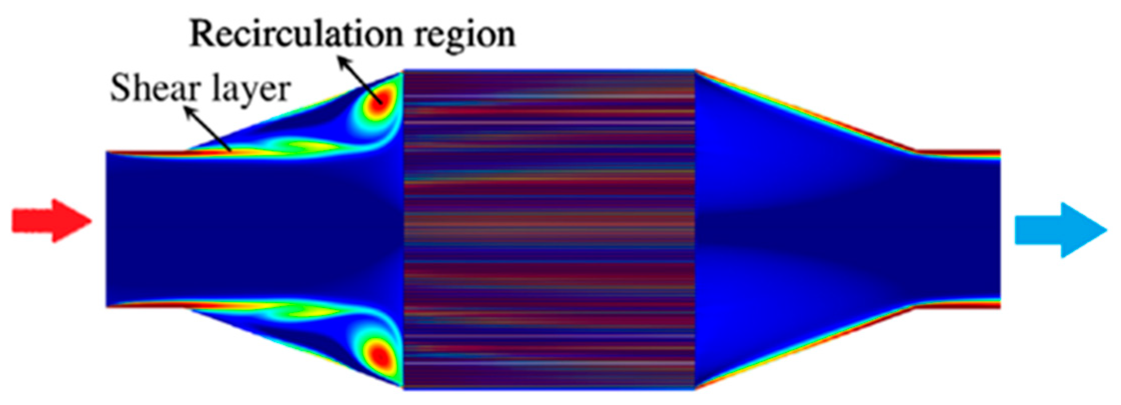
A linear cone is the simplest way to connect the inlet and outlet pipes to the monolith. However, if the expansion angle of the linear cone is large, the flow will separate, creating a recirculation zone between the inlet and monolith that deteriorates the uniformity of the flow. Figure 2 depicts a classic example of the flow features inside an automotive catalytic converter. In the inlet cone, the flow expands and forms a recirculation zone [12,13,14]. At the expansion inlet, a turbulence-free shear layer develops. The main flow jet region appears close to the axis of symmetry, whereas a recirculation flow region appears immediately after the main flow jet passes the inlet of the expansion; this intense recirculation induces high energy dissipation rates within the region of separated flow [15]. In contrast, the flow within the monolith channel is significantly simpler than the flow outside the channel. The channel flow becomes laminar as a result of viscous forces inside the narrow channels, and the characteristic Reynolds number in the channel typically does not exceed 500 [16], causing a significant pressure drop across the channel that can reach 66% of the overall pressure drop [7], whereas the pressure drop caused by the inlet cone is only approximately 13% [10]. Then, at the outlet cone, the cross section contracts, and the flow enters the outlet pipe.
In terms of the flow uniformity, Ma et al. [18] found that the exhaust flow in a conventional DPF tends to concentrate in the center, that is, more than 88% of the flow passes through less than 53% of the filter cross-sectional area. Accordingly, they proposed a streamlined cone with a reduced installation space using a unipolar sigmoid function; their cone permits a streamlined flow that avoids the need for a recirculation zone, increases the uniformity of the velocity by approximately 30%, and reduces the pressure drop by approximately 10% [18]. The flow uniformity inside the catalytic convertor has also been widely studied. The flow distribution worsens with an increase in both the inlet flow rate and the angle of divergence of the inlet cone [16,19]. Conklin et al. further showed that flow non-uniformity caused by the generation of recirculation zones affects the overall monolith performance, especially during cold-start transient operations [20].
Howitt and Sekella [21] showed that the placement of different flow-tailoring devices upstream of the monolith could ensure a uniform flow distribution. However, flow-tailoring devices increase the pressure drop and thermal mass of the system, where the latter delays the catalyst light-off. Bella et al. introduced similar flow constraints into the diverging section of the inlet to improve the flow distribution across the monolith channels relative to the free-flow conditions (i.e., without flow constraints) [22].
Wendland and Matthes conducted a visualization study of a dual-bed catalyst on a fully transparent, steady-state test bench and designed an enhanced and diagonal (EDH) cone tube [23]. The experimental results showed that implementing an EDH cone can significantly reduce the pressure drop and enable the catalyst structure to become more compact compared with a conventional cone. Kulkarni et al. studied the cone flow resistance in a TWC and found that an EDH cone can reduce the cone pressure drop by up to 62% in simulations [24]. Stratakis and Stamatelos demonstrated that the flow maldistribution is significantly influenced by the presence of a diffuser and a catalytic converter upstream of the filter and found that a diagonal cone can improve the air flow distribution and reduce the overall pressure drop [25], although the cone requires a sufficient amount of installation space.
Reducing the expansion angle of the inlet cone represents another method for reducing the flow maldistribution [26]. However, as with a diagonal cone, this approach requires a long diffuser and thus will be limited by space and design constraints in a typical automotive exhaust architecture. This issue becomes even more significant if the catalytic convertors are mounted close to the engine (i.e., to minimize cold-start emissions). In these compact packaged convertors, the monolith close to the engine due to the installation limit can lead to widely non-uniform flow behaviour [27,28], as shown in Figure 1, the compact design will potentially affect the performance due to this non-uniformity.
The cone affects not only the flow uniformity and pressure drop but also the regeneration temperature. Jiaqiang et al. [29] contrasted the distributions of the radial and axial temperatures with three different cones on the same DPF and showed that a cone with a better flow distribution has a lower temperature gradient and thus a longer service life.
Although the pressure drop directly caused by a cone contributes only slightly to the overall pressure drop [10], optimizing the cone structure will have a significant impact on the distribution of flow into the monolith, thereby improving the performance. With regard to cone optimization, a comprehensive view must be adopted given that the transport and deposition of particles, the thermal management, the pressure drop, and even the catalyst effectiveness are all related to the flow uniformity.
Non-uniform rational B-splines (NURBS) cones, which actively reduce the flow resistance, are currently being used in the simulation meshing and manufacturing of complex surfaces, such as ship design (i.e., the bulbous bow) and impeller blades [30,31,32]. The NURBS cone is a new cone design structure that requires less space than a sigmoid cone and achieves a higher flow uniformity based on simulation results; moreover, it is capable of reducing the overall pressure drop by up to 18% [33].
This work aims to validate the influence of the NURBS cone using a test bench by comparing the NURBS cone with the conventional cone via simulation and determining how the NURBS cone changes the flow before it passes through the monolith.
2. Experiment Procedure
2.1. Experimental Equipment
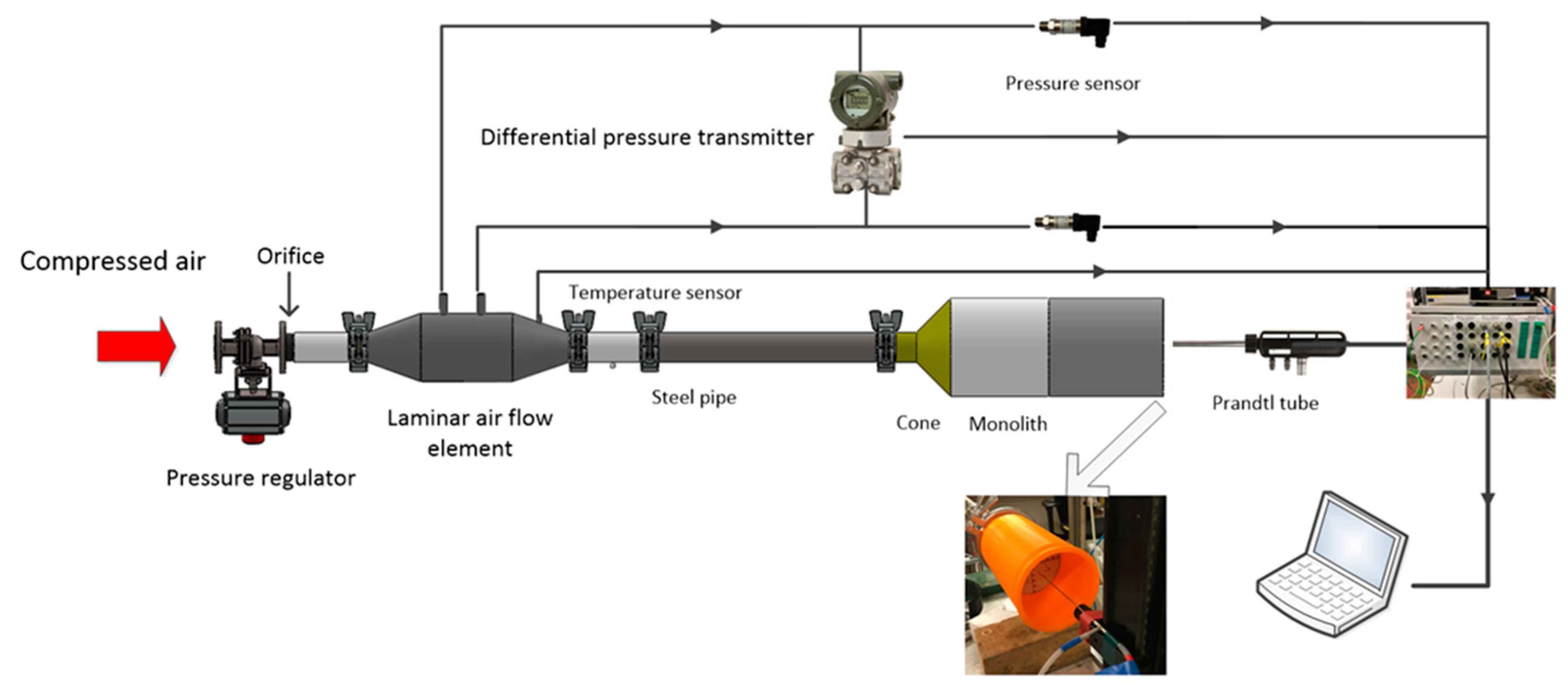
The experimental setup is shown in Figure 3.
In the laboratory, compressed and dried air was controlled and led through a flow restrictor and a laminar air flow element (Tsukasa Sokken, LFE-50B), which was connected to a differential pressure transmitter (Yokogawa, EJA110E) and two pressure sensors (VEGA, VEGABAR 14). After passing through a 1-meter-long steel pipe, the gas will reach the cone and then the monolith, after which it will travel through a straight pipe with a length of 15 cm before being emitted into the ambient atmosphere. At the outlet of the monolith, a Prandtl tube was used to measure the velocity on the outlet surface by connecting it to a micro-manometer (Furness Controls, FC014). To avoid disturbances from the channels on the sampling, the distance between the outlet surface and the position at which data were collected was 40 mm. All the data were acquired and recorded using LabView from National Instruments.
Two different monoliths were used in this study: one open substrate with a diameter of 90 mm, a length of 95 mm, and a density of 400 cells per square inch (CPSI) and one wall-flow filter, namely, a gasoline particulate filter (GPF), with a diameter of 104 mm, a length of 140 mm, and a density of 300 CPSI. Both substrates were made of cordierite and acquired from Corning. Two different steel pipes with inner diameters of 21 mm and 27.3 mm were used.
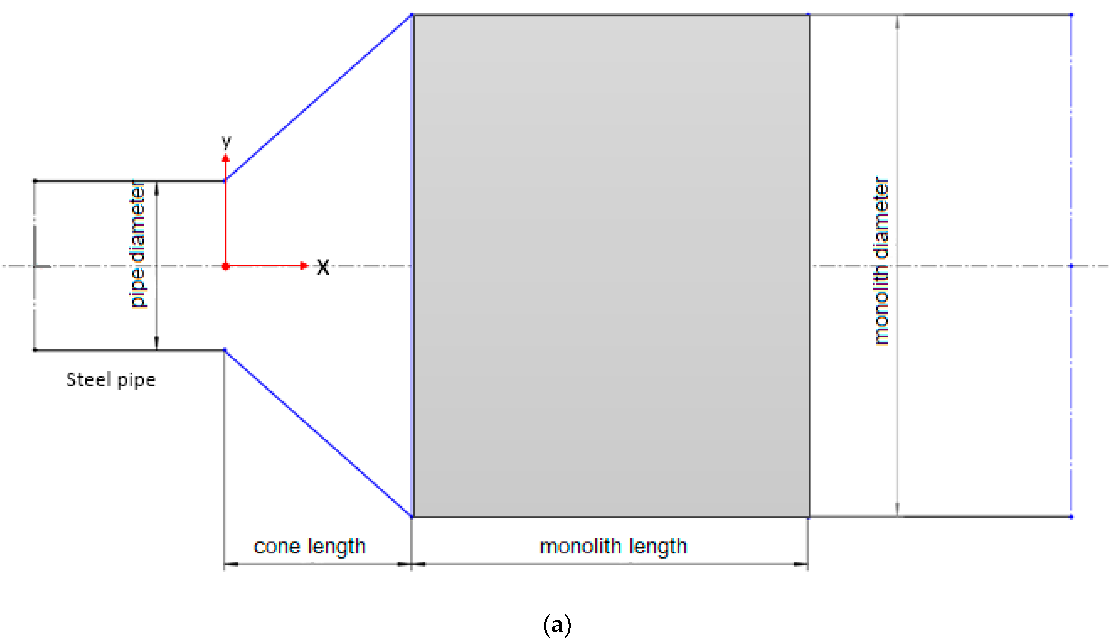
Two different expansion angles were used for the cones. The expansion angle α was 45° for Cones 3–6, whereas it was approximately 47° for Cones 1 and 2. To fit the steel pipe and monolith, 6 cones were manufactured via 3D printing, as shown in Table 1. The cone shape and the printed cones can be seen in Figure 4 and Figure 5.
Two different cone shapes, namely, conventional and NURBS, were employed. The conventional cone is a straight cone, whereas the NURBS cone is a type of streamlined cone drawn in 2D drawing and meshing software (Gambit 2.4.6) by choosing points along the flow lines according to the simulation results of the conventional cones. The simulation process was repeated several times to find the fittest NURBS curve to avoid the recirculation zone Because different velocities will generate different flow profiles, one representative velocity (average velocity of 16.5 m/s in the inlet pipe) was used for the NURBS design, 16.5 m/s corresponded to a single cylinder diesel engine, Changchai L12 with displacement 0.604 L, its speed at max. torque is 1920 r/min, and the diameter of exhaust pipe is 27.3 mm. To evaluate the effects of different flows, three different velocities were studied, and a total of 18 experiments were performed. The flows were generated by controlling the inlet pressure to the system (left side of Figure 3); because the different cones and substrates exhibit different pressure drops, the flow will change accordingly. However, by installing an orifice (which provides the major pressure drop), the changes in velocities due to different cones and substrates will be minor.
2.2. Velocity Measurements
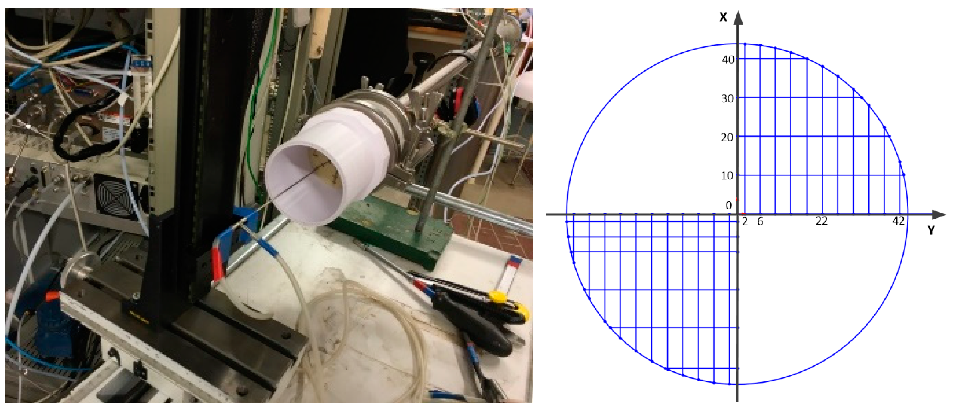
A Prandtl tube was used to acquire velocity measurements at different positions. The centre was chosen as the origin of the coordinate system. Taking Cone 3 as an example, the sampling positions in the first quadrant are shown in Figure 6. The points were set at intervals of 10 mm in the vertical direction and either 2 or 4 mm in the horizontal direction. The radius encompassing all the sampling positions was calculated and used for the analysis. To ensure that the flow was symmetrical and that the data were reliable, some measurement points in the third quadrant were repeated. During the measurement process, some disturbances (observed as variations and noise) were observed close to the outlet, and those disturbances were noted as being significantly reduced when sampling 40 mm after the monolith. Therefore, the sampling position was set at 40 mm away from the monolith outlet.
During the acquisition of measurements, the volumetric flow was set via the pressure regulator; the resulting volumetric flows are shown in Table 2. Due to previous contamination, the laminar flow element could not be used; hence, the volumetric flow was obtained by integrating the measured velocity data along the cross section. Case 7 is illustrated in Figure 7 as an example. In this case, when the distance to the center is 33 mm, the circular area occupies 54% of the cross-sectional area of the monolith, but more than 75% of the flow passes through it. This value is somewhat smaller than that obtained by Ma et al. [18], but it is still an obvious problem when considering flow uniformity. As can be seen in Figure 7, the velocity increases close to the border. This phenomenon has been observed many times in the literature and will be discussed in detail in Section 4.2 and Section 4.4.
From the scatter of the velocities and an analysis of the measurements acquired from different quadrants, the flow was confirmed to be symmetrical.
3. Model Formulation
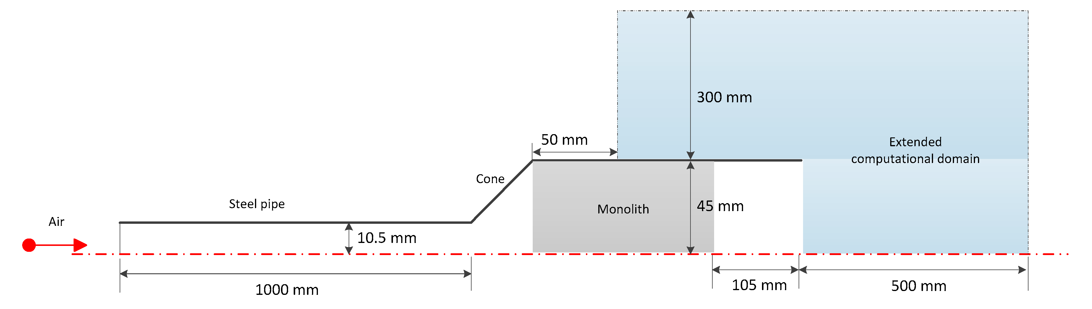
Figure 8 shows an axisymmetric version of the domain used in the 2D simulation of Cone 1. The computational domain was intentionally extended to ensure fully developed flow. The monolith, which is an un-washed and coated model, has square cross section channels with side lengths of 1.1 mm and a wall thickness between the channels of 0.1 mm, corresponding to a monolith with a density of 400 CPSI.
This work focuses on the fluid dynamics and turbulence inside the monolith for cold flow, i.e., without chemical reactions or thermal effects. Hence, the mass and momentum conservation equations are sufficient to describe the problem [34]. The modelling can be separated into two parts: the open sections and the monolith.
3.1. Modeling of the Open Section
In all cases, the flow was assumed to be incompressible and statistically stationary; hence, the steady-state Reynolds-averaged Navier–Stokes (RANS) equations were used to describe the turbulence. The open sections consist of the domains both before and after the monolith.
The RANS mass conservation equation is [35]:
The momentum conservation equation, where the closure is provided through a turbulence viscosity model, is:
where:
The Menter shear stress transport (SST) model is applied for the turbulence. The turbulence model is combined with the turbulence model insofar that the model is used in the inner region of the boundary layer, whereas the model is used for free shear flow [36,37,38].
The turbulence viscosity is described by Equation (4), and transport equations are taken from the Wilcox model [39,40], in Equations (5) and (6), respectively.
Far from the wall, the transport equation is obtained by substituting into the transport equation, leading to a modified transport equation with the addition of a cross-diffusion term [40].
3.2. Modeling of the Monolith
A DOC monolith is composed of approximately 5257 small channels, whereas a GPF monolith has more than 7020 channels. Because these channels have the same geometry and the channel diameter is considerably smaller than the filter diameter D, which satisfies the criteria for a porous medium without considering flow in channels, the monolith can be regarded as a homogeneous porous medium.
The mass conservation equation in Equation (1) is also valid for this section of the domain. Meanwhile, the momentum conservation equations, namely, the volume-averaged Navier–Stokes (VANS) equations, a source term is added to the right-hand side of Equation (2), resulting in Equation (7) [41]:
The source term contains viscous resistance (Darcy term) and inertial resistance (Forchheimer term). The inertial resistance has an obvious influence only when the percolation velocity of the filter wall is high [42]. In the diesel exhaust range, the percolation velocity generally does not exceed 0.2 m/s; in this paper, the percolation velocity is less than 0.01 m/s and, thus, the influence of the Forchheimer term can be ignored. Furthermore, can be set to 0 when considering only viscous resistance. In the calculations, porous media have no effect on generation and the dissipation of turbulence.
The main parameters of the porous media are the axial and radial permeabilities. Hayes et al. found that by setting the radial permeability at least 100 times higher than the axial permeability, the radial velocity is negligible, as in a real monolith [43]. The radial permeability is related to the size of the channels according to Equation (9) if Poiseuille flow is assumed [44]:
3.3. Grid Refinement and Validation
The structural parameters of the cone depend on the experimental parameters. The domain was meshed by block-structured meshes that were refined close to the wall in Gambit. The grid independence was tested based on the velocity magnitude after the monolith. The grids differed slightly among the different cases. Taking Case 7 as an example, grids with 277,500, 309,725, and 314,600 control volumes were used. After the grid test, the peak velocity after the monolith changed by less than 1% between the final two grids; thus, the grid with 309,725 control volumes, including 70,215 control volumes in the extended computational domain, was chosen with a 0.2 mm grid spacing near the monolith border.
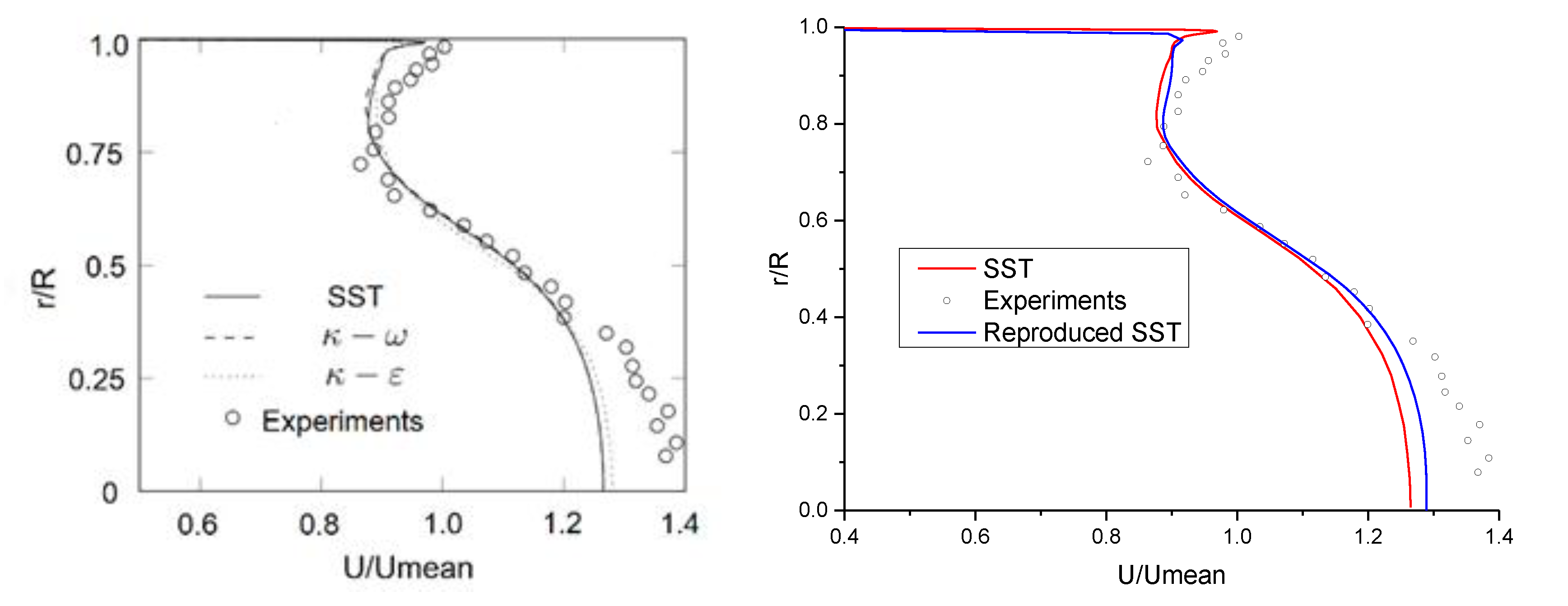
Hayes et al. and Cornejo et al. studied various turbulence models and performed comparisons with experimental data [43,45,46]. Their findings were quite similar to the experimental results shown in Figure 9, and they attributed the observed errors to the limitations of the RANS models. They chose the SST model because it exhibits better agreement with the experimental data for a finer mesh. The model in this study was verified according to the same procedure used in the aforementioned report by Hayes et al. [43]. Differences near the border and central parts were ignored because the measurement errors that occur during the experiment, especially in the flow near the border, could be influenced easily by the Prandtl tube.
The reproduced model was validated by comparison with the experimental data from Case 7. The settings and boundary conditions used in the simulations are summarized in Table 3. The calculation was performed using Fluent 18.0.
4. Results and Discussion
4.1. Pressure Drop
As shown in Table 2, the volumetric flows of a conventional cone and a NURBS cone of the same size are slightly different. To eliminate errors caused by the structural differences between a GPF and a DOC, the ratio of the pressure drop per volumetric flow is used in Table 4, where the pressure drop is the absolute pressure from the back-pressure sensor, and the space velocity is the volumetric flow divided by the monolith volume.
Table 4 shows that the pressure drops per volumetric flow of the NURBS cones are lower than those of the conventional cones to different extents, with the largest reduction being 12%. This result is obtained because the NURBS cone efficiently reduces the generation of recirculation zones within the cone and makes the flow into the monolith more uniform. The reduction ratio is the pressure drop per volumetric flow of the NURBS cone divided by the corresponding value of the conventional cone. The reduction ratio changes irregularly at different velocities. One reason for this result is that the NURBS curve is drawn under the simulation of a constant inlet velocity of 16.5 m/s. The maximum reduction case has similar initial conditions, which also represents the flow complexity. It can also be noted that the reduction ratio of the GPF is smaller than the DOC. This is due to the cone volume and the monolith volume of GPF all being bigger than the DOC, which provides enough space to develop the flow and make the flow more uniform and undermine the difference caused by NURBS cone.
4.2. Velocity Profile
Figure 6 shows the experimental velocities collected at intervals along the radial position on the outlet surface for the cones under different inlet velocities. The velocities were collected from the first quadrant of the monolith’s outlet surface.
Figure 10, Figure 11 and Figure 12 show comparisons between the conventional cones and NURBS cones. In the central part of the outlet, the maximum velocities from the NURBS cones are all smaller than those from the conventional cones, and a stark contrast is observed near the border. These experimental differences demonstrate that the NURBS cone can result in a more uniform flow and can reduce the amount of flow passing through the central part.
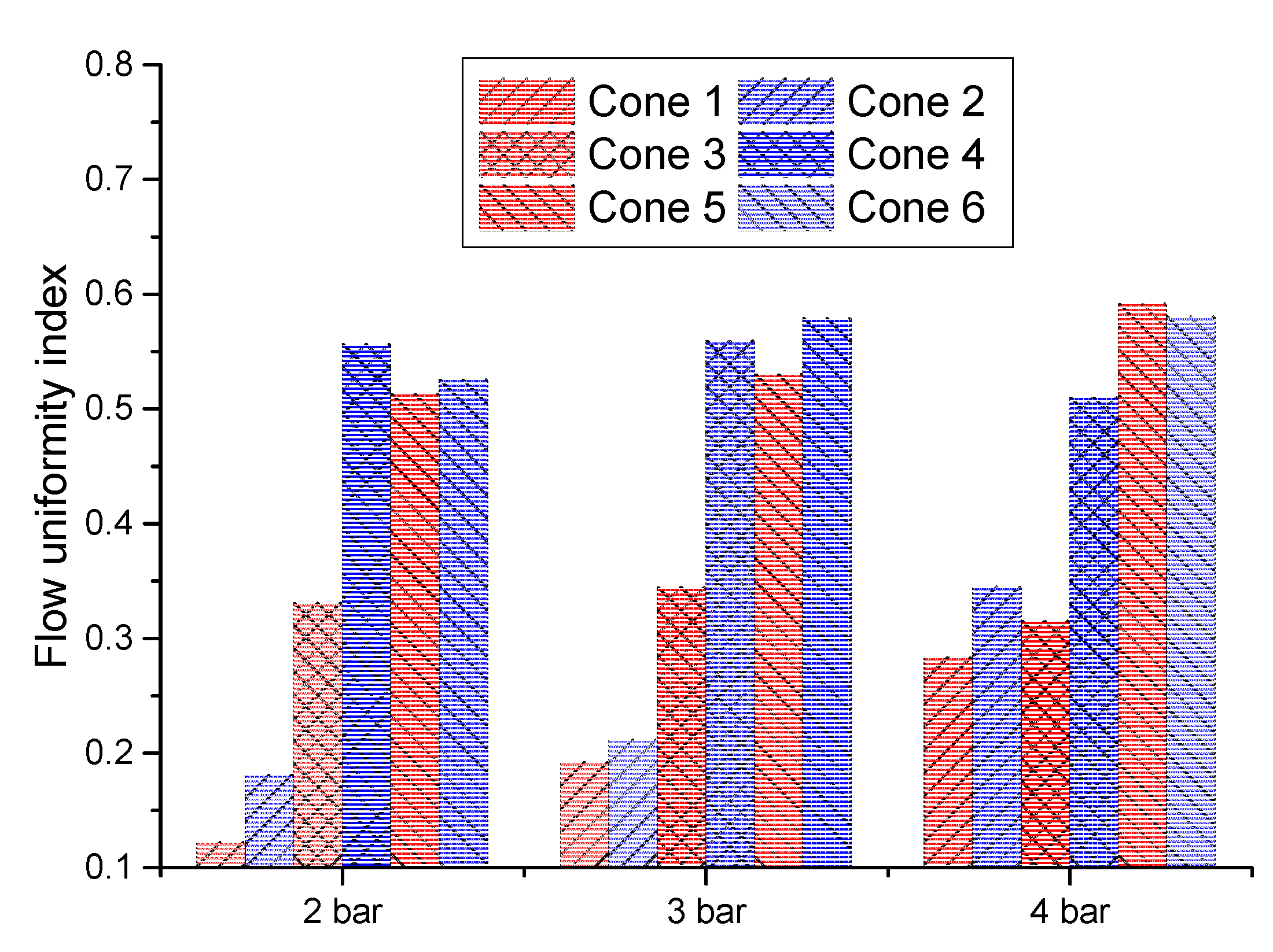
4.3. Flow Uniformity
When modelling catalytic converters, it is common practice to use a single-channel approach, which assumes the same temperature and residence times among all the channels. The flow uniformity index can be used to assess this assumption. The NURBS cone can improve the flow uniformity, which is also important for the deposition of PM. The flow uniformity index is used to reveal the difference in the flow distribution [26].
where is the flow uniformity index with values between 0 and 1 (1 being the best), n is the total number of measurement points, and is the mean velocity in the cross section, which can be obtained from the volume divided by the area.
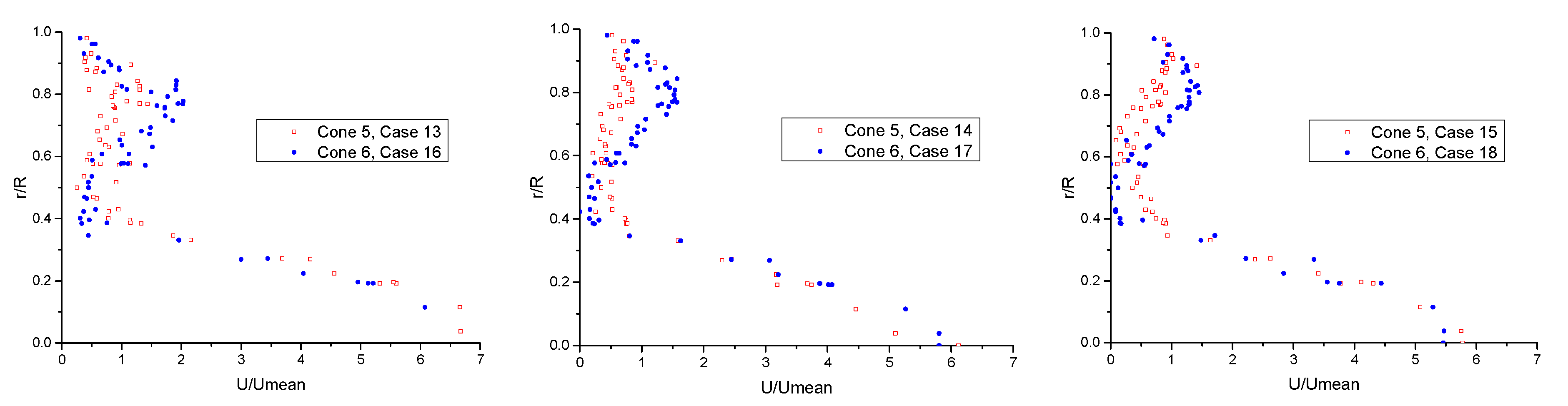
The results in Figure 13 show that in most cases, the NURBS cone has a positive influence on the flow uniformity. However, in a comparison between Case 15 and Case 18 (4 bar, GPF substrate), the NURBS cone did not show better results. One reason could be that the NURBS curve is designed for a specific and constant inlet velocity; therefore, the streamlined NURBS cone designed for lower velocities would not always exhibit a better performance when switching to higher velocities.
4.4. CFD Velocity Profiles
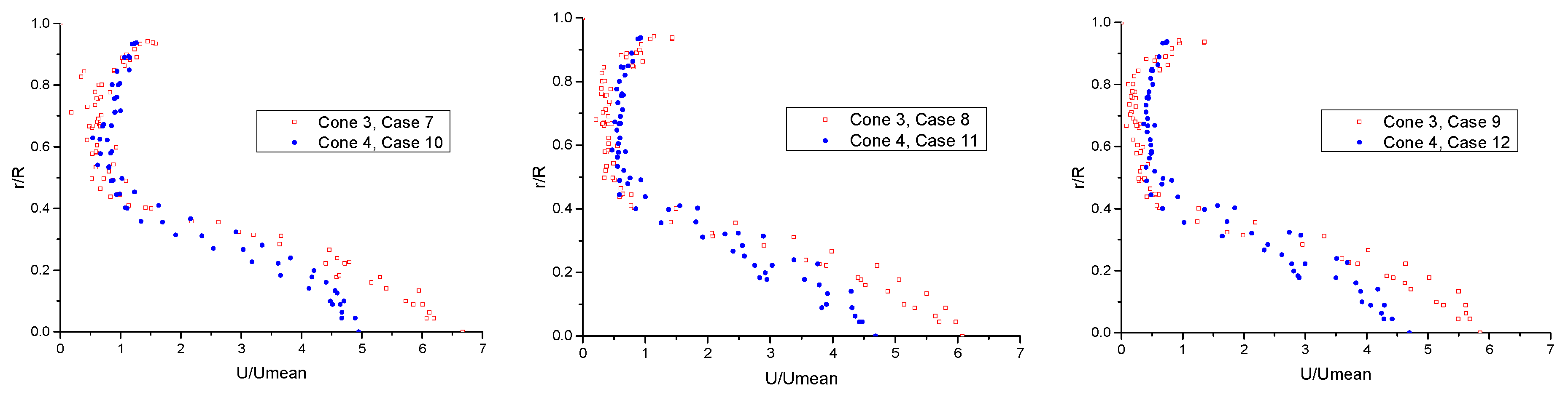
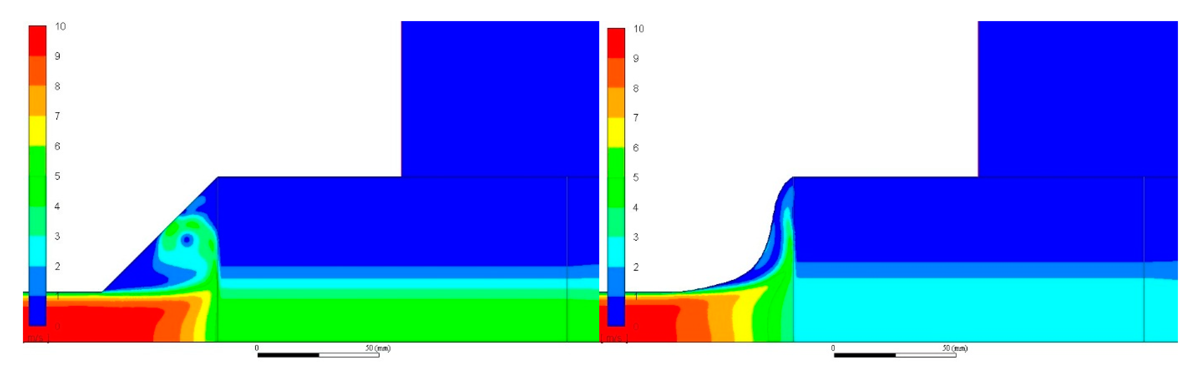
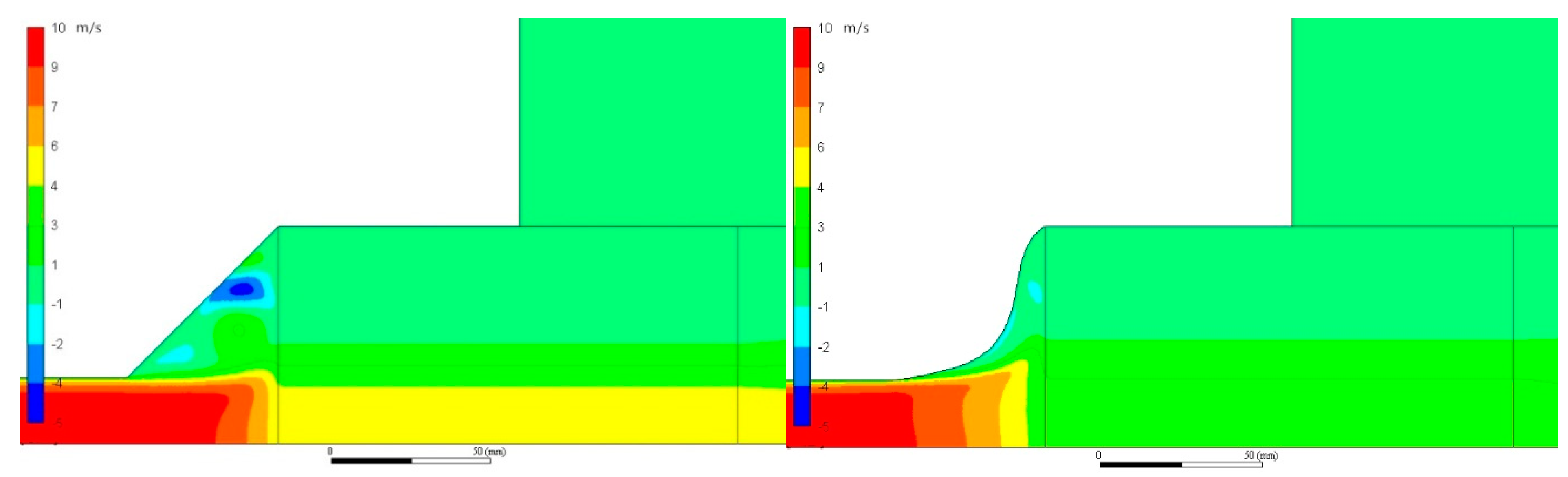
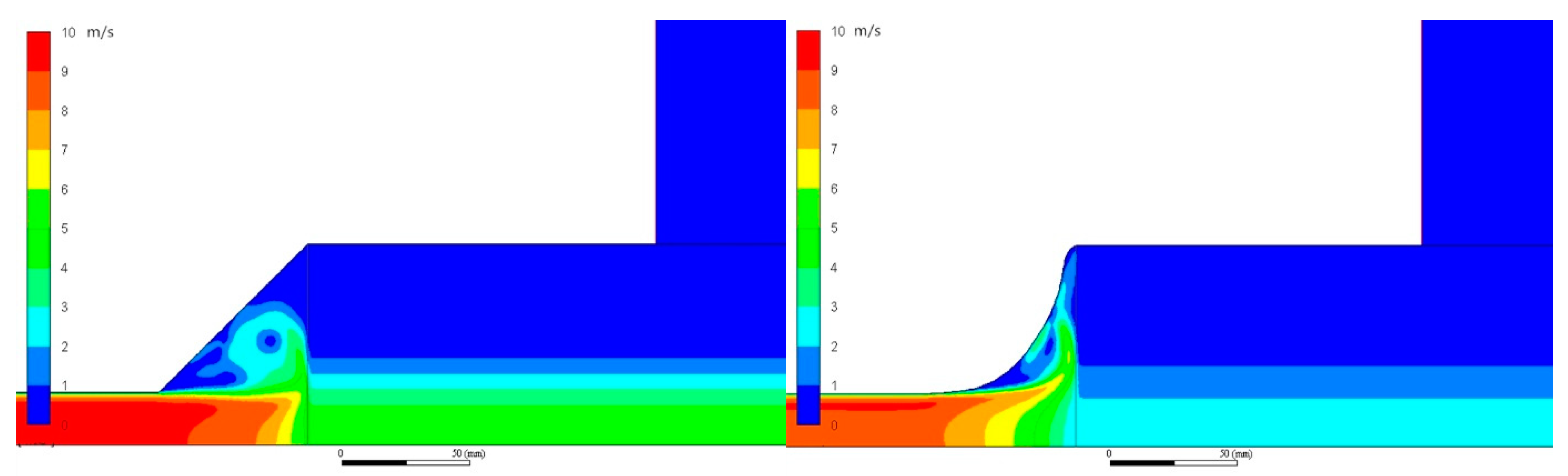
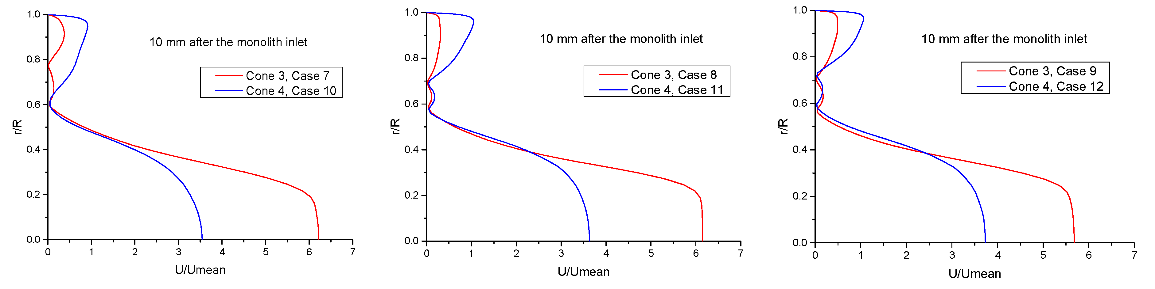
To more accurately quantify the flow uniformity and obtain further insight into the influence of the cone on the flow, a simulation is required in combination with the experimental results to determine how the flow changes before it enters the monolith. Accordingly, the cause of the large difference between Cones 3 and 4 can be determined. Figure 14 and Figure 15 show comparisons of the velocity magnitudes and axial velocities between Case 7 and Case 10 from the simulation results, and Figure 16 shows a comparison of the velocity magnitudes between Case 13 and Case 16.
Figure 17 shows the velocity profiles (containing both the axial velocity and the radial velocity) at 10 mm after the monolith inlet from the simulation results.
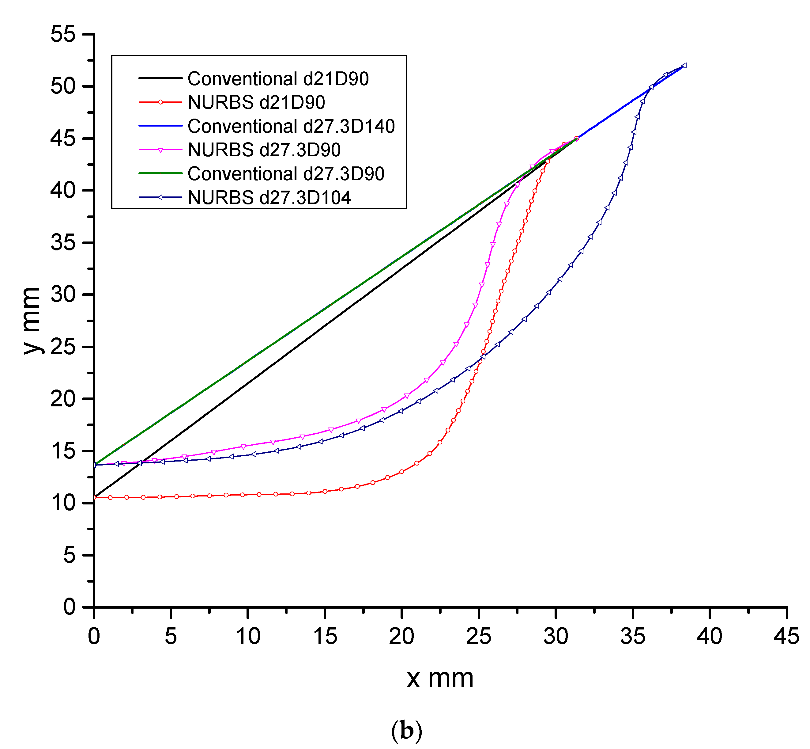
As shown in Figure 17, the maximum velocity of the NURBS cone (Cone 4) and the values near the centre are smaller than those of the conventional cone (Cone 3), and the value near the border is higher, which allows the NURBS cone to achieve better flow uniformity.
Along the radial position, the velocity in the conventional cone (Cone 3) changes abruptly at approximately r/R = 0.2 in all three cases, whereas that in the NURBS cone does not. This difference occurs because the NURBS cone expands gradually and does not exhibit a large recirculation zone, while the conventional cone does. Furthermore, the wall exerts a viscous drag force on the flow as it expands, which yields a better flow distribution.
In addition, velocity variations occur between r/R = 0.6 and 0.8, particularly for Cone 3, as shown in Figure 17. These variations were caused by the recirculation zone in the cone, which can be seen in Figure 14 and Figure 15. However, at the lowest velocity, which occurs in Case 10, the velocity exhibits a different pattern, which means that the initial velocity can also influence the formation of recirculation zones.
The NURBS cone provides a smooth connection between the exhaust pipe and the monolith and reduces the recirculation zone, thereby allowing additional flow to pass through the border position; as a result, the NURBS cone exhibits a higher velocity than the conventional cone.
Figure 18 depicts the changes in the simulated velocity magnitude from the monolith inlet to 40 mm after the monolith, where the velocity magnitude contains both the axial velocity and the radial velocity.
The large difference in the velocities between the monolith inlet and the measurement position 10 mm after the monolith inlet shows how the flow changes within the inlet cone. On the inlet surface, there is substantial radial flow from r/R = 0.3 to 0.7, as the blocking effect of the monolith and the expansion of the cone result in the generation of a recirculation zone.
The profiles for the position 10 mm after the monolith inlet and the monolith outlet are quite similar, which means that the flow inside the monolith is stable. Moreover, compared with the conventional cone (Cone 3), the NURBS cone (Cone 4) does not exhibit a clear recirculation zone, as the recirculation zone caused variation in the region of r/R = 0.6 to 0.8 for Cone 3.
The velocity near the border exhibits a peak 40 mm after the monolith outlet. However, the profile at this position is still not identical to the experimental profile. This discrepancy may have been caused by the Prandtl tube, as the diameter of the Prandtl tube is approximately 1.3 mm, while the channel diameter is 1.1 mm. Consequently, the flow will be disturbed by the Prandtl tube and by the holder when moving the Prandtl tube to the border position.
4.5. Future Work
All experiments and simulations in this paper were performed at room temperature. The reason for this is that the cones were printed in plastic, and also for this paper the main target is to assess the cone’s influence on flow field. If considering high temperatures, like 600 °C, under the same flow conditions, the flow viscosity will decrease, the velocity would increase, and the effect of the NURBS cone will need to be confirmed with more simulations in future.
An important aspect that needs to be studied in the future is the influence of the NURBS cone on heat dissipation during gasoline particulate filter regeneration or catalytic reactions. The next step will be to study the thermal effects and pressure drop due to the flow maldistribution. A detailed understanding of the flow field during particle capture is of utmost important to assure high performance of future powertrains.
5. Conclusions
In this paper, the influence of a cone on the flow distribution was studied via both experiments and simulations. A non-uniform rational B-splines (NURBS) cone was proposed for use in the design of the cone.
Several cones were fabricated and tested comparatively. A NURBS cone can improve the flow uniformity in the monolith with a pressure drop reduction reaching 12% under certain conditions. However, the reduced pressure drops varied at different velocities and with different cones due to the changes in the flow within the cone when the initial conditions changed. However, the NURBS cone was designed in reference to a constant velocity and configuration. A specific design is thus required for each specific case to achieve the best results.
Moreover, the flow conditions before the monolith were analyzed via simulations. The NURBS cone enables a streamlined flow by avoiding the separation zone, creates less recirculation, and has a positive influence on the pressure drop.
In summary, the NURBS cone is a suitable choice for cone design applications. NURBS cones can reduce the required installation space, and they have potential for future applications in other after-treatment systems.
Author Contributions
Conceptualization, M.M. and X.L.; methodology, M.M. and J.S.; software, M.M. and H.S.; validation, M.M. and J.S.; formal analysis, M.M.; investigation, M.M. and X.L.; resources, J.S.; data curation, M.M. and J.S.; writing—original draft preparation, M.M.; writing—review and editing, J.S. and. H.S.; supervision, J.S.; project administration, J.S.; funding acquisition, J.S.
Funding
This research was funded by Chalmers University of technology, 2018. This work is supported in part by a scholarship from the China Scholarship Council (CSC) under Grant File No. 201706020106.
Acknowledgments
All technical staff at the division of Combustion and Propulsion Systems are deeply acknowledged, including Patrik Wåhlin for printing the cones and Timothy Benham, Anders Mattsson, Robert Buadu and Dr. Alf-Hugo Magnusson for building the test bench.
Conflicts of Interest
The authors declare no conflict of interest.
Nomenclature
| Reynolds-averaged velocity (m/s) | |
| Time (s) | |
| Pressure (Pa) | |
| Strain tensor (1/s) | |
| Inertial resistance factor | |
| Identity matrix | |
| Channel hydraulic diameter (m) | |
| Permeability (m2) | |
| Wilcox —ω model parameter | |
| Wilcox —ω model parameter | |
| Wilcox —ω model parameter | |
| Rate of viscous dissipation (m2/s2) | |
| Turbulence kinetic energy (m2/s2) | |
| Viscosity (Pa) | |
| Turbulence viscosity (Pa·s) | |
| Density (kg/m3) | |
| Turbulence Prandtl number for ω | |
| Turbulence Prandtl number for | |
| Monolith porosity | |
| Specific dissipation ratio |
Abbreviations
| EATS | Exhaust after-treatment system |
| DOC | Diesel oxidation catalyst |
| DPF | Diesel particulate filter |
| GPF | Gasoline particulate filter |
| SCR | Selective catalytic reduction |
| LNT | Lean NOx trap |
| PM | Particulate matter |
| RANS | Reynolds-averaged Navier–Stokes equations |
| VANS | Volume-averaged Navier–Stokes equations |
References
- Meloni, R.; Naso, V. An insight into the effect of advanced injection strategies on pollutant emissions of a heavy-duty diesel engine. Energies 2013, 6, 4331–4351. [Google Scholar] [CrossRef]
- Raza, M.; Chen, L.F.; Leach, F.; Ding, S.T. A review of Particulate Number (PN) emissions from Gasoline Direct Injection (GDI) engines and their control techniques. Energies 2018, 11, 1417. [Google Scholar] [CrossRef]
- Okubo, M.; Kuroki, T.; Kawasaki, S.; Yoshida, K.; Yamamoto, T. Continuous regeneration of ceramic particulate filter in stationary diesel engine by Nonthermal-Plasma-Induced ozone injection. IEEE Trans. Ind. Appl. 2009, 45, 1568–1574. [Google Scholar] [CrossRef]
- Wang, D.; Liu, Z.C.; Tian, J.; Liu, J.W.; Zhang, J.R. Investigation of particle emission characteristics from a diesel engine with a diesel particulate filter for alternative fuels. Int. J. Automot. Technol. 2012, 13, 1023–1032. [Google Scholar] [CrossRef]
- Zhang, B.E.J.; Gong, J.; Yuan, W.; Zhao, X.; Hu, W. Influence of structural and operating factors on performance degradation of the diesel particulate filter based on composite regeneration. Appl. Therm. Eng. 2017, 121, 838–852. [Google Scholar] [CrossRef]
- Laurell, M.; Sjörs, J.; Ovesson, S.; Lundgren, M. The innovative exhaust gas aftertreatment system for the new Volvo 4 Cylinder Engines; a unit catalyst system for gasoline and diesel cars. In Proceedings of the 22nd Aachen Colloquium Automobile and Engine Technology, Aachen, Germany, 2–3 July 2015. [Google Scholar]
- Konstandopoulos, A.G.; Skaperdas, E.; Masoudi, M. Inertial contributions to the pressure drop of diesel particulate filters. SAE Tech. Pap. 2001. [Google Scholar] [CrossRef]
- Haralampous, O.A.; Kandylas, I.P.; Koltsakis, G.C.; Samaras, Z.C.; Haralampous, O.A. Diesel particulate filter pressure drop Part 1: Modelling and experimental validation. Int. J. Engine Res. 2004, 5, 149–162. [Google Scholar] [CrossRef]
- Masoudi, M. Pressure drop of segmented diesel particulate filters. SAE Tech. Pap. 2005. [Google Scholar] [CrossRef]
- Torregrosa, A.J.; Serrano, J.R.; Arnau, F.J.; Piqueras, P. A fluid dynamic model for unsteady compressible flow in wall-flow diesel particulate filters. Energy 2011, 36, 671–684. [Google Scholar] [CrossRef] [Green Version]
- Myung, C.L.; Kim, J.; Jang, W.; Jin, D.; Park, S.; Lee, J. Nanoparticle filtration characteristics of advanced metal foam media for a spark ignition direct injection engine in steady engine operating conditions and vehicle test modes. Energies 2015, 8, 1865–1881. [Google Scholar] [CrossRef]
- Shuja, S.Z.; Habib, M.A. Fluid flow and heat transfer characteristics in axisymmetric annular diffusers. Comput. Fluids 1996, 25, 133–150. [Google Scholar] [CrossRef]
- Ubertini, S.; Desideri, U. Experimental performance analysis of an annular diffuser with and without struts. Exp. Therm. Fluid Sci. 2000, 22, 183–195. [Google Scholar] [CrossRef]
- Neve, R.S. Computational fluid dynamics analysis of diffuser performance in gas-powered jet pumps. Int. J. Heat Fluid Flow 1993, 14, 401–407. [Google Scholar] [CrossRef]
- Forrester, S.E.; Evans, G.M. Computational modelling study of the hydrodynamics in a sudden—Tapered contraction reactor geometry. Chem. Eng. Sci. 1997, 52, 3773–3785. [Google Scholar] [CrossRef]
- Karvounis, E.; Assanis, D.N. The effect of inlet flow distribution on catalytic conversion efficiency. Int. J. Heat Mass Transf. 1993, 36, 1495–1504. [Google Scholar] [CrossRef]
- Ozhan, C.; Fuster, D.; Da Costa, P. Multi-scale flow simulation of automotive catalytic converters. Chem. Eng. Sci. 2014, 116, 161–171. [Google Scholar] [CrossRef]
- Ma, L.; Paraschivoiu, M.; Yao, J.; Blackman, L. Improving flow uniformity in a diesel particulate filter system. SAE Tech. Pap. 2001. [Google Scholar] [CrossRef]
- Lai, M.C.; Kim, J.Y.; Cheng, C.Y.; Li, P.; Chui, G.; Pakko, J.D. Three-dimensional simulations of automotive catalytic converter internal flow. SAE Trans. 1991, 100, 241–250. [Google Scholar]
- Chakravarthy, V.K.; Conklin, J.C.; Daw, C.S.; D’Azevedo, E.F. Multi-dimensional simulations of cold-start transients in a catalytic converter under steady inflow conditions. Appl. Catal. A-Gen. 2003, 241, 289–306. [Google Scholar] [CrossRef]
- Howitt, J.S.; Sekella, T.C. Flow effects in monolithic honeycomb automotive catalytic converters. SAE. Tech. Pap. 1974. [Google Scholar] [CrossRef]
- Bella, G.; Rocco, V.; Maggiore, M. A study of inlet flow distortion effects on automotive catalytic converters. J. Eng. Gas Turbines Power 1991, 113, 419. [Google Scholar] [CrossRef]
- Wendland, D.W.; Matthes, W.R. Visualization of automotive catalytic converter internal flows. SAE. Tech. Pap. 1986. [Google Scholar] [CrossRef]
- Kulkarni, G.S.; Singh, S.N.; Seshadri, V.; Mohan, R. Optimum diffuser geometry for the automotive catalytic converter. Indian J. Eng. Mater. Sci. 2003, 10, 5–13. [Google Scholar]
- Stratakis, G.A.; Stamatelos, A.M. Mow maldistribution measurements in wall-flow diesel filters. Proc. Inst. Mech. Eng. Part D-J. Automob. Eng. 2004, 218, 995–1009. [Google Scholar] [CrossRef]
- Weltens, H.; Bressler, H.; Terres, F.; Neumaier, H.; Rammoser, D. Optimisation of catalytic converter gas flow distribution by CFD prediction. SAE. Tech. Pap. 1993. [Google Scholar] [CrossRef]
- Badami, M.; Millo, F.; Zuarini, A.; Gambarotto, M. CFD analysis and experimental validation of the inlet flow distribution in close coupled catalytic converters. SAE Tech. Pap. 2003. [Google Scholar] [CrossRef]
- Salasc, S.; Barrieu, E.; Leroy, V. Impact of manifold design on flow distribution of a close-coupled catalytic converter. SAE Tech. Pap. 2005. [Google Scholar] [CrossRef]
- Jiaqiang, E.; Liu, M.; Deng, Y.; Zhu, H.; Gong, J. Influence analysis of monolith structure on regeneration temperature in the process of microwave regeneration in the diesel particulate filter. Can. J. Chem. Eng. 2016, 94, 168–174. [Google Scholar]
- Wang, X.R.; Wang, Z.Q.; Wang, Y.S.; Lin, T.S.; He, P. A bisection method for the milling of NURBS mapping projection curves by CNC machines. Int. J. Adv. Manuf. Technol. 2017, 91, 155–164. [Google Scholar] [CrossRef]
- Zhou, W.; Liu, B.; Wang, Q.; Cheng, Y.; Ma, G.; Chang, X.; Chen, X. NURBS-enhanced boundary element method based on independent geometry and field approximation for 2D potential problems. Eng. Anal. Bound. Elem. 2017, 83, 158–166. [Google Scholar] [CrossRef]
- Coelho, M.; Roehl, D.; Bletzinger, K.U. Material model based on NURBS response surfaces. Appl. Math. Model. 2017, 51, 574–586. [Google Scholar] [CrossRef]
- Mu, M.; Li, X.; Aslam, J.; Qiu, Y.; Yang, H.; Kou, G.; Wang, Y. A study of shape optimization method on connection cones for diesel particulate filter (DPF). In Proceedings of the ASME 2016 International Mechanical Engineering Congress and Exposition, Phoenix, AZ, USA, 11–17 November 2016; p. V012T16A001. [Google Scholar]
- Strom, H.; Sasic, S.; Andersson, B. Design of automotive flow-through catalysts with optimized soot trapping capability. Chem. Eng. J. 2010, 165, 934–945. [Google Scholar] [CrossRef]
- Versteeg, H.K.; Malalasekera, W. An Introduction to Computational Fluid Dynamics: The Finite Volume Method; Pearson Education Limited: Essex, UK, 2007. [Google Scholar]
- Menter, F.R. Two-equation eddy-viscosity turbulence models for engineering applications. Aiaa J. 1994, 32, 1598–1605. [Google Scholar] [CrossRef] [Green Version]
- Menter, F.R. Eddy viscosity transport equations and their relation to the k-ɛ model. J. Fluids Eng. 1997, 119, 876. [Google Scholar] [CrossRef]
- Ishak, M.H.H.; Ismail, F.; Che Mat, S.; Abdullah, M.Z.; Aziz, M.S.A.; Idroas, M.Y. Numerical analysis of nozzle flow and spray characteristics from different nozzles using diesel and biofuel blends. Energies 2019, 12, 281. [Google Scholar] [CrossRef]
- Wilcox, D.C. Reassessment of the scale-determining equation for advanced turbulence models. Aiaa J. 1988, 26, 1299–1310. [Google Scholar] [CrossRef]
- Wilcox, D.C. Turbulence Modeling for CFD; DCW Industries: Flintridge, CA, USA, 2006; pp. 363–367. [Google Scholar]
- Masoudi, M. Hydrodynamics of diesel particulate filters. SAE Tech. Pap. 2002. [Google Scholar] [CrossRef]
- Jiao, G.; Liu, H.; Yang, L.; Li, C. Simulation of catalytic combustion flows in honeycomb reactors. J. Beijing Univ. Chem. Technol. 2004, 2, 1–5. [Google Scholar]
- Hayes, R.E.; Fadic, A.; Mmbaga, J.; Najafi, A. CFD modelling of the automotive catalytic converter. Catal. Today 2012, 188, 94–105. [Google Scholar] [CrossRef]
- Ekström, F.; Andersson, B. Pressure drop of monolithic catalytic converters experiments and modeling. SAE Tech. Pap. 2003. [Google Scholar] [CrossRef]
- Cornejo, I.; Nikrityuk, P.A.; Hayes, R.E. Turbulence decay inside the channels of an automotive catalytic converter monolith. Emiss. Control Sci. Technol. 2017, 3, 302–309. [Google Scholar] [CrossRef]
- Cornejo, I.; Nikrityuk, P.A.; Hayes, R.E. Multiscale RANS-based modeling of the turbulence decay inside of an automotive catalytic converter. Chem. Eng. Sci. 2018, 175, 377–386. [Google Scholar] [CrossRef]
Figure 1.
Volvo diesel after-treatment system and an image highlighting its engine placement (right). Reproduced from [6], Aachen Colloquium Automobile and Engine Technology, 2015.
Figure 1.
Volvo diesel after-treatment system and an image highlighting its engine placement (right). Reproduced from [6], Aachen Colloquium Automobile and Engine Technology, 2015.

Figure 2.
Typical flow patterns inside a catalytic converter in the plane of symmetry. Reproduced from [17], Elsevier, 2014.
Figure 2.
Typical flow patterns inside a catalytic converter in the plane of symmetry. Reproduced from [17], Elsevier, 2014.

Figure 3.
Schematic of the experimental setup.

Figure 4.
The shapes of the cones.


Figure 5.
Printed cones. The yellow cones are Cones 1 and 2, the white cones are Cones 3 and 4, and the blue cones are Cones 5 and 6. The shape of the cones is depicted in Figure 4b.
Figure 5.
Printed cones. The yellow cones are Cones 1 and 2, the white cones are Cones 3 and 4, and the blue cones are Cones 5 and 6. The shape of the cones is depicted in Figure 4b.

Figure 6.
Prandtl sampling setup and sampling position schematic (right).

Figure 7.
Measured velocity on the outlet surface (Cone 3, Case 7).

Figure 8.
Schematic domain of the simulation.

Figure 9.
Simulated and experimental axial velocity profiles after the monolith was reproduced from [46], Elsevier, 2018 (left). The right figure shows a comparison between the simulations performed using the shear stress transport (SST) κ-ω model employed by Cornejo et al. and the authors’ reproduced SST κ-ω model.

Figure 10.
Comparison of DOC substrates using Cone 1 (conventional) and Cone 2 (NURBS) under different inlet velocities from the experimental results. The left figure shows the lowest velocities, while the right figure shows the highest velocities. The x-axis shows the normalized velocities in order to illustrate the flow uniformity. The actual velocities are given in Table 2.

Figure 11.
Comparison of DOC substrates using Cone 3 (conventional) and Cone 4 (NURBS) under different inlet velocities from the experimental results. The left figure shows the lowest velocities, while the right figure shows the highest velocities. The x-axis shows the normalized velocities in order to illustrate the flow uniformity. The actual velocities are given in Table 2.

Figure 12.
Comparison of GPF substrates using Cone 5 (conventional) and Cone 6 (NURBS) under different inlet velocities from the experimental results. The left figure shows the lowest velocities, while the right figure shows the highest velocities. The x-axis shows the normalized velocities in order to illustrate the flow uniformity. The actual velocities are given in Table 2.

Figure 13.
Comparison among the flow uniformity indexes from the experimental results. Red bars correspond to the conventional cones, and blue bars correspond to the NURBS cones.
Figure 13.
Comparison among the flow uniformity indexes from the experimental results. Red bars correspond to the conventional cones, and blue bars correspond to the NURBS cones.

Figure 14.
Contours of the velocity magnitude (Cases 7 and 10).

Figure 15.
Contours of the axial velocity (Cases 7 and 10).

Figure 16.
Contours of the velocity magnitude (Cases 13 and 16).

Figure 17.
Comparison of the velocities for Cones 3 and 4 at 10 mm after the monolith inlet from the simulation results.
Figure 17.
Comparison of the velocities for Cones 3 and 4 at 10 mm after the monolith inlet from the simulation results.

Figure 18.
Changes in the velocity along the monolith.


Table 1.
Cone parameters.
| Criteria | Cone 1 | Cone 2 | Cone 3 | Cone 4 | Cone 5 | Cone 6 |
|---|---|---|---|---|---|---|
| Pipe Diameter d, mm | 21 | 21 | 27.3 | 27.3 | 27.3 | 27.3 |
| Monolith Diameter D, mm | 90 | 90 | 90 | 90 | 104 | 104 |
| Cone Length L, mm | 31.35 | 31.35 | 31.35 | 31.35 | 38.35 | 38.35 |
| Cone Type | Conventional | NURBS | Conventional | NURBS | Conventional | NURBS |
| Monolith Type | DOC | DOC | DOC | DOC | GPF | GPF |
Table 2.
Volumetric flow.
| Cone # | Monolith Type | Case # | Pressure Regulator, bar | Volumetric Flow, L/s |
|---|---|---|---|---|
| Cone 1 | DOC | Case 1 | 2 | 4.32 |
| Case 2 | 3 | 7.7 | ||
| Case 3 | 4 | 11.19 | ||
| Cone 2 | DOC | Case 4 | 2 | 4.53 |
| Case 5 | 3 | 7.83 | ||
| Case 6 | 4 | 11.19 | ||
| Cone 3 | DOC | Case 7 | 2 | 4.81 |
| Case 8 | 3 | 8.79 | ||
| Case 9 | 4 | 12.86 | ||
| Cone 4 | DOC | Case 10 | 2 | 4.65 |
| Case 11 | 3 | 8.43 | ||
| Case 12 | 4 | 12.12 | ||
| Cone 5 | GPF | Case 13 | 2 | 4.89 |
| Case 14 | 3 | 8.59 | ||
| Case 15 | 4 | 12.19 | ||
| Cone 6 | GPF | Case 16 | 2 | 4.76 |
| Case 17 | 3 | 8.46 | ||
| Case 18 | 4 | 12.17 |
Table 3.
Boundary conditions and settings for the simulation (Case 7).
| Material | Value | |
|---|---|---|
| Fluid | Air-Incompressible | |
| Porous Medium Specifications | Axial permeability, m2 | 1.835 × 10⁻⁷ |
| Radial permeability, m2 | 1.835 × 10⁻¹⁰ | |
| Converter Boundary Conditions | Inlet-Velocity inlet, m/s | 8.22 |
| Inlet-Turbulence intensity, % | 5 | |
| Inlet-Hydraulic diameter, mm | 27.3 | |
| Outlet | 0 Pa | |
| Walls | No-slip wall | |
| Symmetry axis | Axial symmetry | |
| Settings | Viscous model | k-omega |
| Pressure-Velocity coupling | SIMPLE | |
| Momentum scheme | QUICK | |
| Turbulence kinetic energy scheme | QUICK | |
| Specific dissipation rate scheme | QUICK | |
Table 4.
Comparison of the pressure drop.
| d mm | D mm | Length mm | Monolith type | Monolith Volume, L | Space Velocity, ×104 h−1 | Pressure Drop Per Flow Volume of Conventional Cone, Pa·s/L | Pressure Drop Per Flow Volume of NURBS Cone, Pa·s/L | Reduction Ratio |
|---|---|---|---|---|---|---|---|---|
| 21 | 90 | 95 | DOC | 0.604 | 2.6 | 148.58 | 135.34 | 0.09 |
| 4.6 | 147.08 | 133.30 | 0.09 | |||||
| 6.6 | 157.89 | 142.82 | 0.10 | |||||
| 27.3 | 90 | 95 | DOC | 0.604 | 2.81 | 51.81 | 45.67 | 0.12 |
| 5.1 | 49.07 | 43.43 | 0.11 | |||||
| 7.4 | 52.14 | 45.63 | 0.12 | |||||
| 27.3 | 104 | 140 | GPF | 1.189 | 1.4 | 51.63 | 50.80 | 0.02 |
| 2.58 | 50.43 | 48.96 | 0.03 | |||||
| 3.69 | 53.77 | 52.15 | 0.03 |
© 2019 by the authors. Licensee MDPI, Basel, Switzerland. This article is an open access article distributed under the terms and conditions of the Creative Commons Attribution (CC BY) license (http://creativecommons.org/licenses/by/4.0/).
Share and Cite
MDPI and ACS Style
Mu, M.; Sjöblom, J.; Ström, H.; Li, X. Analysis of the Flow Field from Connection Cones to Monolith Reactors. Energies 2019, 12, 455. https://0-doi-org.brum.beds.ac.uk/10.3390/en12030455
AMA Style
Mu M, Sjöblom J, Ström H, Li X. Analysis of the Flow Field from Connection Cones to Monolith Reactors. Energies. 2019; 12(3):455. https://0-doi-org.brum.beds.ac.uk/10.3390/en12030455
Chicago/Turabian StyleMu, Mingfei, Jonas Sjöblom, Henrik Ström, and Xinghu Li. 2019. "Analysis of the Flow Field from Connection Cones to Monolith Reactors" Energies 12, no. 3: 455. https://0-doi-org.brum.beds.ac.uk/10.3390/en12030455
Note that from the first issue of 2016, this journal uses article numbers instead of page numbers. See further details here.