Low-Cost Monitoring of Synchrophasors Using Frequency Modulation


School of Engineering, Cardiff University, Cardiff CF24 3AA, UK
*
Author to whom correspondence should be addressed.
Energies 2019, 12(4), 611; https://0-doi-org.brum.beds.ac.uk/10.3390/en12040611
Submission received: 16 January 2019
/
Revised: 2 February 2019
/
Accepted: 4 February 2019
/
Published: 15 February 2019
(This article belongs to the Special Issue Advances in Electrical Power Engineering—Select papers from 53rd International Universities Power Engineering Conference (UPEC2018))
Abstract
:A new, low-cost method of simultaneously measuring and communicating voltage and current on distribution networks is presented. Based on Frequency Modulation (FM) of the measured fundamental frequency (and harmonics), followed by immediate re-injection of the modulated waveform back into the network, the proposed method can be implemented using inexpensive and readily available electronics. Furthermore, the method does not require a separate communication media, but instead uses the power line itself to propagate the FM signals back to a central point. EMTP-ATP simulations on a mixed LV/MV network are performed and experimental analysis demonstrates the practicality and robustness of the new method. The low-cost of the method would suit deployment on parts of the network which are otherwise overlooked for monitoring.
1. Introduction
Network visibility of synchrophasors (i.e., voltage, current and synchronised phase) has improved markedly in recent decades. The benefits of improved visibility are well documented, including faster outage restoration, earlier detection of potential failures, opportunities for forensic analysis of power system events and a greater capacity for renewable generation [1,2,3,4]. However, the economic justification for monitoring, and the requisite communication, is often difficult for distribution networks with low load-density or rural areas with limited infrastructure. In such cases even the most basic of monitoring is often deemed too expensive relative to the potential payback [5]. Therefore, solutions targeting deployment on these networks should see cost as one of the key considerations.
A low-cost solution for synchrophasor and/or basic loading monitoring should overcome two main challenges. Firstly, how should voltage, current, and their synchronised phase be measured inexpensively? Secondly, how should this information be communicated from its point of measurement back to the concentrator, again, inexpensively? [6]. In traditional schemes, each monitoring point requires at least one satellite based radio navigation system (e.g., Global Positioning System, Galileo or GLONASS), transducers, an Analog to Digital converter (ADC), a phase-locked oscillator and hardware/software capable of processing the incoming ADC data and compute the synchrophasors [7]. They also require a communication backbone capable of transmitting the synchrophasor information at a minimum rate of 120 samples per second, according to IEEE 60255-118-1:2018 [8]. A 2014 report estimated the cost per unit for Phasor Measurement Units (PMUs), including procurement, installation and commissioning, to be between $40,000 and $180,000 [9]. Due to the high cost of installation and the requirement for a dedicated communication link, the majority of PMU systems have been deployed on transmission networks [10]. However, there have been attempts to extend the use of PMUs to lower voltage networks. In [11], incorporating a wireless LAN network to provide low latency communication is proposed. In [12], a highly optimised, low cost PMU device is developed for the distribution network, but relies on the public internet network for communication which limits its applicability to real-time, low latency applications.
In addition to the lack of synchrophasor measurement capability, it is also often the case that basic real-time monitoring of loading is not available on LV networks. The “DEDUCE” (Determining Electricity Distribution Usage with Consumer Electronics) [13], which ran as a regulator funded innovation project in in 2017/18, invited University students to submit innovative ideas for low-cost (less than ) LV substation monitors to provide more granular data to the network operator than current solutions. The entries were evaluated against a set of of criteria as part of a competition. The work presented in this paper is based on the initial student-led idea submitted to this competition [14].
In the UK, a number of other high-profile studies have attempted to tackle the problem of low network visibility at LV level. In [5], which was a joint study by Western Power Distrubution (WPD) and UKPN, two major Distribution Network Operators (DNOs) in the UK, the current state-of-the-art in LV sensor technology was evaluated. The study’s findings indicated that a satisfactory range of current sensors already exist, but this in itself does not solve the problem of communication, especially from remote LV substations which are out of reach of conventional communication systems like GPRS or ethernet via internet. In [15], the benefits of improved network visibility on the UKPN network were evaluated. The findings confirmed that there were a range of benefits of improved network visibility, including the deferring of network reinforcement, reductions in customer interruptions and improvements in asset management. However, the granularity of data that can be sent back to the control room is limited by the bandwidth of conventional communication systems, making the implementation of a true real-time monitoring system difficult. In the “Low Voltage Network Templates” project [16], the real-time voltage profiles across selected parts of WPD’s LV network were recorded. The main conclusion of this work was that a better understanding of the voltage characteristics of the LV network is necessary for DNOs to maintain power quality and cost-effectiveness as more low-carbon technology is added to the grid. In [17], a decentralised approach to monitoring and communication is proposed. The method works by delegating some of the processing of the raw data to the source of collection, reducing the required bandwidth. However, the cost of additional local processing may provide a barrier to its widespread deployment.
An emerging option for communication of monitoring data is narrowband Power Line Communication (PLC). This technology has recently been standardised and the number of successful deployments of automatic meter reading is growing. The method is a viable means of transmitting data over low voltage networks at bandwidths of less than 1 MHz. However, there is currently limited empirical evidence that the emerging PLC standards (e.g., Prime and G3-PLC [18,19,20]) are able to communicate through transformers and across large MV networks.
This paper proposes a new method which eliminates the need for many of the constituent elements of the traditional monitoring and digital PMU infrastucture, including the communication backbone. Although it is based on a form of PLC, it is analog in nature, which means it is less affected by multipath interference; a particular problem on MV networks [21,22,23]. The method works by frequency modulating a pair of carrier waves with the voltage and current transducer signals. This signal is then amplified and directly re-injected into the network. The power frequency (and harmonics up to a limited frequency) voltage and current waveforms are now encoded as the instantaneous frequency of the injected signal. The receiver demodulates this signal via the Hilbert Transform, which converts the signals back to their original form. Crucially, it is also observed that the phase angle between voltage and current is preserved, providing a low-cost and robust set of synchrophasor measurements across the feeder.
The remainder of the paper begins by describing the proposed method, starting from the basics of FM theory. A simulation model, incorporating EMTP and Matlab, is subsequently developed and used to test the method under realistic conditions. Finally, prototype designs; based on consumer electronics for the transmitter and an FPGA for the receiver, are built and demonstrated under laboratory conditions.
2. Overview of the Proposed Method
The governing equation for FM is:
where is the modulating signal, is the frequency of the carrier and the frequency deviation constant, which may otherwise be expressed as:
where is the sensitivity of the modulator and is the amplitude of the modulating signal, . In the proposed method, is a replica of the power frequency signal as measured by a transducer and is the centre frequency of a particular Voltage Controlled Oscillator (VCO) in a range determined by . This signal can be immediately amplified and re-injected into the power line to propagate to a receiver.
The method of communication is essentially a form of analog FM Power Line Communication (FM-PLC). In contrast to digital PLC, which typically encodes digital data in the phase of a symbol, FM-PLC has no phase transitions between symbols and therefore has the clear advantage of not being affected by Intersymbol-Interference (ISI). As an analog form of modulation, it is impossible to obtain an “exact” reading of voltage or current (ignoring quantisation error), though, as will be shown, a reasonable accuracy can still be achieved.
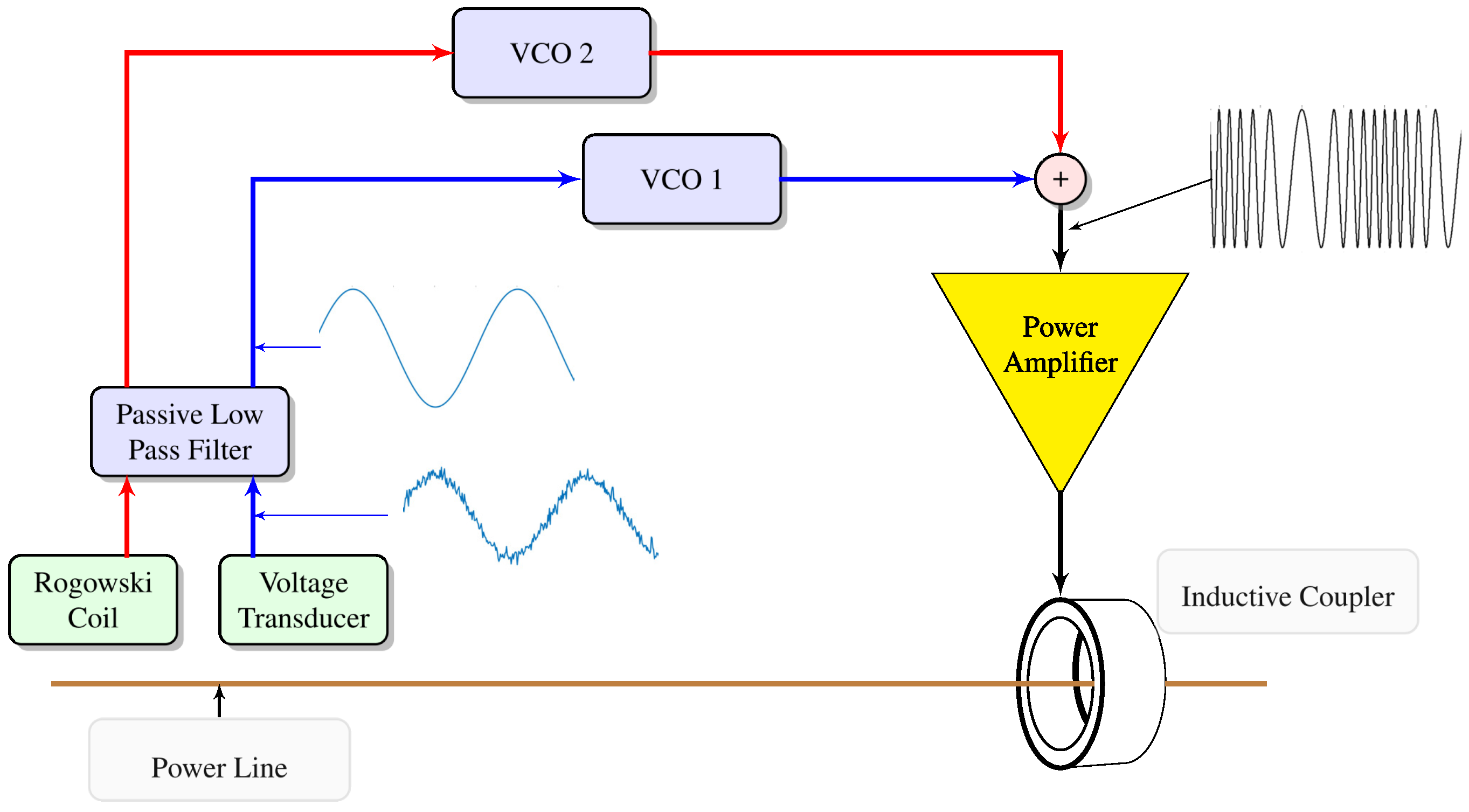
As an example, consider a signal with a centre frequency, , of 500 Hz and the signal varies to ±() Hz, where is the modulating signal, in this case the 50/60 Hz power frequency (and harmonics). This can be thought of as a type of frequency modulation because the amplitude of is encoded in the instantaneous frequency of the modulated waveform. More signals can be encoded by changing the centre frequency such that no two signals overlap. In this case, assigning an of 1500 Hz to another signal, and retaining the same sensitivity, would not lead to interference, though this assumes a bandlimited power frequency signal. A device capable of outputting a signal whose frequency is proportionate to the voltage of its input is a Voltage Controlled Oscillator (VCO). Such devices can be constructed and easily customised with readily available and inexpensive operational amplifiers and passive components, or off-the-shelf Integrated Circuits (ICs). Figure 1 shows a high level block diagram of the proposed transmitter architecture. The transmitter supports two channels so can convey both voltage and current information from a single observation point. Because the voltage and current are being modulated simultaneously, the transmitter is also capable of conveying the power factor angle.
It is assumed that there are many transmitters on a network, each occupying a set bandwidth. The high frequency signals from all transmitters are received by a single receiver. This work proposes communication from several monitoring positions on LV networks to a single observation point, most conveniently connected at the primary substation for the feeder. To keep costs to a minimum, we propose the use of the capacitive divider of the Voltage Detecting System (VDS), which are already installed in all major MV switchboards according to IEC 61243-5, for the receiver coupler. This method was recently presented in [24], with promising results in the kHz bandwidths. Using this method opens up the possibility of receiving the signal on the high voltage side of the transformer, avoiding the extra attenuation and frequency selectivity of the transformer.
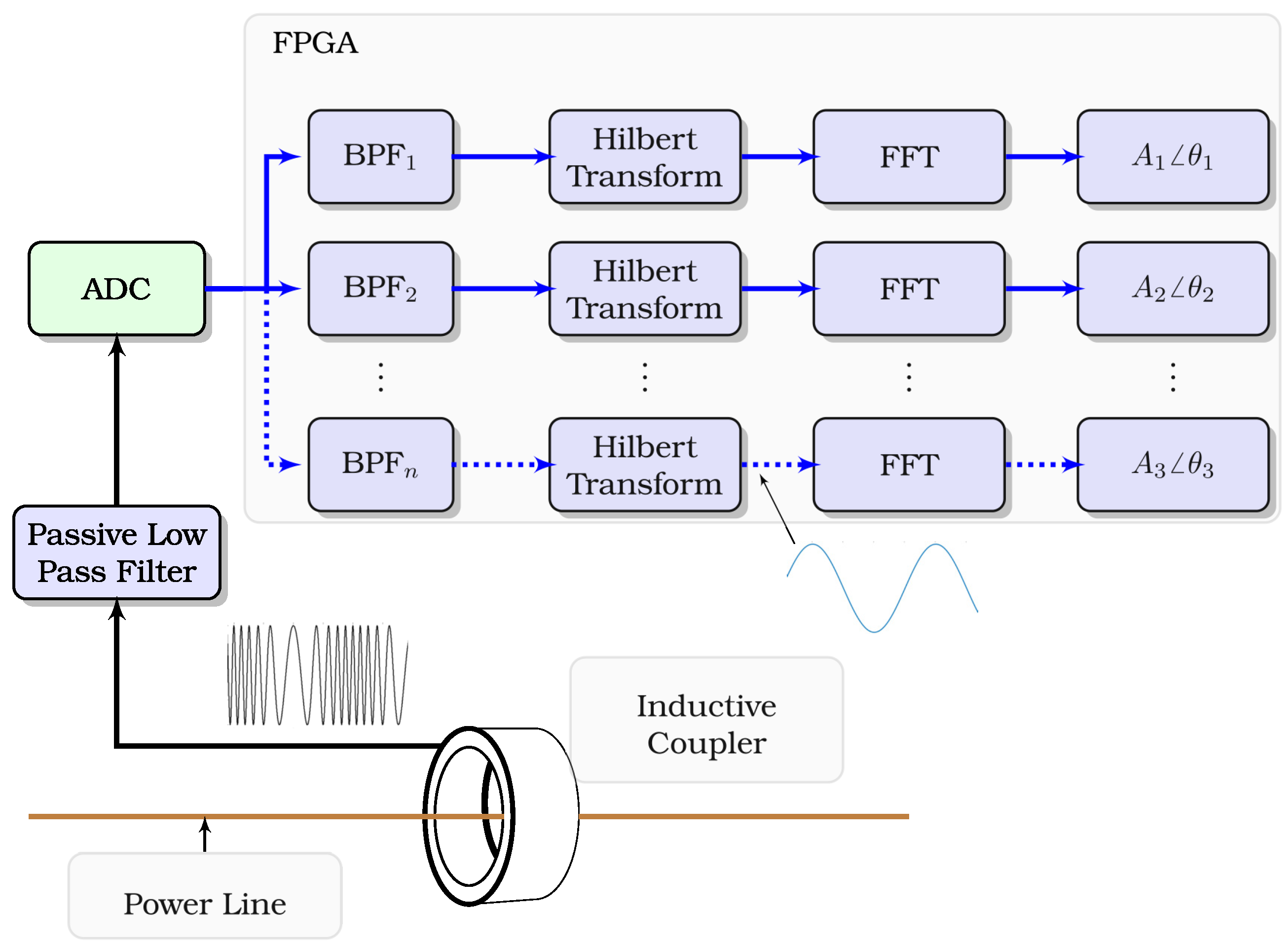
Following coupling, the received signal is sent to the receiver. Figure 2 shows a high level block diagram of the proposed receiver architecture. The first stage in the receiver is a bank of bandpass filters with high pass and low pass cut offs set to match the upper and lower frequencies of each of the transmitters.
To convert the frequency modulated high frequency signal back into the original power frequency signal that is modulating it, the Hilbert Transform (HT) is applied. The HT of a function is defined as:
where P represents the Cauchy principal value. Performing the HT on the signal allows it to be treated in the time domain as a rotating vector with instantaneous phase, and instantaneous amplitude, . In the time domain, this is given by:
The instantaneous phase is therefore given by:
Equation (5) can be realised in hardware efficiently using the CORDIC algorithm. Finally, the instantaneous frequency, , is the rate of change of phase with respect to time:
should be a replica of the original power frequency modulating the VCO transmitter. Further robustness has been achieved by using a final Fast Fourier Transform (FFT) block to determine the magnitude and phase of the power frequency and specified harmonics. If the receiver accepts signals from several transmitters simultaneously, the relative phase differences between the voltage and currents sharing the same transmitter location may be determined. Furthermore, the relative phase differences between transmitters at different locations may also be determined, providing the means to implement a real-time synchrophasor monitoring system without the requirement for time sychnronisation at the transmitters or any other form of communication.
The bandwidth occupied by each transmitter in the proposed scheme is of prime importance because it determines how many devices can operate simultaneously on a given network within a specified total bandwidth allocation. If it is assumed that the modulating signal, , is given by:
Then the instantaneous phase deviation is given by:
where the modulation index, is given by:
The FM modulated signal is therefore:
can alternatively be expressed as:
where is the Bessel function of the first kind. Here it can be seen that the spectrum of is that of an infinite sum of sinusoids with frequency increasing in multiples of , multiplied by the Bessel function. It is observed that the value dictates the strength and spread of the spectra around the centre frequency. Carson’s rule states that approximately 98% of the power in an FM signal lies within .
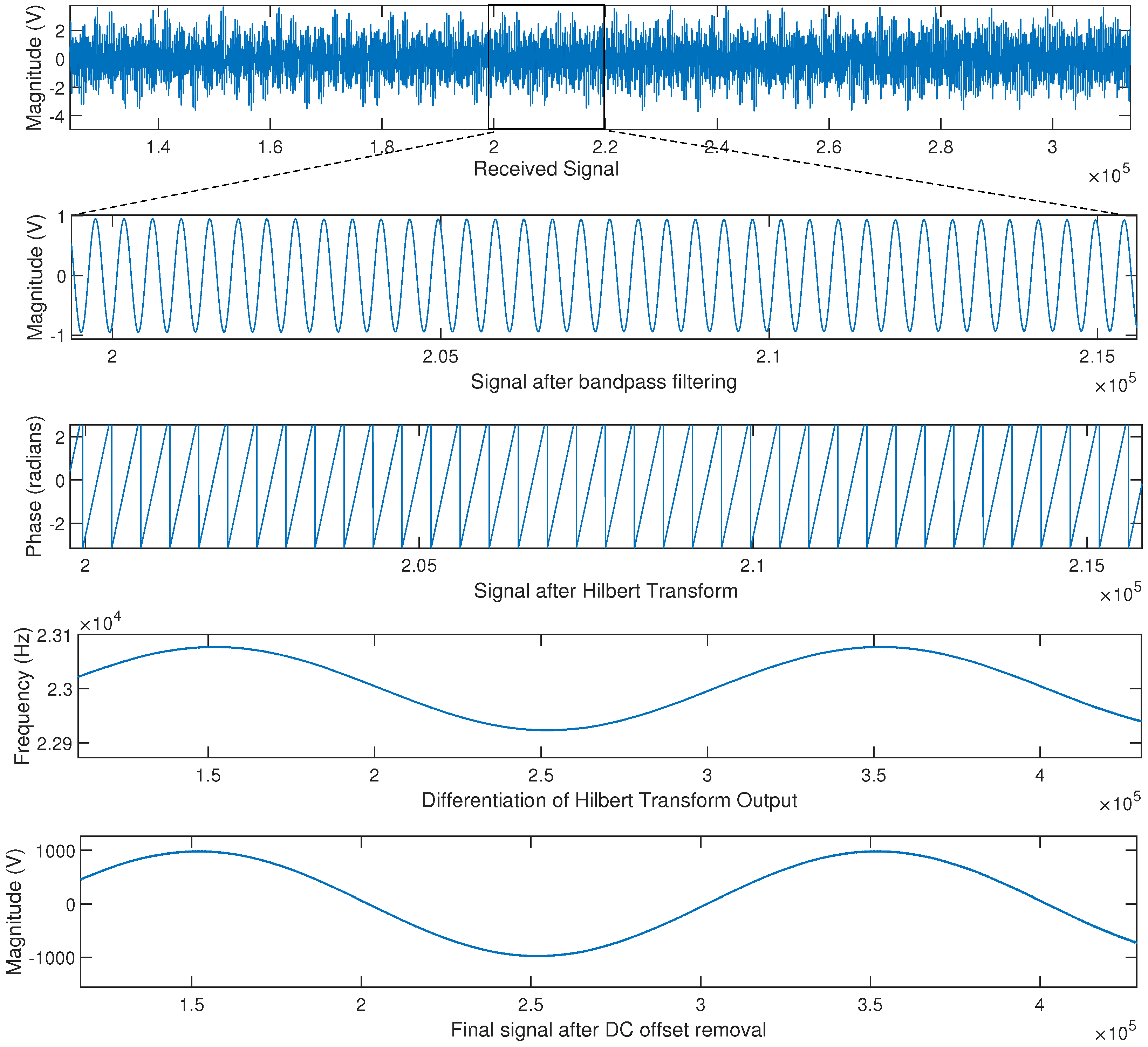
At the receiver, all that is known about the incoming signals is (1) The centre frequencies, and (2) The sensitivities, . Bandpass filtering isolates each of the n channels and the HT is performed separately and simultaneously on each. The result of the HT is the analytic signal, which may subsequently be converted to instantaneous phase; a sawtooth like waveform. The differential of the instantaneous phase yields the instantaneous frequency. If the offset is removed such that the waveform oscillates around 0 Hz rather than for that particular channel and scaled by the sensitivity factor, a replica of the power frequency waveform emerges. Figure 3 shows a representative set of signals at the receiver, here with an = 23 kHz.
FM has better resilience to noise and multipath interference than Amplitude Modulation. Such resilience may make FM a good candidate for applications on the power line channel, which are notorious for multipath interference and strong attenuation at particular regions of the spectrum [21]. In the past decade, narrowband PLC standards based on OFDM communication schemes have emerged. However, such systems require a local MODEM and may still be vulnerable to multipath effects in channels with large RMS delay spreads.
The proposed architectures for the transmitters and receivers have been tested using both Matlab-based simulation models and actual prototypes. For the latter, the transmitter has been realised using a commercially available VCO IC and readily available passive components. The receiver, which is more expensive to realise in hardware, utilises an FPGA in order to implement the necessary digital bandpass filters, HT, FFT and CORDIC algorithms.
3. Development of Simulation Scheme to Test Performance on a Typical MV/LV Feeder
As with any form of communication, the properties of the channel will play a crucial role in the performance of a given scheme. In this case, the power line itself is the channel. There are many studies in the literature which have attempted to characterise the power line channel from a communication perspective, with a high degree of frequency selectivity often cited as a particular challenge. To model the channel accurately, a similar methodology to that proposed in [21] is used. However, simulation of the proposed method also requires power frequency (and low harmonic) information, posing a difficulty since high frequency models for transformers, loads etc, are not appropriate for power frequency studies. Therefore, we propose the use of two parallel networks which run simultaneously in the same simulation—one for calculating the power frequency information and one for the high frequency communication study. Information from the power frequency study is recorded and passed to the transmitter model, which is implemented in the EMTP Models language. The VCO output of the transmitter model is coupled into the network. The whole process happens timestep by timestep in the simulation.
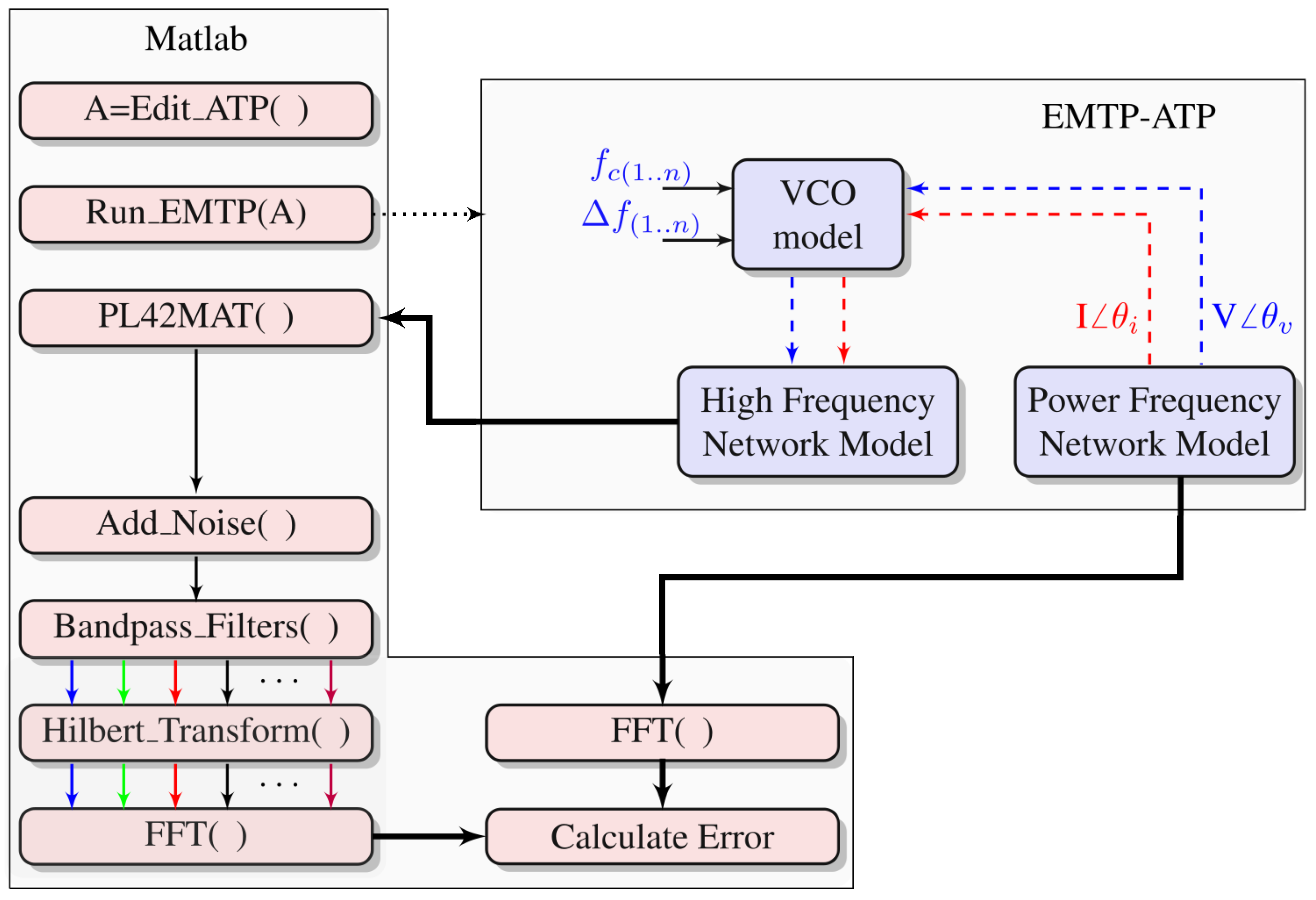
The simulation methodology used in this work is summarised in Figure 4. The Matlab domain is responsible for modelling the receiver and calculating the magnitude and phase errors based on comparisons between the actual voltage/currents from EMTP-ATP and the calculated values after propagation through the network and the receiver. The parallel networks within the EMTP-ATP domain is initiated from a DOS command within Matlab. Functions within Matlab have also been written to edit the VCO parameters of the transmitter models, such as centre frequency () and deviation (). Post-simulation, Matlab automatically converts the simulation results from .pl4 format to .MAT format, allowing automated processing.
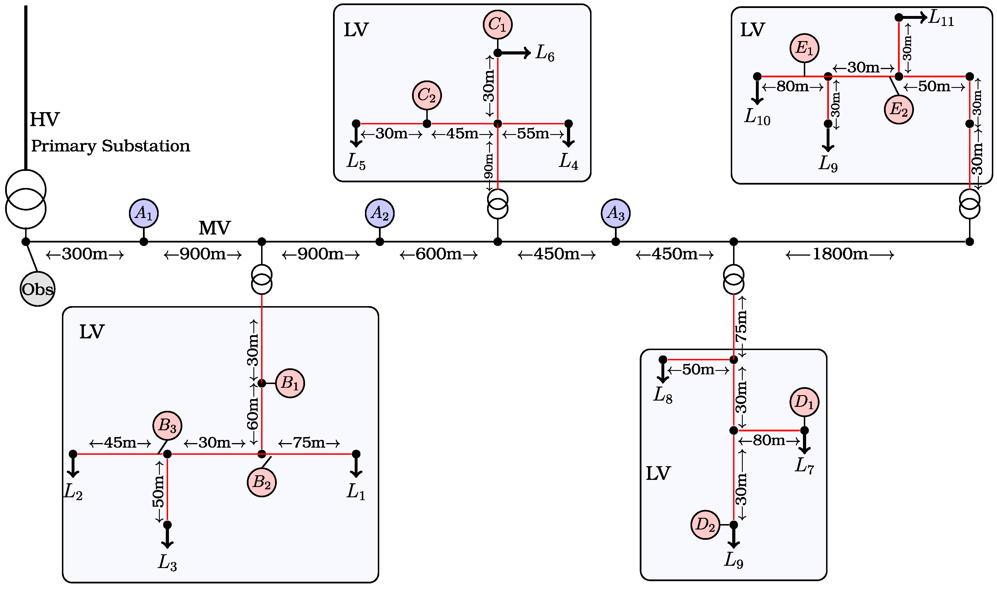
The simulation network modelled within EMTP-ATP is shown in Figure 5. It consists of a single primary substation. This has also been labelled as the observation point (“obs”) because the high frequency signals are taken from this position to be sent to the Matlab based receiver. The four three-phase LV feeders are modelled as underground cables (see Appendix A). The HV feeder runs at a nominal voltage of 10kV and is modelled as a three phase wood pole overhead line (also shown in Appendix A). In the power frequency simulation, loads (shown as to ) are represented as RLC elements.
3.1. EMTP-ATP Models
Within EMTP-ATP, two parallel networks are modelled and run simultaneously; one for the power frequency simulation and one for the high frequency simulation. Information from the power frequency solution is passed, during runtime, to VCO transmitter models, which are implemented within EMTP-ATP’s native models language (the code for the Model is shown in Appendix B). For example, considering the example network, the measured voltage and current waveforms from , , and , are passed to a series of VCO transmitter models. The output of the VCO models are immediately coupled back into the high frequency network at the same points.
In the high frequency models, extra care must be taken to ensure a representative channel model in the frequencies of interest. For the line and cable models, the JMarti frequency dependent line model is used [25]. For the transformers, Cataliotti’s medium frequency transformer model is used, which has been shown through empirical testing to perform well up to 100 kHz [26]. This has been implemented directly in the EMTP using lumped elements.
3.2. Implementation of the Receiver in Matlab
The receiver in the simulation studies is implemented within a Matlab script. To automate the process of performing the EMTP-ATP simulations, the same script is also capable of editing the ATP file (the text description of the circuit to be simulated) and running EMTP using a DOS command. Below is a brief description of each of the main functions within the Matlab script.
- Edit_ATP(): To automate and expedite the process of re-configuring the network between successive runs (i.e., to change the load conditions, Transmitter bandwidths, etc.), the ATP file, which contains a description of the circuit according to the EMTP rule book, is automatically re-written from within Matlab. In the code below, the edit function accepts two vectors; and f. is the vector of scaling factors (one for each VCO transmitter in the EMTP network). f is the vector of centre frequencies for each VCO transmitter. A DOS command run within Matlab is used to copy a fresh version of the .atp file for each run of the simulation. This is followed by the edit function, which contains code to edit the atp file by printing the and f values at the appropriate position.

- Run_EMTP(): The EMTP-ATP is run using dos command from within Matlab.

- PL42MAT(): The EMTP-ATP simulation results are by default in PL4 format. PL42MAT() converts the PL4 data format to the .MAT data format for subsequent processing in the Matlab environment.

- Add_Noise(): This is an optional function which adds a specified amount of AWGN noise to the received signal, enabling Monte Carlo type studies.
- Bandpass_Filters(): A bank of configurable bandpass filters were used to split the incoming signal by frequency to isolate the signal sent by each of the n transmitters.

- Hilbert_Transform(): Matlab’s native Hilbert Transform function is performed on each of the n incoming signals following separation by frequency. The subsequent waveform is a replica of the original power frequency signal centred around . Subtracting brings the signal back down to a centre frequency of DC.

- FFT(): Following the Hilbert Transform, each of the n signals should resemble the original power frequency signal at the transmitter. A final FFT is performed on each of the n incoming signals to conveniently calculate the amplitude and phase of the power frequency and, optionally, the harmonics.
- Calculate_Error(): An error function is used to compare the receive values with the actual values.

4. Simulation Results
4.1. Channel Properties
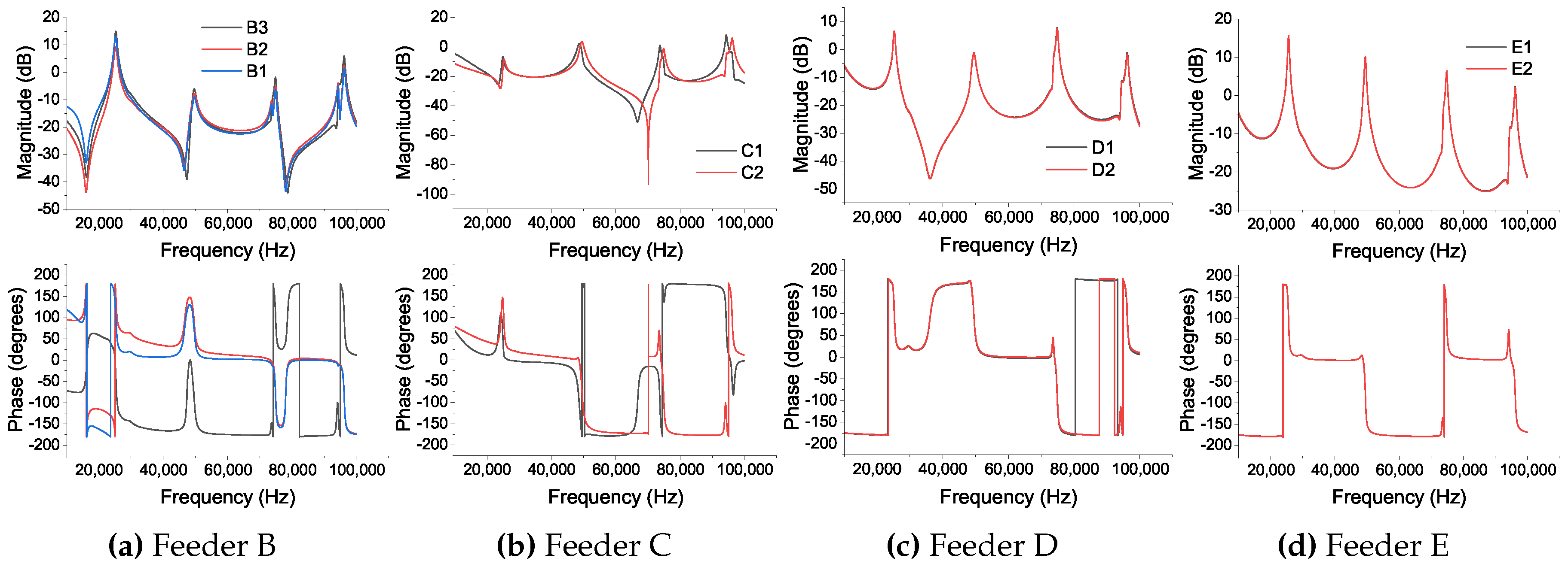
The channel response separating the transmitter(s) and receiver determines the attenuation and phase shift experienced by the signal as a function of frequency. It is well known, both from simulation [21] and empirical studies [27] that the power line channel is highly frequency selective, leading to peaks and troughs in attenuation and sharp changes in phase over relatively narrow bandwidths. In multicarrier communication schemes, these abrupt changes in phase over relatively narrow bandwidths result in impairment of the received BER, especially in cases where the information is encoded as the phase difference between adjacent subcarriers. The associated phenomena of strong dips in the magnitude response also impairs the BER due to the reduction in SNR. The magnitude and phase responses are calculated using the frequency scan function in EMTP-ATP. The results for channels in Feeders B, C and D are shown in Figure 6.
It is observed that the channel responses between the observation point and transmitters on the same feeder are broadly similar, sharing the same peaks and troughs, though some phase differences are apparent. Across all channel responses, there are frequencies exhibiting high attenuation and sharp phase discontinuities. Transmitting at these frequencies may reduce the received power well below the noise floor and the erratic phase response may affect the quality of the FM signal. It is interesting to note that the different feeders share frequency regions which are particularly hostile to communication, for example, all feeders exhibit significant phase non-linearities at 75kHz. Such a result, if replicated on real networks, may open up the possibility of only having to perform a single channel survey to determine which frequencies are best avoided for that particular network.
4.2. Performance over AWGN Channel
Monte-carlo simulations were performed to assess the performance of the proposed scheme when subjected to Additive White Gaussian Noise (AWGN). A carrier frequency of 10 kHz was chosen, with a variable VCO bandwidth modulating a 50 Hz input signal. Although the overall sampling rate is set at 10 MHz, bandpass filtering is performed at a lower sampling rate (200 kHz) to ease the performance requirements. The bandpass filter is designed to provide a bandpass region of approximately twice the used VCO bandwidth and a steepness of 0.98 (using Matlab’s IIR design function filtfilt()). Noise is added to the modulated signal prior to filtering and a final FFT stage is incorporated to measure the magnitude of the 50 Hz component. The simulation results are shown in Figure 7. It is observed that the error variance, defined here as the variance of the error between the magnitude of the actual and reconstructed 50 Hz signal, drops as the used VCO bandwidth increases. Similarly, the error variance improves with increased SNR, with an order of magnitude drop observed for a 10 dB improvement in SNR. Clearly, there is a trade-off between the occupied bandwidth per transmitter and error variance—i.e., error variance may be sacrificed for reduced bandwidth and vice-versa.
4.3. Performance on the EMTP/ATP Network
4.3.1. System Design
Using the methodology outlined in Section 3, the performance of the proposed scheme is assessed on the representative MV/LV network shown in Figure 5. The system is designed such that each transmitter has a maximum frequency deviation, , of 78.5 Hz (equating to rated voltage of 1000 V or rated current of 1000 A), corresponding to a modulation index, of approximately 1.6. The occupied bandwidth of each channel is, according to Carson’s approximation, a maximum of 300 Hz at rated values. Each channel is allocated 4 kHz of bandwidth, with the first channel allocated to VB1 (Voltage from B1) at = 15 kHz, the second allocated to IB1 (current from B1) at = 19 kHz, and so on. The total system bandwidth for all transmitters extends up to = 83 kHz. A bank of bandpass filters with −3 dB bandwidths of ±550 Hz around each is used, as specified in Section 3.2.
4.3.2. General Performance
Table 1 shows simulation results for arbitrary loads conditions and a CNR of 40 dB.
In general, Table 1 reports good performance for magnitude and a mixed accuracy for phase. The worst channel in terms of magnitude and phase is IE1, which may be explained by considering the affect of the channel response (Figure 6d) at the carrier frequency of interest, i.e., 75 kHz. As already mentioned, there is a relatively low attenuation and a sharp discontinuity in the phase response in this particular channel. The effect of the channel on the accuracy of the magnitude is less pronounced than for phase.
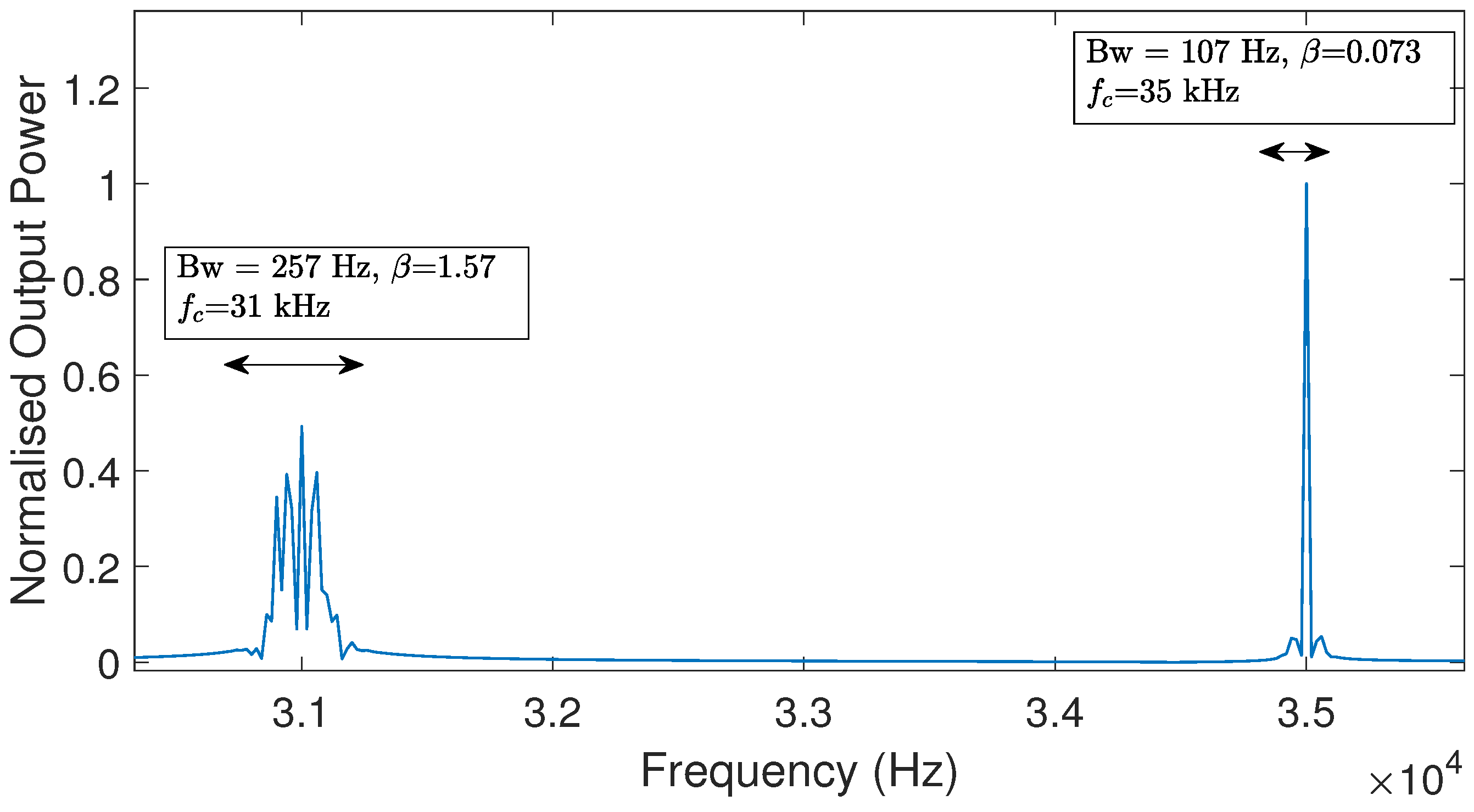
It should also be noted from Table 1 that when the sensitivity is fixed, the occupied bandwidth per channel will be proportionate to the magnitude of the measured signal. For example, consider position B3, which measures an rms voltage of 982.59 V and an rms current of 98.22 V. This results in a modulation index, of 1.544 and 0.154, respectively. Figure 8 shows the spectra of these two signals as they appear on the output of the transmitter (i.e., they have not yet propagated through the channel). The practical consequence of this is twofold: (1) For fixed sensitivities, large voltage and current signals may push the bandwidth beyond the allocated limits, (2) In the case of small voltages and currents, narrower bandwidths, i.e., low modulation indices, will result in a poorer SNR at the receiver.
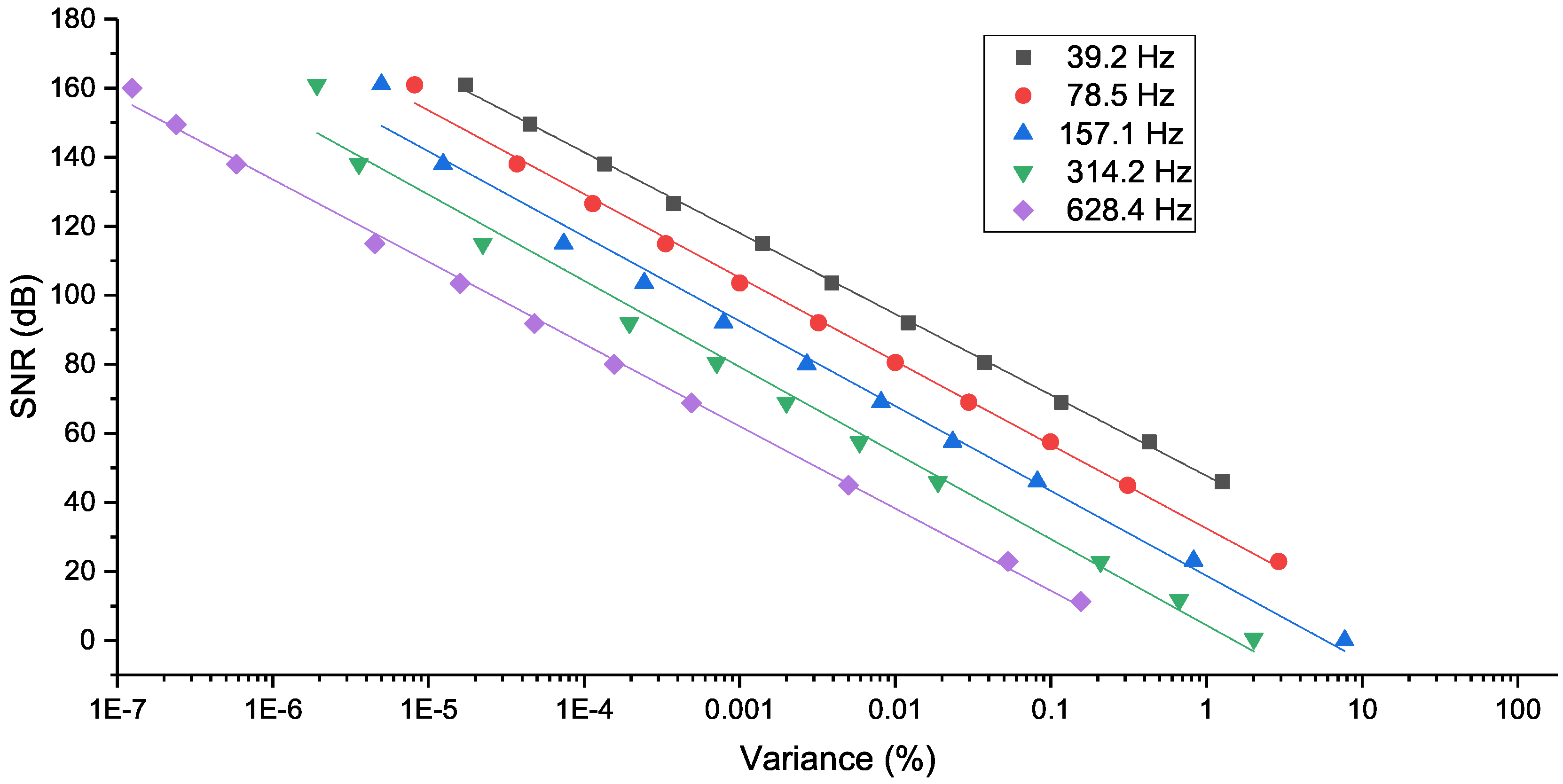
Figure 9 shows the correlation between SNR and variance (for magnitude) for transmission from all possible transmitters on all feeders. Under such circumstances, the performance is almost identical to that of the AWGN channel, indicating that the frequency selectivity channel is not impairing the quality of communication beyond the immediate penalty paid for lower SNRs. This is a marked advantage over digital communication systems which are vulnerable to intersymbol interference on highly frequency selective channels such as those associated with MV networks.
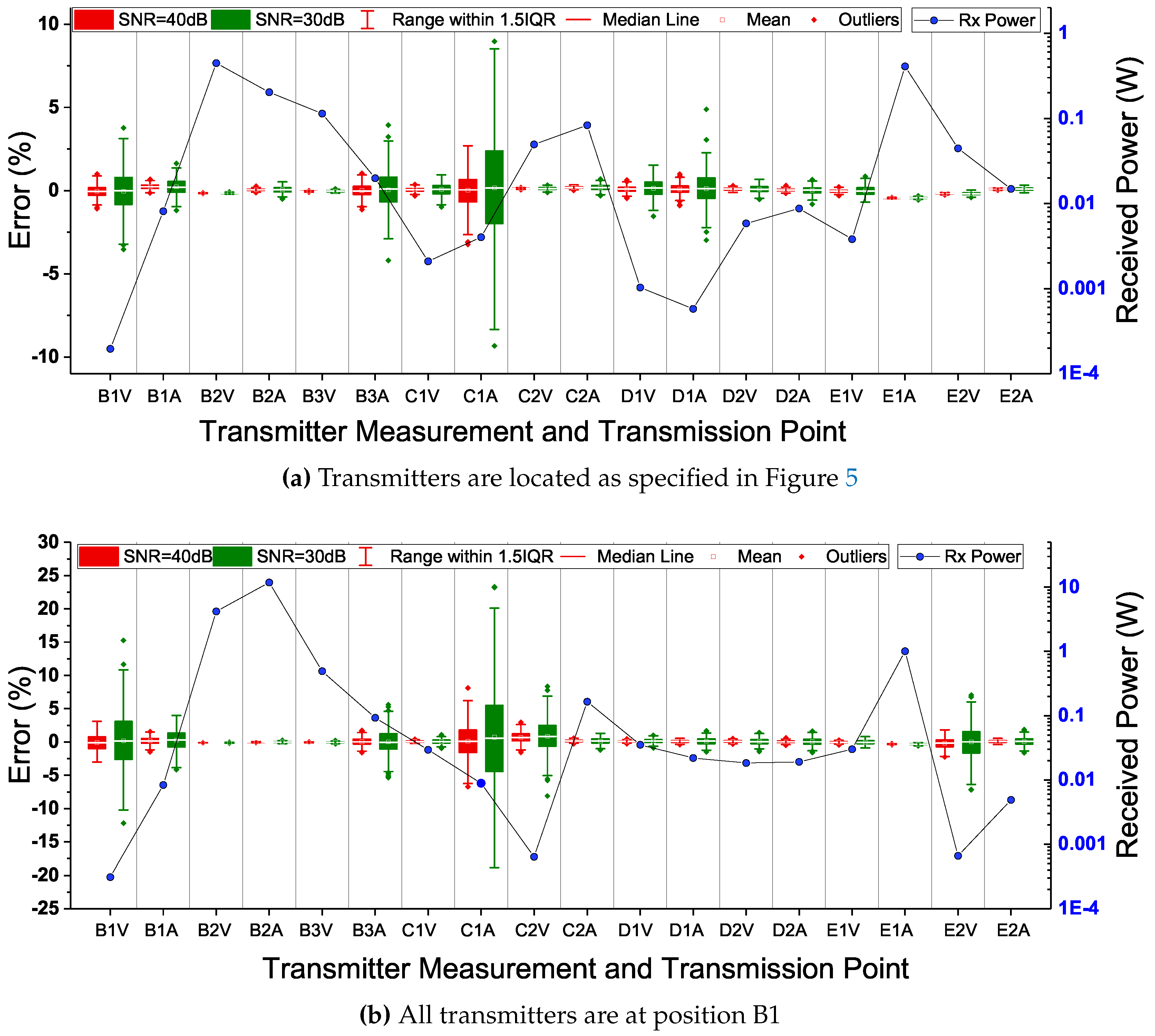
To further investigate the quality of communication as a function of transmitter position and channel characteristic, Figure 10 shows box-whisker plots of error variance as a function of transmitter location. In Figure 10a, each transmitter monitors the voltage and current at their respective location and subsequently transmits from that location.
In Figure 10 it is assumed that the transmitters are all located at node B1 (but they are nonetheless monitoring the indicated point). This is to make it easier to visualise the affect of the channel.
4.3.3. Phase Measurements
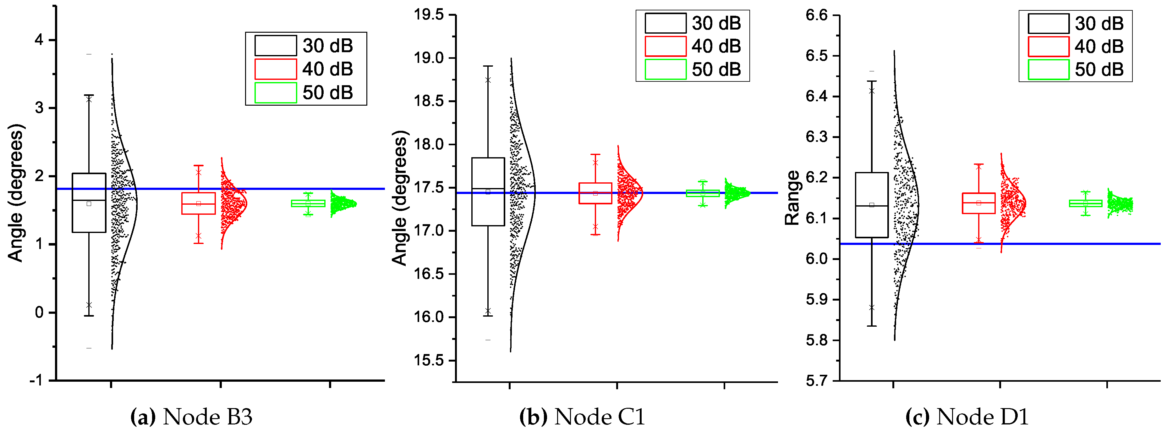
The output of the second FFT within each channel of the receiver (as outlined in Figure 2) outputs complex data from which the relative phase between parallel voltage and current measurements can be determined. The phase difference between voltage and current from the same node is the power factor angle, . It has been observed that the phase angle, as measured at the transmitter, is preserved at the receiver. Table 1 has shown that a reasonable approximation of is possible using the proposed method, though deterioration of performance is observed on selected channels due to low SNR caused by deep fades in the magnitude response. Figure 11 shows Box-whisker plots of as estimated by the receiver versus actual values as measured directly at the node, where the horizontal blue line represents the actual value. In terms of variance (that is, scatter around the distribution’s mean value), performance tends to improve significantly with an order of magnitude improvement in CNR. However, an offset is occasionally present which displaces the received distribution’s means by a small amount.
4.3.4. Harmonic Measurements
An interesting attribute of the proposed method is the ability to estimate harmonic information. Doing so will come at the expense of an increased transmission bandwidth. Equation (8), which shows the instantaneous phase deviation for a single tone, can be generalised for n tones:
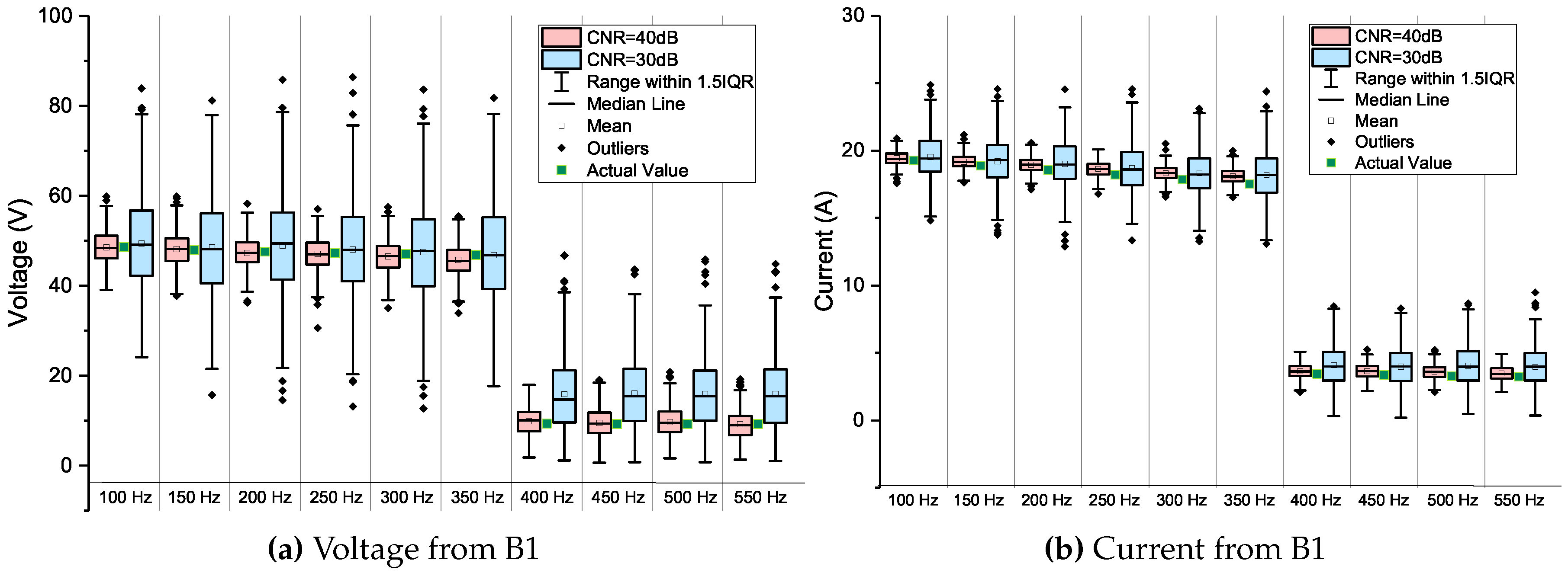
Each of the n harmonics will have its own modulation index, , but can nonetheless be scaled similarly to the fundamental at the power frequency. To test the harmonic measurement capability of the proposed system, the harmonic voltage source (HFS_Sour) from within EMTP-ATP is used, and the first six harmonics (100 Hz → 350 Hz) are set to an amplitude of of the fundamental. Harmonics 7 to 10 (400 Hz → 550 Hz) are set to an amplitude of of the fundamental. Figure 12 shows a representative set of measurements of harmonic information taken from the receiver associated with the transmitter at node B1.
Figure 12 shows that harmonic information is indeed being transmitted and received to a good accuracy, though accuracy improves significantly with improved CNR.
4.3.5. Synchrophasor Retrieval
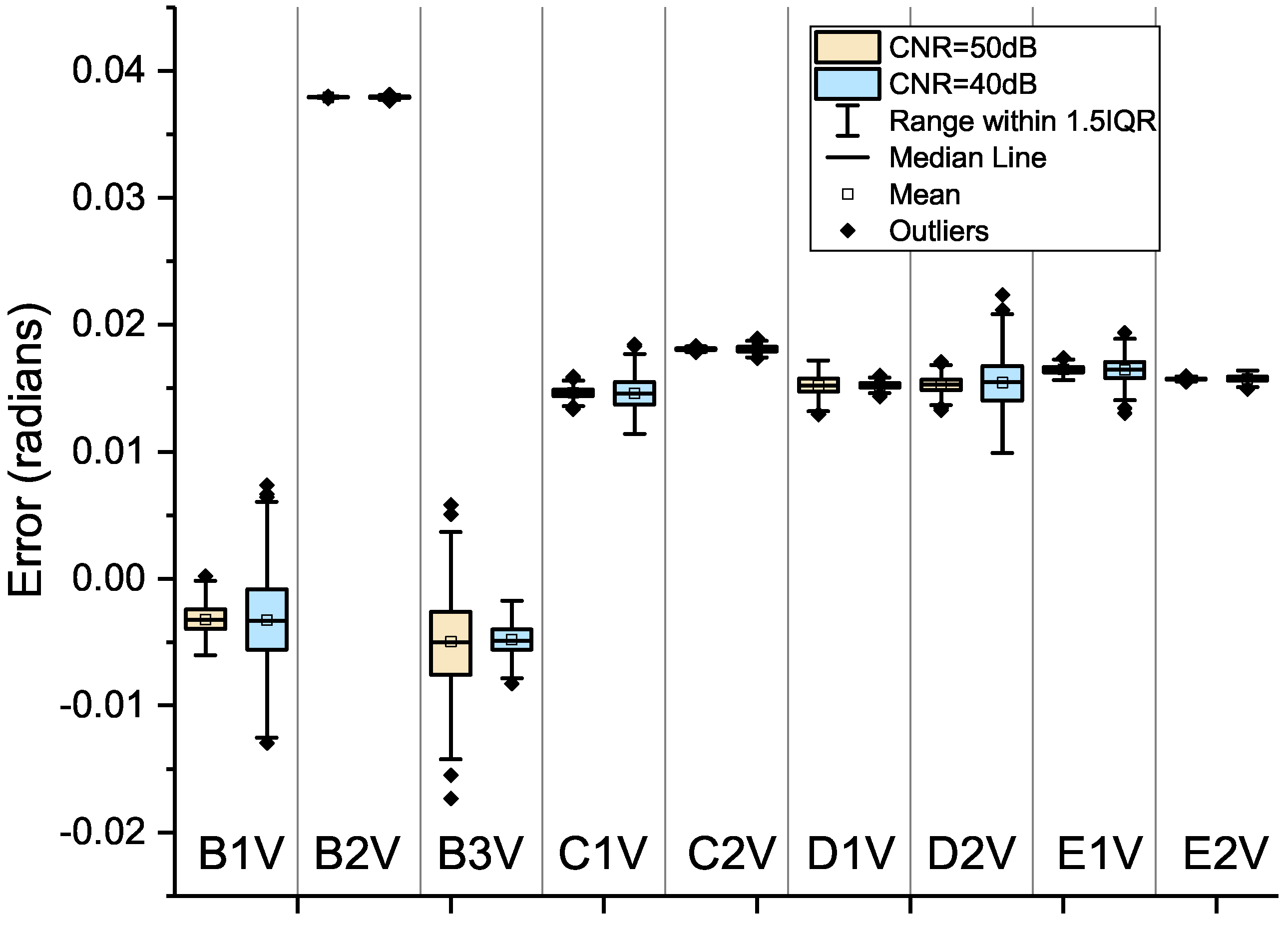
An advantage of the proposed method is the lack of the requirement for a GPS synchronised clock at each of the transmitter locations, as is required by traditional PMU installations. Since the voltage and current waveforms are immediately frequency modulated and re-injected back into the network, then immediately processed by the receiver, the phase differences between nodes on the grid may be preserved, fulfilling one of the requirements of a synchrophasor measurement system. The difference in the travel times between each transmitter and the receiver may differ, but this is likely to be negligible relative to the period of the fundamental frequency, even for large networks. Figure 13 shows box-whisker plots of the error between the actual phase of the nodal voltage and the received phase using the proposed method. There appears to be a small offset in all of nodes. The worst error is observed for node B2, where a 0.04 radians (2.3) error was recorded. It is interesting to note that although the offset is relatively high, the range around the mean is small. This result could be explained with reference to Figure 6a, which shows a prominent peak in the magnitude at around 23kHz, which coincides with the centre frequency of transmitter VB2. At the same frequency, there is a sharp phase discontinuity. This implies that the phase response of the channel is more important than the magnitude response when considering the accuracy of the method.
5. Prototype Build
5.1. Build of VCO Transmitter
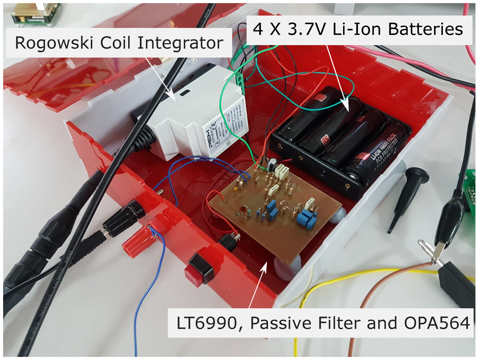
An important feature of the transmitter architecture shown in Figure 1 is that it requires no local intelligence (i.e., microcontroller), and can operate from relatively inexpensive parts (VCO, passive filter, power amplifier, battery, voltage/current transducers and inductive coupler).
The VCO is realised using the LTC6990, which operates within a frequency range of 488 Hz–2 MHz (programmable) with a VCO bandwidth of greater than 300 kHz at 1 MHz. The LTC6990’s produces a square wave with a 50% duty cycle at a frequency which is proportionate to the input voltage. The output square wave is low pass filtered to produce a sinusoidal wave.
The input to the LTC6990 is derived from the power frequency voltage/current transducer. In this prototype, a rogowski coil (PEM manufactured RCTi/250/1/700/BC with a full scale output of 5 Vrms at 250 A, a phase shift of 0.9 ± 0.1, −3 dB bandwidth of 0.6 Hz to 600 kHz and an accuracy of 1%) is used to measure current and a voltage divider circuit is used to measure voltage.
To drive the output of the VCO into the power line, the OPA564 power Operational Amplifier (Op-Amp), which is capable of delivering 1.5 A into a reactive load at a gain-product bandwidth of 17 MHz, is used. This drives a current into an inductive coupler which has a mutual inductance of approximately 5 nH with the power line. Note that for LV (<400 V) injection, it may be more practical and cost-effective to use a coupling capacitor.
5.2. Build of FPGA-Based Receiver
The receiver’s role in the proposed method is to (a) Separate the received signal in frequency, thereby isolating the FM signal from each of the transmitters on the given network into n channels, (b) Perform the Hilbert Transform on each of the n channels. The incoming signal is first sampled using the LTC2308 Analog to Digital Converter (ADC) at a rate of 102.4 kHz. Subsequent bandpass filtering separates the signal into each of its n channels. This can be acheived using a bank of FIR digital filters.
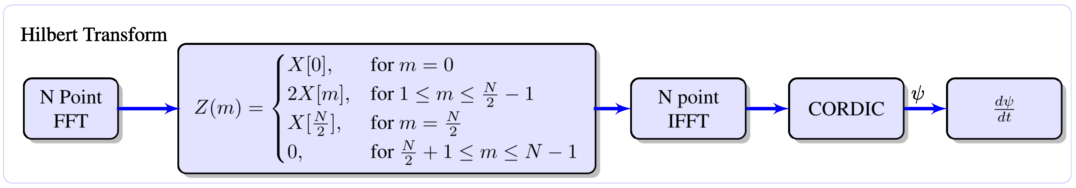
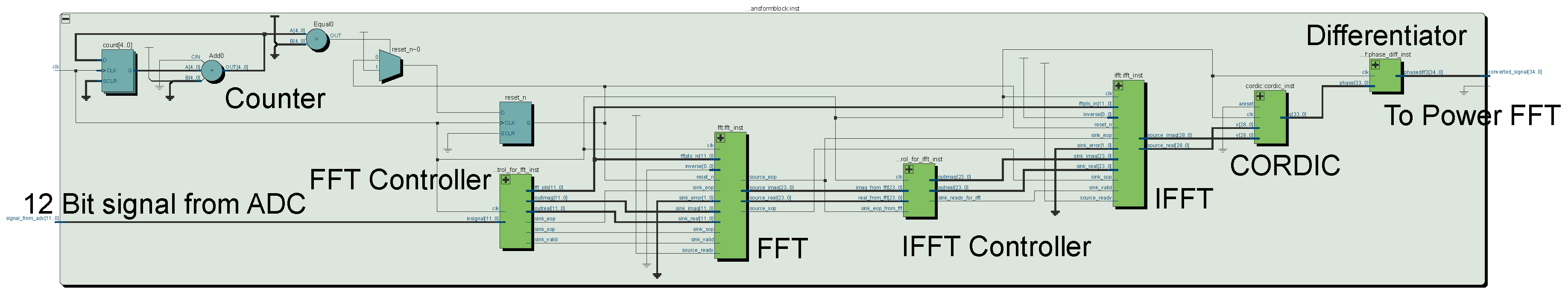
Implementation of the Hilbert Transform has been achieved in FPGA hardware using a 2048 point FFT-IFFT pair. As indicated in Figure 2, the output of the FFT is manipulated to derive the one-sided analytic signal by setting the negative side of the spectrum to zero. This signal is subsequently processed by the IFFT, whose output is the analytic signal. The real and imaginary outputs of the IFFT are converted to phase using a CORDIC algorithm set to Atan2 mode. The output of the CORDIC algorithm is the instantaneous phase of the FM signal entering the channel. Differentiating the phase with respect to time leads to the instantaneous frequency. A high level block diagram of the HT is shown in Figure 16.
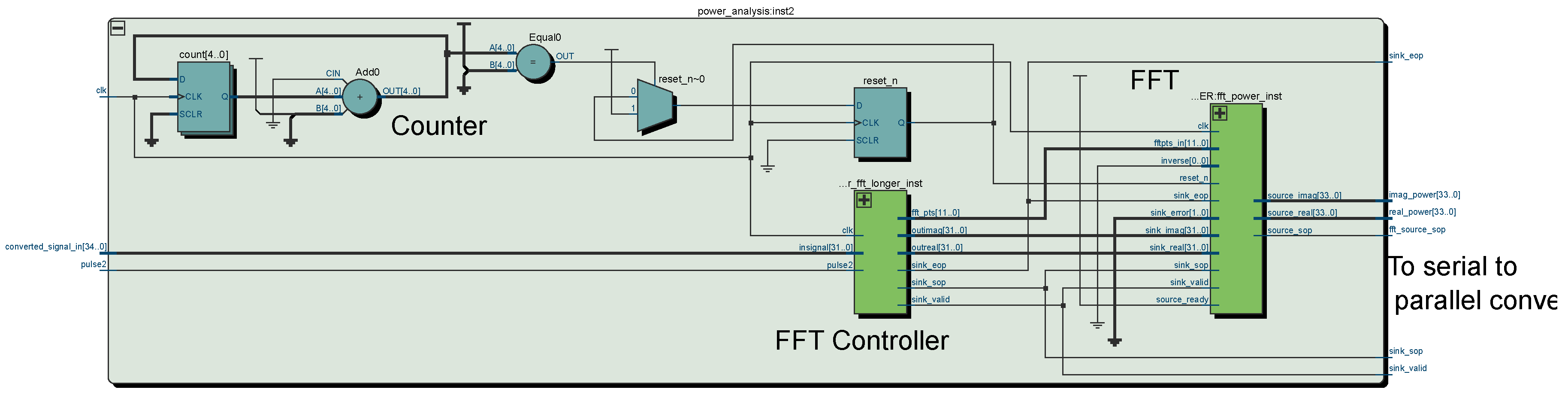
In FPGA hardware, simple numerical differentiation (with additional logic to deal with wrapping) is used to calculate from . In this case, will be a reconstruction of the original power frequency waveform entering the VCO at the respective transmitter. To increase robustness against noise, the output of the CORDIC algorithm is processed by another 2048 point FFT to determine: (1) The magnitude and phase of the fundamental frequency (the first coefficient above DC), (2) The magnitude and phase of the harmonics. Following this procedure on all n channels yields n magnitudes and phases which may be compared. Furthermore, if the windows of the final FFTs are synchronised to a known time, the process can yield synchrophasor estimations. In practice, this can be enabled by locking the FFT “start of packet” (a one pulse flag which signals the first sample into the FFT block) to a GPS clock local to the receiver. This GPS clock is derived from a Motorola M12M Oncore timing receiver.
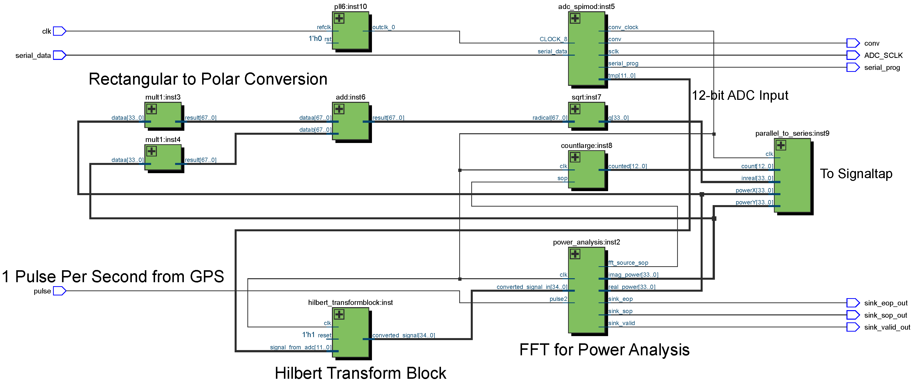
The overall FPGA design is summarised by the Register Transfer Level (RTL) representation in Figure 17, which has been taken from Quartus post-compilation. The RTL representations of the two main blocks in this design; The “Hilbert Transform” and “FFT for Power Analysis” blocks, are shown in Figure 18 and Figure 19. Interrogation of the relevant signals is achieved using the Signaltap tool within Quartus, which is a real-time system-level debugging tool allowing the user to view and save signals inside the FPGA. Table 2 summarises the resource utilisation of the FPGA.
6. Experimental Results
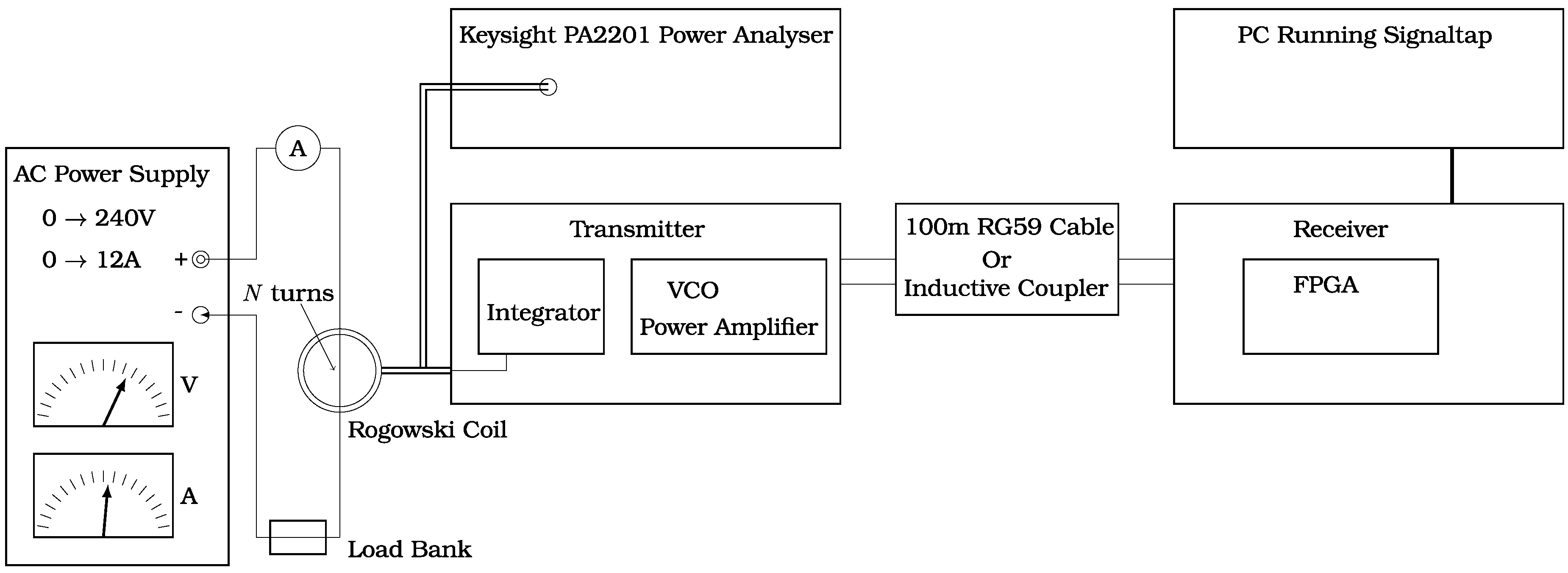
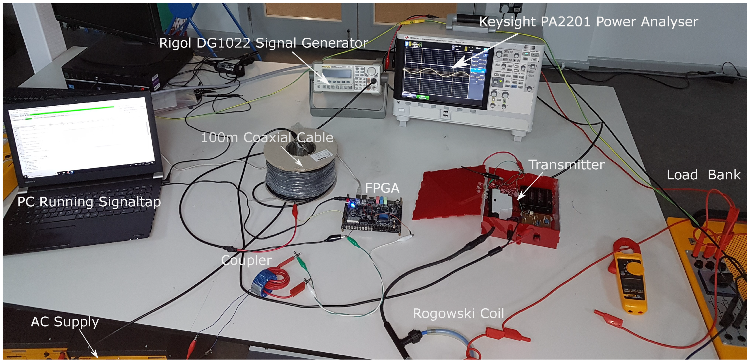
Figure 20 and Figure 21 shows a block schematic of the experimental setup used to determine the performance of the proposed method. Initially, a single transmitter (single channel) is considered, meaning only magnitude can be assessed at this time. The test setup is comprised of an AC power supply capable of outputting 12 A at 240 V and a variable resistive load bank to produce a variable current at mains frequencies (50 Hz in the United Kingdom). A rogowski coil (as described in Section 5.1) is used as the transducer. To increase the current, the current carrying conductor is wrapped around the rogowski coil 10 times, increasing the effective range of current to 0→120 A. The output of the rogowski coil is sent into both the Keysight PA2201 Power Analyser (for measurement) and the transmitter, for frequency modulation and subsequent transmission.
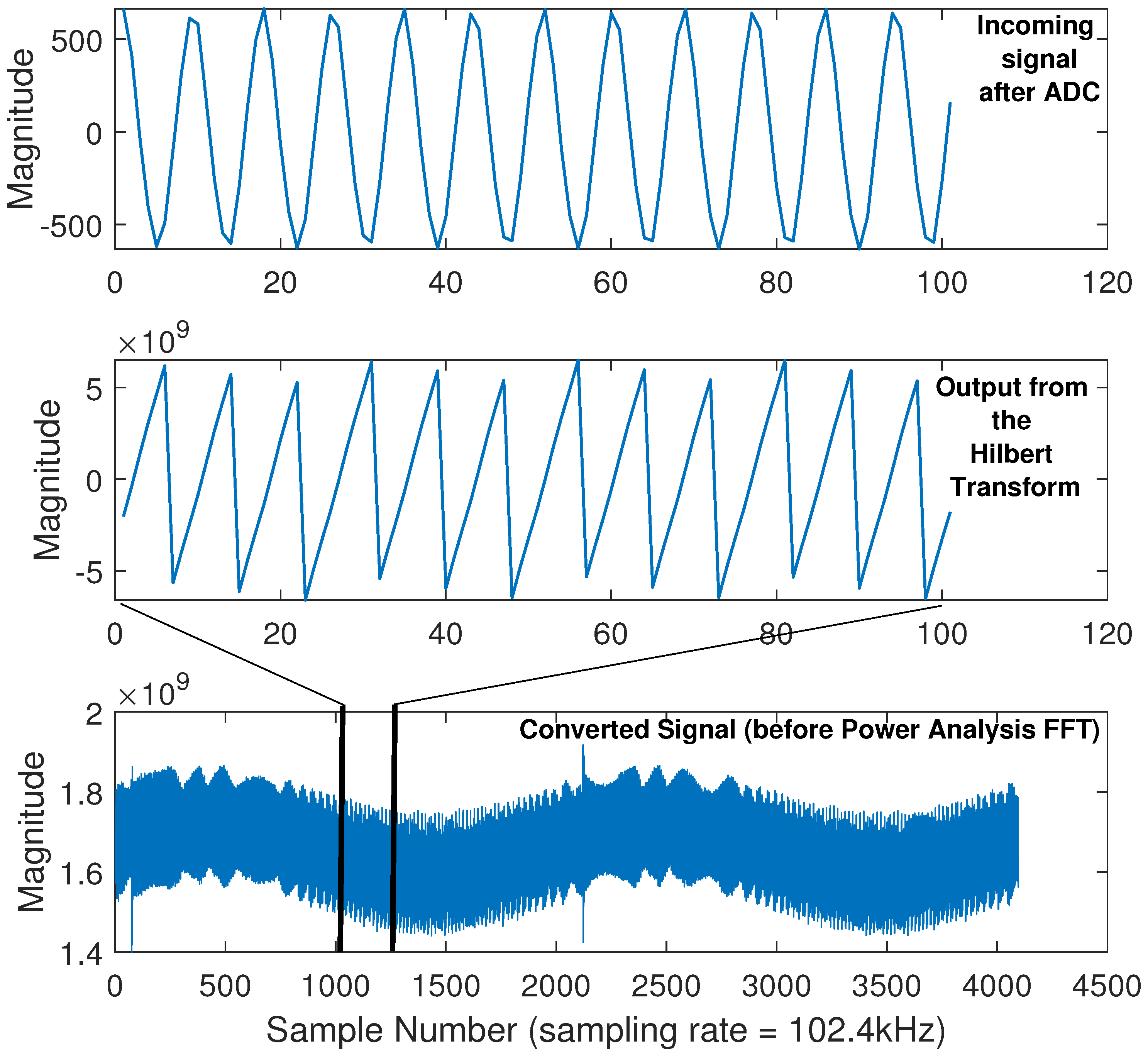
Figure 22 shows typical waveforms obtained from signaltap during the course of the experimental testing. Note that a zoomed in view is displayed in the top two graphs in order to preserve detail, but a full cycle of 50 Hz is displayed below (“converted signal”). A notable feature of these results is the high degree of noise in the converted signal (bottom plot). This high level of noise is due the method of differentiation used in the FPGA (simple numerical differentiation). However, the accuracy of the method is dependent more on the fundamental 50 Hz frequency, which becomes apparent after performing the power analysis FFT. Future work will examine more effective methods of differentiation.
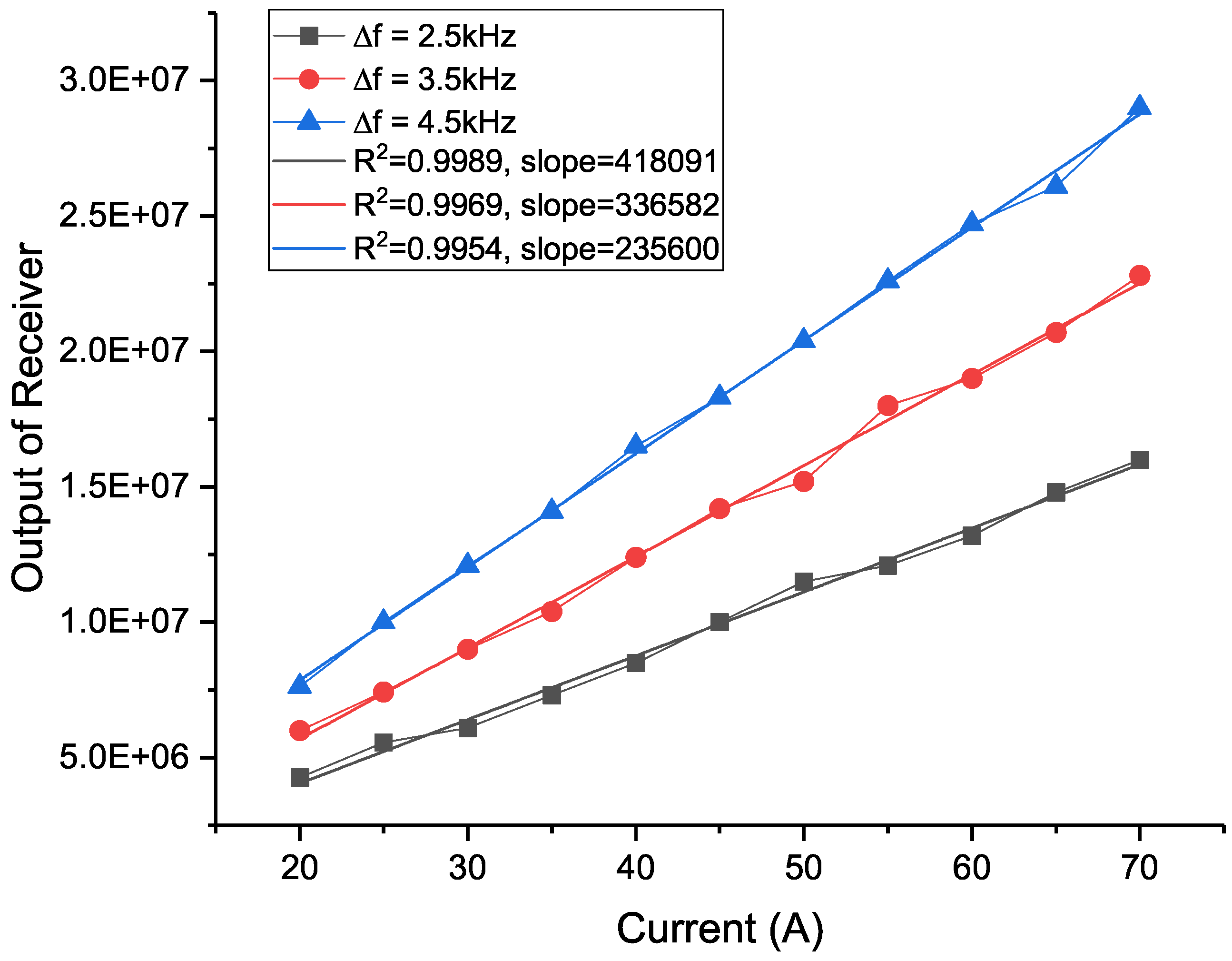
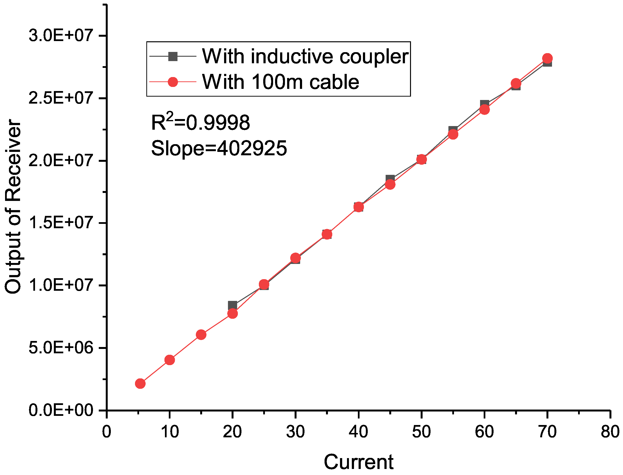
Prior to the experimental testing, the receiver was injected with an FM signal generated by a Rigol DG1022 signal generator (which is used as a comparison/benchmark against which the real transmitter can be tested). For this test, the magnitude and frequency of the modulated signal was set to 830 mV and 13 kHz respectively, with the modulating signal derived from the rogowski coil, as specified in Figure 20. Figure 23 displays the results for frequency deviations of 4.5 kHz, 3.5 kHz and 2.5 kHz. In all three situations, the relationship between the measured current and the output from the receiver follows a linear relationship, though the slope is different because the effective sensitivity, is different in each case. Figure 24 shows the test results for the two experimental setups of Figure 20, i.e., one case which uses an inductive coupler to link the transmitter and receiver, and the second case which uses a 100 m coaxial cable transmission line. It is observed that both cases result in the same output, indicating that the 100 m line has had no observable adverse effect on the signal. This matches the observation from the simulations, i.e., the channel itself has little effect on the quality of communication.
7. Practical Considerations and Future Work
The proposed method is well suited to applications in rural and semi-rural distribution grids where conventional monitoring technology, and the associated communication infratructure, is not deemed economically justifiable. The method depends on availability of bandwidth in the Cenelec range of frequencies, which is also sometimes occupied by narrowband PLC systems. Future work will examine ways in which these two technologies may co-exist. Power requirements for the proposed method are expected to be supplied directly from the LV network, so an additional AC to DC power supply will be required. An option which has not been looked at in this paper, but may nonetheless be attractive, is to use the proposed method for monitoring and communication directly on the MV side of the network. A combined monitoring and communication device could be built using only an inductive coupler. Powering such a system would necessitate some form of energy harvesting and the power consumption of the device could be significantly reduced by only transmitting for a particular portion of time. Using the enable pins on the LTC6990 and OPA564, in combination with a timer circuit (such as the 555 timer set to a particular duty cycle) would provide a practical way to do this. The developed prototypes will be further tested to examine whether synchrophasor measurements can be carried out in practice, as indicated by the simulations. In addition to voltage, current and phase, the proposed method may also be used to communicate condition monitoring information, e.g., real-time conductor temperatures or leakage current [28]. It may also be deployed to support multi-ended fault location algorithms, for example [29,30].
8. Conclusions
This paper presents a new, low-cost technique for monitoring voltage, current and synchronised phase angles in distribution networks. Unlike traditional PMU systems, the proposed system requires no time-synchronisation at the transmitters and can be constructed using readily available electronics. Furthermore, the communication requirements are inherently met by the nature of the system. The method is based on FM of the monitored fundamental power frequency signals (and low harmonics) and immediate injection of the modulated signal into the network, where it can propagate to a central point. It has been observed through Matlab and EMTP-ATP simulations that the method is capable of not only conveying the magnitude of the monitored signals, but also the phase differences, perhaps making possible a low-cost synchrophasor system. To demonstrate the practicality of the system, a working prototype has been built which has been observed to successfully convey the magnitude of a measured current in laboratory conditions. The viability of the method will be further explored in larger scale trials in the near future.
Author Contributions
S.R. and G.T. conceived of the methodology. S.R. performed the simulations and wrote the manuscript. G.T. designed and constructed the transmitter circuitry. S.R. and G.T. designed and built the FPGA receiver design. S.R., G.T. and A.H. were responsible for initial discussions of the idea, discussion and analysis of results and reviewing of the manuscript.
Funding
The authors would like to thank the Engineering and Physical Sciences Research Council (EPSRC) for the financial support of this research programme through grant number EP/F037686/1: “Power Network Research Academy” in collaboration with four major UK electricity utilities: National Grid plc., Scottish and Southern Energy plc. (SSE), UK Power Networks (UKPN) and Western Power Distribution (WPD). The authors would also like to acknowledge the financial support of the “student sensors competition” which is part of the DEDUCE project.
Conflicts of Interest
The authors declare no conflict of interest.
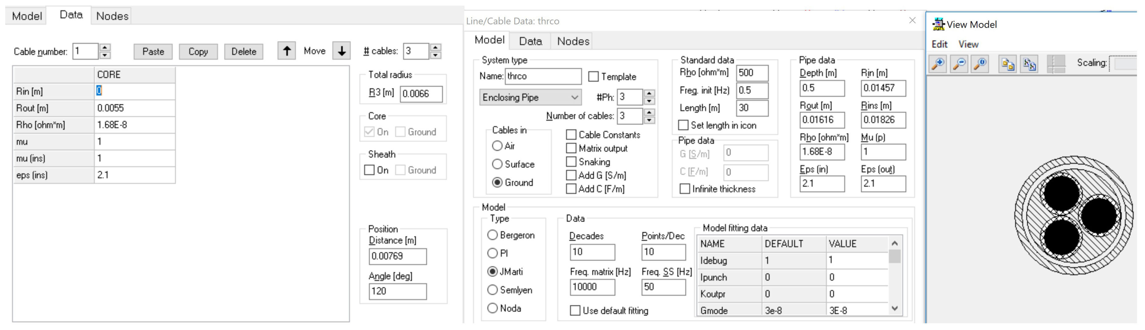
Appendix A. Details of the Cable and Line Models Used in the Simulations
Figure A1.
EMTP Line and Cables Constants data for the cable model.

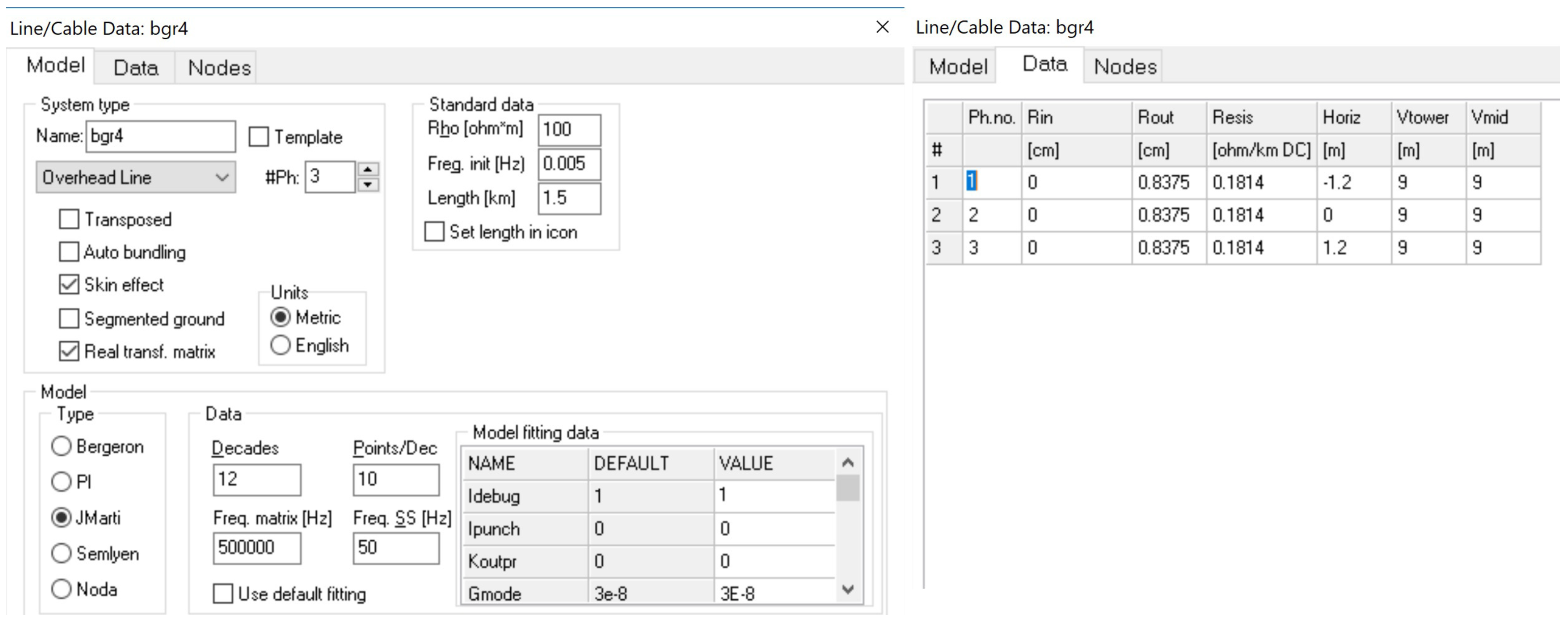
Figure A2.
EMTP Line and Cables Constants data for the line model.

Appendix B. EMTP VCO Model

References
- Ree, J.D.L.; Centeno, V.; Thorp, J.S.; Phadke, A.G. Synchronized Phasor Measurement Applications in Power Systems. IEEE Trans. Smart Grid 2010, 1, 20–27. [Google Scholar] [CrossRef]
- Tate, J.E.; Overbye, T.J. Line Outage Detection Using Phasor Angle Measurements. IEEE Trans. Power Syst. 2008, 23, 1644–1652. [Google Scholar] [CrossRef] [Green Version]
- Phadke, A.G. Synchronized phasor measurements in power systems. IEEE Comput. Appl. Power 1993, 6, 10–15. [Google Scholar] [CrossRef]
- Jenkins, N.; Long, C.; Wu, J. An Overview of the Smart Grid in Great Britain. Engineering 2015, 1, 413–421. [Google Scholar] [CrossRef] [Green Version]
- Low Voltage Current Sensor Technology Evaluation. Available online: https://www.westernpower.co.uk/projects/lv-sensors (accessed on 14 February 2019).
- Yang, B.; Katsaros, K.V.; Chai, W.K.; Pavlou, G. Cost-Efficient Low Latency Communication Infrastructure for Synchrophasor Applications in Smart Grids. IEEE Syst. J. 2018, 12, 948–958. [Google Scholar] [CrossRef] [Green Version]
- Aminifar, F.; Fotuhi-Firuzabad, M.; Safdarian, A.; Davoudi, A.; Shahidehpour, M. Synchrophasor Measurement Technology in Power Systems: Panorama and State-of-the-Art. IEEE Access 2014, 2, 1607–1628. [Google Scholar] [CrossRef]
- IEC/IEEE 60255-118-1:2018: IEEE/IEC International Standard—Measuring Relays and Protection Equipment—Part 118-1: Synchrophasor for Power Systems—Measurements. Available online: https://webstore.iec.ch/publication/28722 (accessed on 14 February 2019).
- Factors Affecting PMU Installation Costs, Technical Report. Available online: https://www.smartgrid.gov/files/PMU-cost-study-final-10162014_1.pdf. (accessed on 14 February 2019).
- Overholt, P.; Ortiz, D.; Silverstein, A. Synchrophasor Technology and the DOE: Exciting Opportunities Lie Ahead in Development and Deployment. IEEE Power Energy Mag. 2015, 13, 14–17. [Google Scholar] [CrossRef]
- Gharavi, H.; Hu, B. Scalable Synchrophasors Communication Network Design and Implementation for Real-Time Distributed Generation Grid. IEEE Trans. Smart Grid 2015, 6, 2539–2550. [Google Scholar] [CrossRef]
- Liu, Y.; Zhan, L.; Zhang, Y.; Markham, P.N.; Zhou, D.; Guo, J.; Lei, Y.; Kou, G.; Yao, W.; Chai, J.; et al. Wide-Area-Measurement System Development at the Distribution Level: An FNET/GridEye Example. IEEE Trans. Power Deliv. 2016, 31, 721–731. [Google Scholar] [CrossRef]
- DEDUCE: Determining Electricity Distribution Usage with Consumer Electronics. Available online: https://www.westernpower.co.uk/projects/deduce (accessed on 14 February 2019).
- Tan, G.; Robson, S.; Haddad, A. The Retrieval of Synchrophasors using Chirps. In Proceedings of the 2018 53rd International Universities Power Engineering Conference (UPEC), Glasgow, UK, 4–7 September 2018; pp. 1–6. [Google Scholar] [CrossRef]
- Distribution Network Visibility. Available online: http://innovation.ukpowernetworks.co.uk/innovation/en/Projects/tier-1-projects/distribution-network-visibility/ (accessed on 14 February 2019).
- Zhao, C.; Gu, C.; Li, F.; Dale, M. Understanding LV network voltage distribution- UK smart grid demonstration experience. In Proceedings of the 2015 IEEE Power Energy Society Innovative Smart Grid Technologies Conference (ISGT), Washington DC, USA, 18–20 February 2015; pp. 1–5. [Google Scholar] [CrossRef]
- Lu, S.; Repo, S.; Giustina, D.D.; Figuerola, F.A.; Löf, A.; Pikkarainen, M. Real-Time Low Voltage Network Monitoring—ICT Architecture and Field Test Experience. IEEE Trans. Smart Grid 2015, 6, 2002–2012. [Google Scholar] [CrossRef]
- IEEE Standard for Low-Frequency (Less Than 500 kHz) Narrowband Power Line Communications for Smart Grid Applications. Available online: https://0-ieeexplore-ieee-org.brum.beds.ac.uk/servlet/opac?punumber=6679208 (accessed on 14 February 2019).
- Berganza, I.; Sendin, A.; Arriola, J. PRIME: Powerline intelligent metering evolution. SmartGrids for Distribution, 2008. IET-CIRED. In Proceedings of the CIRED Seminar, Frankfurt, Germany, 23–24 June 2008; pp. 1–3. [Google Scholar]
- Robson, S.; Haddad, A.; Griffiths, H. Implementation of the Prime and G3-PLC Physical Layers in the EMTP-ATP. In Proceedings of the 2018 53rd International Universities Power Engineering Conference (UPEC), Glasgow, UK, 4–7 September 2018; pp. 1–6. [Google Scholar] [CrossRef]
- Robson, S.; Haddad, A.; Griffiths, H. A New Methodology for Network Scale Simulation of Emerging Power Line Communication Standards. IEEE Trans. Power Deliv. 2018, 33, 1025–1034. [Google Scholar] [CrossRef]
- Robson, A.; Haddad, S.; Griffiths, H. Simulation of Power Line Communication using ATP-EMTP and MATLAB. In Proceedings of the IEEE PES Conference on Innovative Smart Grid Technologies Europe, Gothenburg, Sweden, 11–13 October 2010; pp. 1–8. [Google Scholar] [CrossRef]
- Robson, S.; Griffiths, H.; Haddad, A. Narrowband Power Line Communications: Channel characteristics and modulation. In Proceedings of the 45th International Universities Power Engineering Conference UPEC 2010, Cardiff, UK, 31 August–3 September 2010; pp. 1–6. [Google Scholar]
- Artale, G.; Cataliotti, A.; Cosentino, V.; Cara, D.D.; Fiorelli, R.; Guaiana, S.; Tinè, G. A New Low Cost Coupling System for Power Line Communication on Medium Voltage Smart Grids. IEEE Trans. Smart Grid 2018, 9, 3321–3329. [Google Scholar] [CrossRef]
- Marti, J. Accurate Modelling of Frequency-Dependent Transmission Lines in Electromagnetic Transient Simulations. IEEE Trans. Power Apparatus Syst. 1982, PAS-101, 147–157. [Google Scholar] [CrossRef]
- Artale, G.; Cataliotti, A.; Cosentino, V.; Di Cara, D.; Fiorelli, R.; Russotto, P.; Tine, G. Medium Voltage Smart Grid: Experimental Analysis of Secondary Substation Narrow Band Power Line Communication. IEEE Trans. Instrum. Meas. 2013, 62, 2391–2398. [Google Scholar] [CrossRef]
- Xiaoxian, Y.; Tao, Z.; Baohui, Z.; Xu, N.H.; Guojun, W.; Jiandong, D. Investigation of Transmission Properties on 10-kV Medium Voltage Power Lines; Part I: General Properties. IEEE Trans. Power Deliv. 2007, 22, 1446–1454. [Google Scholar] [CrossRef]
- Harid, N.; Bogias, A.C.; Griffiths, H.; Robson, S.; Haddad, A. A Wireless System for Monitoring Leakage Current in Electrical Substation Equipment. IEEE Access 2016, 4, 2965–2975. [Google Scholar] [CrossRef] [Green Version]
- Robson, S.; Haddad, A.; Griffiths, H. Fault Location on Branched Networks Using a Multiended Approach. IEEE Trans. Power Deliv. 2014, 29, 1955–1963. [Google Scholar] [CrossRef]
- Robson, S.; Haddad, A.; Griffiths, H. Traveling Wave Fault Location Using Layer Peeling. Energies 2018, 12. [Google Scholar] [CrossRef]
Figure 1.
High Level block diagram of the proposed transmitter supporting two channels (voltage and current).
Figure 1.
High Level block diagram of the proposed transmitter supporting two channels (voltage and current).

Figure 2.
High level block diagram of the proposed receiver architecture, supporting n channels.

Figure 3.
Typical waveforms in the receiver.

Figure 4.
The simulation methodology is split into two domains. In the EMTP-ATP domain, two parallel simulations are performed; high frequency and power frequency. Post-simulation signals from both are saved in a PL4 file and automatically converted to a .MAT file for processing in the Matlab domain. The process is fully automated.

Figure 5.
Network under test. 12 transformers are modelled with secondary loads, . Transmitter points are labelled A-E.
Figure 5.
Network under test. 12 transformers are modelled with secondary loads, . Transmitter points are labelled A-E.

Figure 6.
Magnitude and Phase responses for the channel separating nodes in Feeder B, C, D and E with the observation point at the primary substation of Figure 5.
Figure 6.
Magnitude and Phase responses for the channel separating nodes in Feeder B, C, D and E with the observation point at the primary substation of Figure 5.

Figure 7.
Error variance as a function of used VCO bandwidth and SNR. Each point is obtained from 1000 Monte-Carlo simulations.
Figure 7.
Error variance as a function of used VCO bandwidth and SNR. Each point is obtained from 1000 Monte-Carlo simulations.

Figure 8.
Frequency spectra of the two Frequency Modulation (FM) channels at node B3.

Figure 9.
Error variance versus SNR for a used bandwidth of 78.5 Hz per transmitter channel. The Monte Carlo analysis (addition of noise) is performed after EMTP-ATP simulation. Each point is obtained from 1000 Monte-Carlo simulations.
Figure 9.
Error variance versus SNR for a used bandwidth of 78.5 Hz per transmitter channel. The Monte Carlo analysis (addition of noise) is performed after EMTP-ATP simulation. Each point is obtained from 1000 Monte-Carlo simulations.

Figure 10.
Magnitude and Phase responses for the channel separating nodes in Feeder B, C and D with the observation point at the primary substation of Figure 5.
Figure 10.
Magnitude and Phase responses for the channel separating nodes in Feeder B, C and D with the observation point at the primary substation of Figure 5.

Figure 11.
Box-whisker and distributions for power factor angle measurements resulting from 500 Monte Carlo simulations at a CNR of 30, 40 and 50 dB. The blue horizontal line represents the actual power factor angle.
Figure 11.
Box-whisker and distributions for power factor angle measurements resulting from 500 Monte Carlo simulations at a CNR of 30, 40 and 50 dB. The blue horizontal line represents the actual power factor angle.

Figure 12.
Box-whisker and distributions for harmonic measurements of the first 10 harmonics at a CNR of 40 dB and 30 dB for information sent from node B1.
Figure 12.
Box-whisker and distributions for harmonic measurements of the first 10 harmonics at a CNR of 40 dB and 30 dB for information sent from node B1.

Figure 13.
Difference between the actual and received phases at the voltage nodes at CNRs of 40 dB and 50 dB. The distributions are derived from 500 monte carlo simulations at each point.
Figure 13.
Difference between the actual and received phases at the voltage nodes at CNRs of 40 dB and 50 dB. The distributions are derived from 500 monte carlo simulations at each point.

Figure 14.
Photograph of built transmitter.

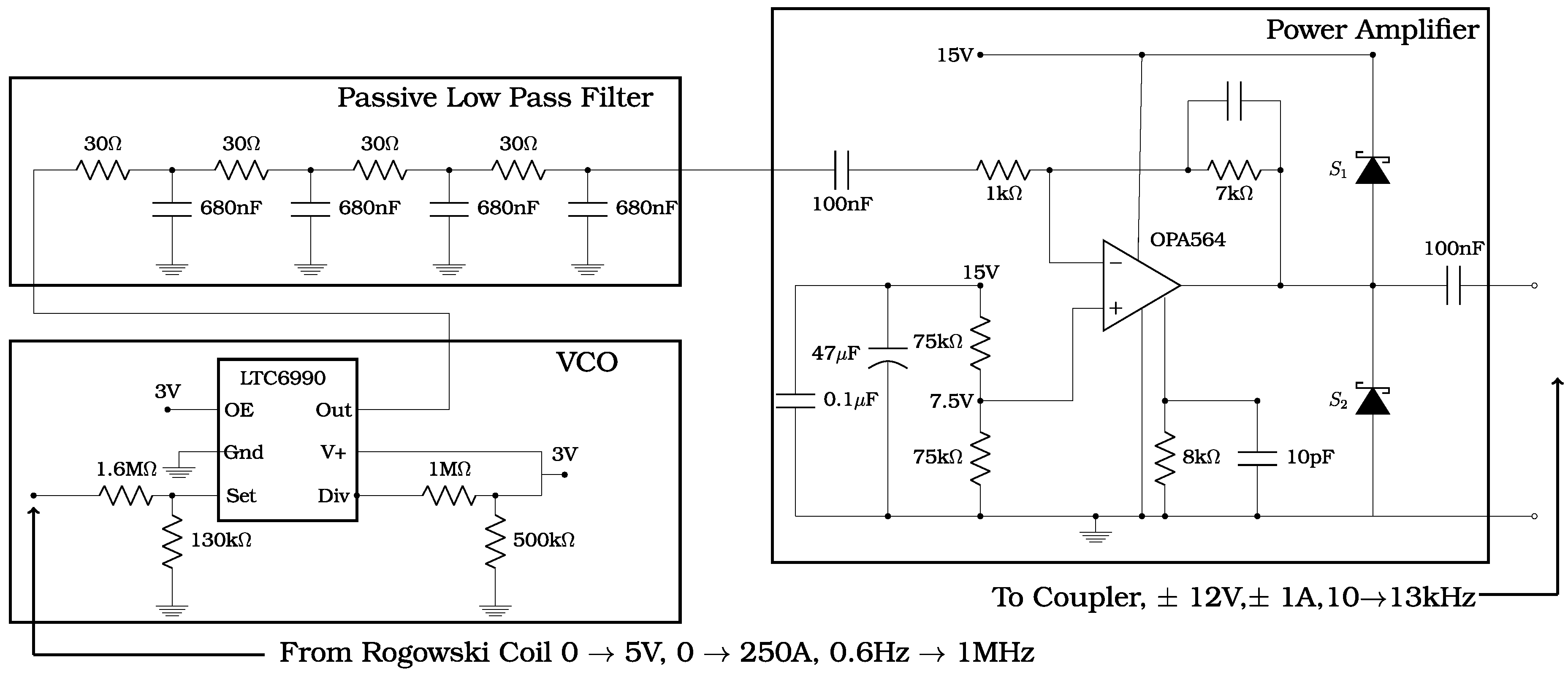
Figure 15.
Detailed Circuit Diagram of the transmitter design, showing the VCO, Passive Low Pass Filter and Power Operational Amplifier.
Figure 15.
Detailed Circuit Diagram of the transmitter design, showing the VCO, Passive Low Pass Filter and Power Operational Amplifier.

Figure 16.
Block diagram showing the FPGA hardware implementation of the Hilbert Transform. In the prototype, an N = 2048 point FFT and IFFT was used.
Figure 16.
Block diagram showing the FPGA hardware implementation of the Hilbert Transform. In the prototype, an N = 2048 point FFT and IFFT was used.

Figure 17.
High level Register Transfer Level (RTL) representation of the receiver design.

Figure 18.
RTL representation of the Hilbert Transform block.

Figure 19.
RTL representation of the “FFT for Power Analysis” block.

Figure 20.
Block diagram of the test setup.

Figure 21.
Photograph of the test setup.

Figure 22.
Plots showing the signals recorded by signaltap (real time debugging tool).

Figure 23.
Output of receiver as a function of measured current using a signal generator to produce the FM waveform.
Figure 23.
Output of receiver as a function of measured current using a signal generator to produce the FM waveform.

Figure 24.
Output of receiver as a function of measured current using the prototype transmitter.


Table 1.
Simulation Results for a CNR of 40 dB and a full range bandwidth of 78.5 Hz.
| Magnitude | FM Properties | Phase | |||||||
|---|---|---|---|---|---|---|---|---|---|
| Node | Received | Actual | Error (%) | ∠ Node | Received | Actual | Error (%) | ||
| VB1 | 984.12 V | 984.77 V | −0.07 | 15 kHz | 1.547 | ∠B1 | 3.55 | 2.81 | −20.7 |
| IB1 | 393.38 A | 392.47 A | 0.23 | 19 kHz | 0.616 | ||||
| VB2 | 984.12 V | 984.77 V | −0.07 | 23 kHz | 1.547 | ∠B2 | 2.52 | 3.64 | −30.77 |
| IB2 | 196.22 | 196.09 | 0.07 | 27 kHz | 0.308 | ||||
| VB3 | 982.59 V | 982.95 V | −0.15 | 31 kHz | 1.544 | ∠B3 | 1.68 | 1.82 | 8.33 |
| IB3 | 98.22 | 98.22 | 0.003 | 35 kHz | 0.154 | ||||
| VC1 | 966.49 V | 966.04 V | 0.05 | 39 kHz | 1.517 | ∠C1 | 18.54 | 17.44 | −5.93 |
| IC1 | 92.91 A | 92.16 A | 0.81 | 43 kHz | 0.145 | ||||
| VC2 | 966.71 V | 965.38 V | 0.14 | 47 kHz | 1.516 | ∠C2 | 6.19 | 6.04 | −2.42 |
| IC2 | 320.29 | 319.63 | 0.138 | 51 kHz | 0.502 | ||||
| VD1 | 938.56 V | 936.47 V | 0.22 | 55 kHz | 1.471 | ∠D1 | 17.26 | 17.44 | 1.04 |
| ID1 | 892.54 | 893.40 | −0.098 | 59 kHz | 1.403 | ||||
| VD2 | 939.91 V | 939.77 V | 0.015 | 63 kHz | 1.471 | ∠D2 | 17.61 | 17.44 | −0.96 |
| ID2 | 897.19 | 896.55 | 0.07 | 67 kHz | 1.408 | ||||
| VE1 | 929.81 V | 930.38 V | −0.06 | 71 kHz | 1.461 | ∠E1 | 26.35 | 17.61 | 33.18 |
| IE1 | 879.31 | 882.60 | −0.37 | 75 kHz | 1.386 | ||||
| VE2 | 939.91 V | 939.77 V | −0.06 | 79 kHz | 1.476 | ∠E2 | 17.65 | 17.68 | 0.17 |
| IE2 | 1769.22 | 1768.32 | 0.05 | 83 kHz | 2.778 | ||||
Table 2.
Summary of resource usage for the receiver design.
| Board | Cyclone V GX Starter Kit |
| FPGA Family | Cyclone V |
| Device | 5CGXFC5C6F27C7 |
| Logic Utilization (in ALMs) | 20,669/29,080 (71%) |
| Total Registers | 35,899 |
| Total Pins | 12/364 (3%) |
| Total block memory bits | 2,333,840/4,567,040 (51%) |
| Total DSP Blocks | 92/150 ( 61% ) |
| PLLs | 1/12 (8%) |
| Power Analysis Block Usage | 4782 ALMs |
| Hilbert Transform Block Usage | 12,747 ALMs |
© 2019 by the authors. Licensee MDPI, Basel, Switzerland. This article is an open access article distributed under the terms and conditions of the Creative Commons Attribution (CC BY) license (http://creativecommons.org/licenses/by/4.0/).
Share and Cite
MDPI and ACS Style
Robson, S.; Tan, G.; Haddad, A. Low-Cost Monitoring of Synchrophasors Using Frequency Modulation. Energies 2019, 12, 611. https://0-doi-org.brum.beds.ac.uk/10.3390/en12040611
AMA Style
Robson S, Tan G, Haddad A. Low-Cost Monitoring of Synchrophasors Using Frequency Modulation. Energies. 2019; 12(4):611. https://0-doi-org.brum.beds.ac.uk/10.3390/en12040611
Chicago/Turabian StyleRobson, Stephen, Gan Tan, and Abderrahmane Haddad. 2019. "Low-Cost Monitoring of Synchrophasors Using Frequency Modulation" Energies 12, no. 4: 611. https://0-doi-org.brum.beds.ac.uk/10.3390/en12040611
Note that from the first issue of 2016, this journal uses article numbers instead of page numbers. See further details here.