Power Flow Analysis of the Advanced Co-Phase Traction Power Supply System

Abstract

The development of the traction power supply system (TPSS) is limited by the existence of the neutral section in the present system. The advanced co-phase traction power supply system (ACTPSS) can reduce the neutral section completely and becomes an important research and development direction of the railway. To ensure the stable operation of ACTPSS, it is necessary to carry out an appropriate power analysis. In this paper, the topology of advanced co-phase traction substation is mainly composed by the three-phase to single-phase cascaded converter. Then, the improved PQ decomposition algorithm is proposed to analyze the power flow. The impedance model of the traction network is calculated and established. The power flow analysis and calculation of the ACTPSS with different locations of locomotive are carried out, which theoretically illustrates that the system can maintain stable operation under various working conditions. The feasibility and operation stability of the ACTPSS are verified by the simulations and low power experiments.

1. Introduction

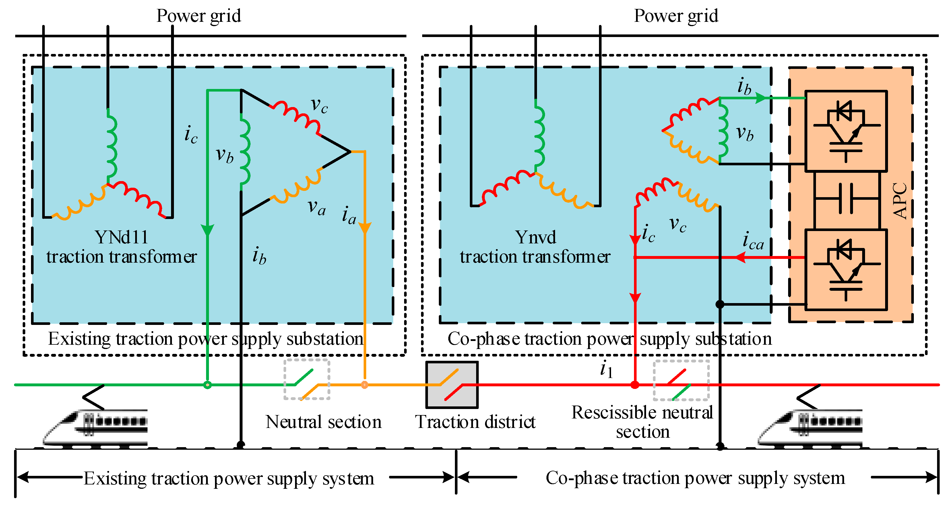
By the end of 2018, the operation mileage of the China railway had already reached 124 thousands kilometers. Among them is the high speed railway mileage, which reached 22 thousands kilometers. There is no doubt that the China railway is of great importance to China’s transportation industry. To the railway system, the traction power supply system (TPSS) is a crucial part that maintains stable and safe operation of railways [1,2,3]. The existing TPSS is shown in the left of Figure 1. The power supply distance of each traction substation is limited by the neutral sections, and the power supplied by each traction substation is incapable of interconnection [4,5,6,7]. As a result, when the train is running in regenerative braking mode, the power cannot be used by other locomotives because of the neutral sections. Then, the power is transmitted to a three-phase grid through the transformer, which causes the problem of large harmonic content and unbalanced voltage in three-phase power network. Because of the regenerative braking energy consumption, a large number of economic losses are caused [4]. Furthermore, the voltage range of the traction network is changed sharply, and the negative sequence, reactive power, and harmonic problems are brought into the present TPSS when the locomotives are under operation [8,9]. These problems influence the quality of the three-phase power grid, the operation efficiency, and the stability of the TPSS. Moreover, the locomotives need to decelerate and slide through the neutral section. In this way, the loss of speed and the decrease of the operation safety are problems that restrict the development of railways [10,11].

To solve these problems, a great deal of research has been done in China. The co-phase traction power supply system (CTPSS) is proposed in [10], which is shown in the right of Figure 1. The active power compensators (APC) is applied in the CTPSS [4]. Half of the neutral sections can be reduced, and the power quality of the three-phase power grid can be improved to a certain extent [6]. The CTPSS has been put into operation in Meishan, Sichuan province. Voltage source converter based high voltage direct current transmission traction power supply system (VSC-Based HVDC TPSS) is proposed in [5]. Compared to TPSS, the power quality problems such as unbalance, reactive power, and harmonic distortion are greatly improved. However, the stray current is generated by the HVDC TPSS, which is harmful to the rail system, and the current supply voltage of the traction network (27.5 kV/50 Hz) is not changed by CTPSS. If there is a line using DC system, the trains will not be able to run on both systems at the same time.

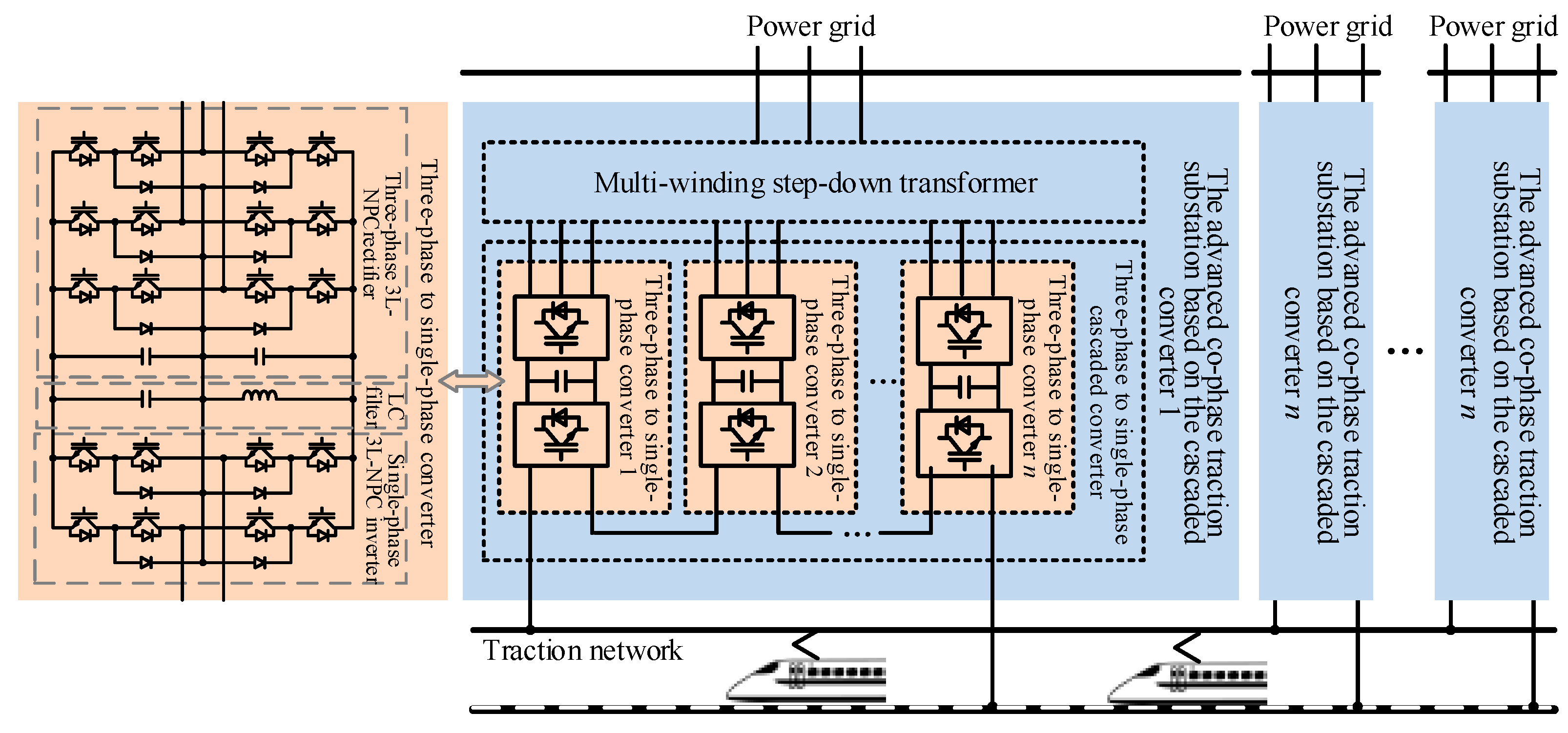
In order to link all the traction networks of every different substation, the advanced traction power substation system is proposed in literature [12]. The substation based on three-phase to single-phase converter is adopted in this system [13,14,15,16]. In order to adapt to the voltage level of three-phase grid voltage and the traction network voltage, the step-down transformer and step-up transformer are added to the three-phase grid and the traction network side, respectively. The neutral sections and problems of power quality in the traditional system can be avoided. However, it is difficult to meet the existing substation requirement of capacity because the structure is limited by the power electronic devices. The advanced co-phase traction power supply system (ACTPSS) based on three-phase to single-phase cascaded converter is proposed in literature [7], as shown in Figure 2. The ACTPSS achieves the interconnection of the whole traction network, thus all the neutral sections are reduced by ACTPSS. The negative sequence, reactive power, and harmonic problems existent in the traditional TPSS can be solved effectively [12,13]. Meanwhile, the voltage of the traction network can be maintained in a relatively stable range, and regenerative braking energy can be better utilized. Thus, the ACTPSS has become essential in the research and development of future TPSS.

Due to the interconnection of the whole traction network, the energy of the locomotive is mainly supplied by the closest power supply arm, and the adjacent substations provide the remaining parts of the energy. Therefore, the system capacity of the traction power supply system can be reduced. To assess and manage the operation state of ACTPSS, the power flow analysis also needs to be researched. Criteria of voltage stability based on the existence of the power flow solvability was used in the power distribution network [17]. Another voltage stability criterion was obtained based on the volt-ampere characteristic of the branches in the system [18]. This power analysis research of the public three-phase power grid provides a good theoretical basis for the power flow analysis of the traction network. In the power supply model of auto transformer (AT) traction substation, the power flow and voltage distribution in different working conditions of high-speed railway are analyzed by establishing a general multi-conductor chain circuit model [19,20]. The influence of traction load on power quality of the three-phase power grid was illustrated. These laid a good foundation for building the model of the traction network [21,22]. In ACTPSS, no node voltage of the traction network is allowed to exceed the prescribed voltage standard [23]. In this way, each traction substation supplies the power equitably and stably. Furthermore, the voltage range of the traction network maintains steadily. Therefore, it is necessary to carry out the power flow analysis of ACTPSS and assess the voltage variation degree of the traction network so that the dispatchers can take correspondent measures.

In this paper, firstly, the structure of ACTPSS based on a three-phase to single-phase cascaded converter is illustrated, and the corresponding control strategy and modulation strategy are given. Secondly, on the basis of ACTPSS, the mathematical model of traction network impedance is established by multi-conductor model, and the power flow analysis of the traction network is carried out by the improved PQ decomposition algorithm. Thirdly, the stability performance of ACTPSS is verified through the analysis of the power flow under different locomotive operation conditions. Finally, the correctness of the theory analysis is verified through the simulation, and the operation reliability of ACTPSS is verified through the low power experiment.

2. Configurations and Strategy

2.1. The Structure of ACTPSS

According to the structure of ACTPSS, as shown in Figure 2, the traction substation consists of the multi-winding step-down transformer and the three-phase to single-phase cascaded converter. The primary side of the multi-winding step-down transformer is connected with the three-phase power grid, and the secondary sides of it are connected with the three-phase to single-phase converters. To improve the withstand voltage of the traction substation, the cascaded topology is utilized in each traction substation. In order to improve the withstand voltage of the single model, the three-level neutral point clamped (3L-NPC) topology is adopted in this paper.

The three-phase to single-phase converter is comprised of the three-phase 3L-NPC rectifier and the single-phase 3L-NPC inverter. The three-phase 3L-NPC rectifier converts the power from three-phase alternating current (AC) to direct current (DC), then the single-phase 3L-NPC inverter converts the power from DC to single-phase AC. The output of the three-phase to single-phase cascaded converter as the output of the traction substation is connected with the traction network. The amplitude, the frequency, and the phase of the traction substation output voltage are controlled to be in accordance with the traction network. The traction substations are paralleled with the traction network and achieve the power interconnection of the whole system.

2.2. The Control Strategy and Modulation Strategy of Three-Phase 3L-NPC Rectifier

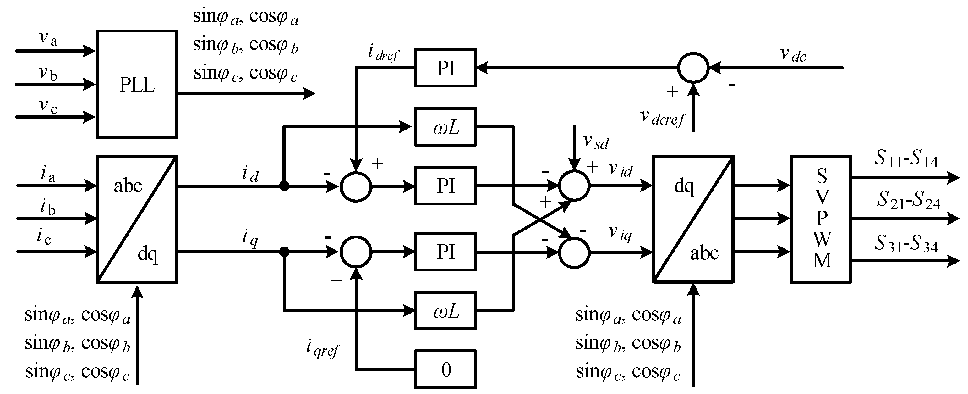
In order to ensure that the three-phase 3L-NPC rectifiers operate under unit power factor, P-Q transformation, voltage, and current double closed loop control strategy is adopted [24]. The control strategy and modulation strategy of the three-phase 3L-NPC rectifier are illustrated by Figure 3. Firstly, the phase of input voltage v_abc is extracted through phase lock loop (PLL). The locked phase is used as the reference phase of input current i_abc to achieve coordinate transformation from the three-phase static coordinate (abc) to the two-phase rotating coordinate (dq). Under the two-phase rotating coordinate, the active component and reactive component of the current are controlled, respectively. The reference of the active component of the current is relative with the output voltage v_dc, while the reference of the reactive component of the current is 0. The Space Vector Pulse Width Modulation (SVPWM) strategy is adopted as the modulation strategy for the rectifier.

2.3. The Control Strategy and Modulation Strategy of Single-Phase 3L-NPC Cascaded Inverter

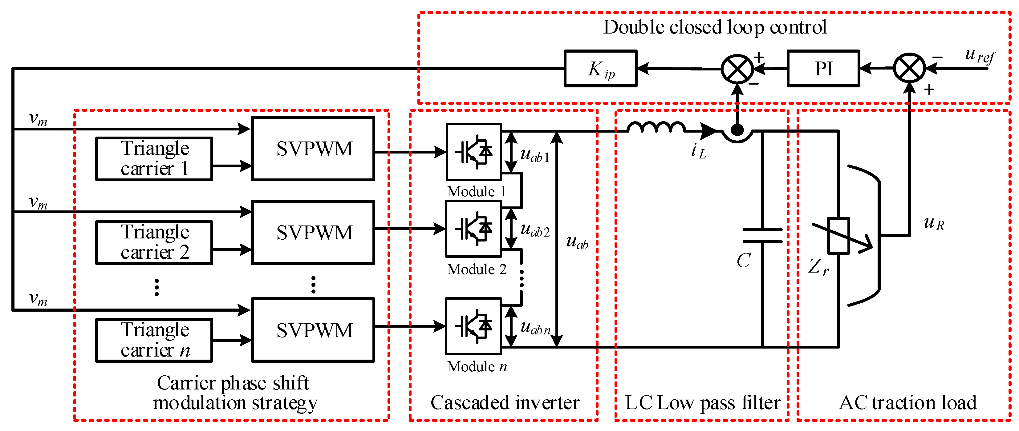
The control strategy and modulation strategy of the single-phase 3L-NPC cascaded inverter are shown in Figure 4. The double closed loop control strategy is applied in this paper. The outer loop control strategy is designed to steady the output voltage. The inner loop control strategy is designed to adjust the dynamic response of the system. The value of output voltage and inductance current are detected to involve the control strategy.

The carrier phase shift strategy is used as the modulation strategy [25]. Every inverter model has the same modulation wave produced by the controller, while the triangle angle waves are different. The phase angle difference of two adjacent triangle angle waves is π/n, where the n represents the number of the inverter models. The single-phase SVPWM strategy is used as the modulation strategy to drive each inverter model.

3. The Traction Network Impedance Model of ACTPSS

Because the steel rail and ground belong to ferromagnetic materials, the current of the circuit changes with the operation state change of the traction load, which has great influence on the equivalent inductance and impedance of the steel rail. Generally, the length of steel rail is recognized as infinity, and the distribution parameters between the steel rail and ground are nonlinear. Furthermore, the traction impedance is also recognized as nonlinear. Compared with the impedance calculation of the power system, the impedance calculation of the traction network is much more complicated. In this paper, the impedance model of the traction network based on ACTPSS is built by the method of the simplified equivalent model.

3.1. The Simplified Equivalent Model of Traction Network

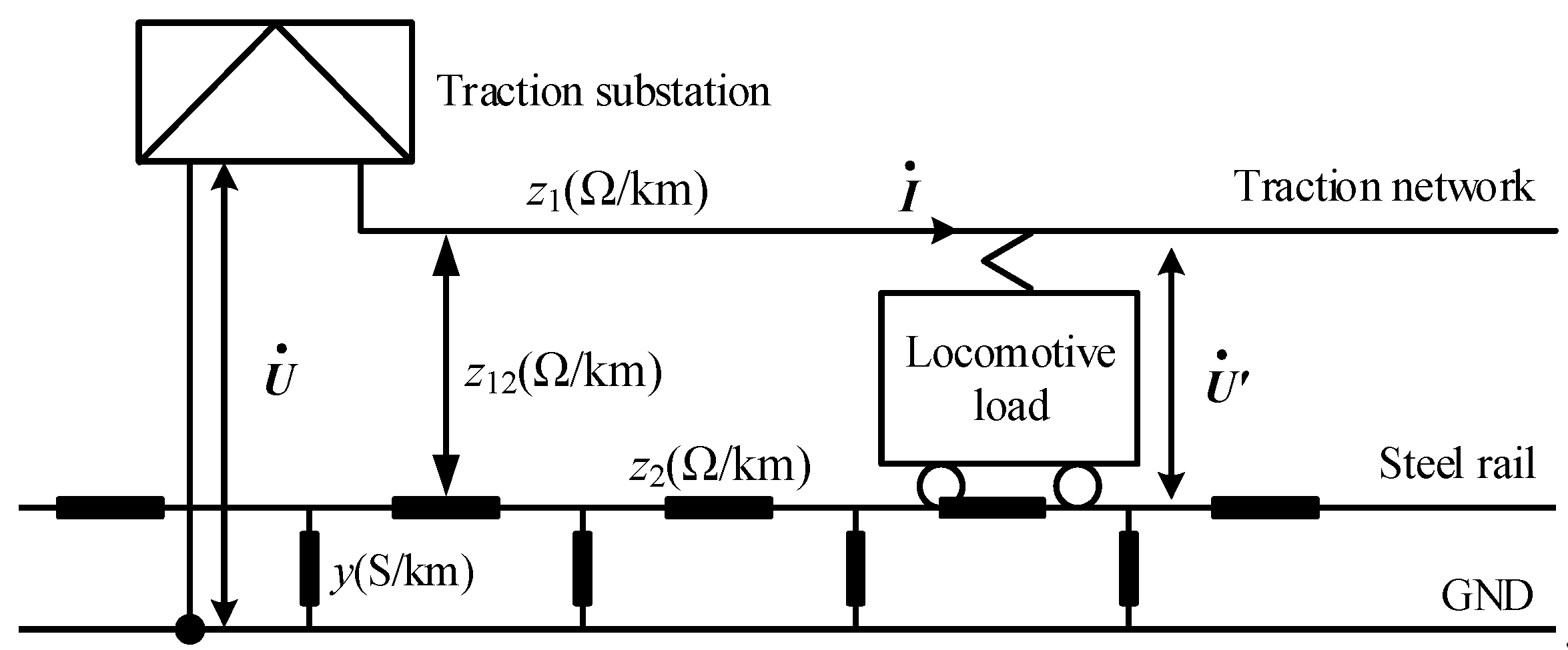
The original circuit model of the traction network is shown in Figure 5. Viewed from the output port of the traction substation, the impedance of the traction network consists of several equivalent impedances of the conductor-ground circuit [26].

According to Figure 5, it is known that the unit length impedance of traction network z can be calculated by Equation (1):

$$z=\frac{\stackrel{·}{U}-\stackrel{·}{U^{\prime }}}{\stackrel{·}{I}l}$$

(1)

In Equation (1), the voltage between the output port of the traction substation and ground is $\stackrel{·}{U}$, the voltage of the locomotive load is $\stackrel{·}{U^{\prime }}$, the length of the traction network is l, and the current of the traction network is $\stackrel{·}{I}$.

It is known from Equation (1) that the z is nonlinear and cannot be calculated by formula flexibly. It is assumed that the current of steel rail can flow into the ground instantly, or the current of the ground can flow into the steel rail instantly, and the current can flow into the output port of the traction substation with the same amplitude as well. Then, the admittance γ between the steel rail and the ground can be considered to approach infinity, and the conduction current of steel rail can be considered to tend to 0. Taking these assumptions as the simplification condition, Equation (2) can be expressed as:

$$\underset{\gamma \to \infty }{\lim }\frac{1}{2}(1-k_z)\stackrel{·}{I}\left[e^{-\gamma \left(l-x\right)}+e^{-\gamma x}\right]\approx 0$$

(2)

In Equation (2), $k_z=z_{12}/z_2$. The mutual impedance is z₁₂, the self-impedances are z₁ and z₂, and the distance between the locomotive and the traction substation is x.

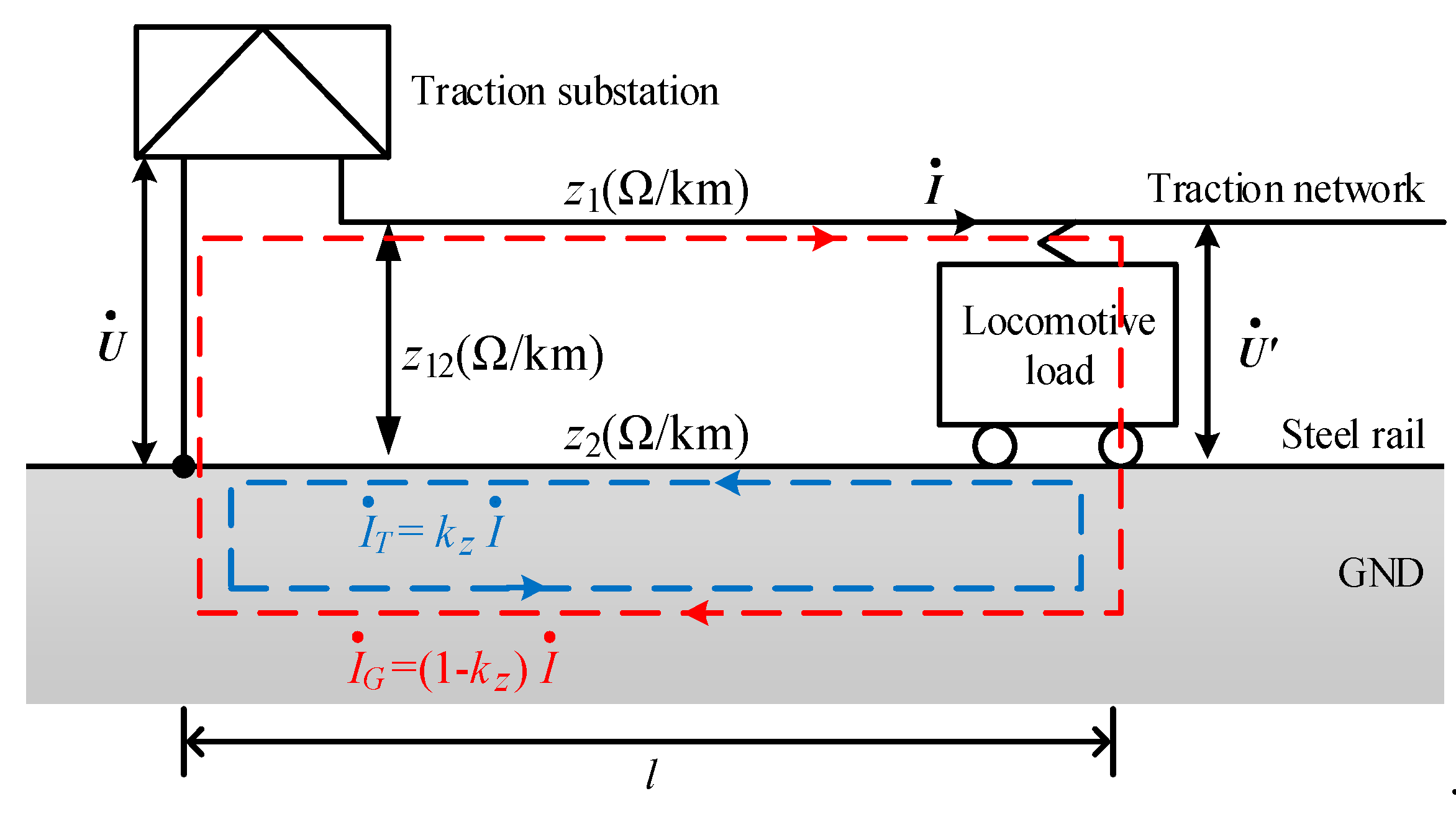
Then, the current of the steel rail $\stackrel{·}{I_T}$ and the ground $\stackrel{·}{I_G}$ can be recognized as:

$$\{\begin{array}{l}\stackrel{·}{I_T}\left(x\right)=\stackrel{·}{I_T}=k_z\stackrel{·}{I}\\ \stackrel{·}{I_G}\left(x\right)=\stackrel{·}{I_G}=\left(1-k_z\right)\stackrel{·}{I}\end{array}$$

(3)

The simplified impedance model of the traction network is illustrated by Figure 6 [26]. The model is composed of two current loops. In the first loop, the current flows through the traction network and the ground. In the second loop, the current flows through the steel rail and the ground. The second current loop just reflects the induced current, which is far bigger than the conduction current. According to the light of this simplified impedance model, the unit length impedance of the traction network z can be figured out by the calculation of the self-impedance of the first and second loop.

According to the Carson theory [27], the ground can be recognized as virtual wire. Then, Equation (4) can be expressed as:

$$\{\begin{array}{ll}{z}_1=r_1+0.05+j0.1446g\frac{D_g}{R_{\epsilon 1}}& \mathsf{\Omega }/\mathrm{km}\\ z_2=r_2+0.05+j0.1446g\frac{D_g}{R_{\epsilon 2}}& \mathsf{\Omega }/\mathrm{km}\\ z_{12}=0.05+j0.1446g\frac{D_g}{d_{12}}& \mathsf{\Omega }/\mathrm{km}\end{array}$$

(4)

In Equation (4), the r₁ and R_g1 represent the effective resistance and equivalent radius of the first loop, respectively; r₂ and R_g2 represent the effective resistance and equivalent radius of the second loop, respectively; the D_g represents the depth of the equivalent earth-return circuit; d₁₂ is the center distance between the conductor in the first and second loop.

Therefore, the z can be calculated as follow:

$$z=z_1-\frac{z_{12}{}^2}{z_2}$$

(5)

According to Equation (5), the impedance of the traction network z_l with the length l can be expressed as follows:

$$z_l=z\times l$$

(6)

3.2. The Impedance Calculation for the Traction Network of ACTPSS

In ACTPSS, the induced current is far bigger than the conduction current of the second loop. When the distance between locomotive and traction substation is longer than 5 km, the conduction current can be ignored, and the impedance of the traction network can only be calculated by the inducted current. Generally, the error between the calculation result and the actual model is within 5%. Therefore, the simplified equivalent model of the traction network is always adopted. The wire type of GLCA-100/215 was selected as the traction network wire in this paper. Then, r₁ = 0.184 Ω/km, r₂ = 0.295 Ω/km, R_g1 = 8.56 mm, R_g2 = 12.2 mm, d₁₂ = 5850 mm. According to the simplified equivalent model of the traction network, the impedance can be calculated as shown in

Table 1. The impedance calculation results of the traction network.

The Type of Impedance	Value
The self-impedance of traction network	z1 = 0.234 + j0.728 (Ω/km)
The self-impedance of steel rail	z2 = 0.345 + j0.706 (Ω/km)
The mutual impedance	z12 = 0.05 + j0.318 (Ω/km)
The unit length impedance of traction network	z = 0.2527 + j0.598 (Ω/km)

.

4. The Power Flow Analysis for Traction Network of ACTPSS

4.1. The Improved PQ Decomposition Algorithm

The PQ decomposition algorithm, which can be used to calculate the power flow, is based on the simplified power flow calculation progress of the polar coordinate formula in the Newton-Raphson algorithm [28]. Generally, in the transmission line equivalent model of the AC high voltage power grid, it is considered that x >> r, where the x is the line reactance and r is the line impedance. Therefore, the active power is mainly affected by the voltage phase, while the reactive power is mainly affected by the voltage amplitude. If the effect of voltage phase change on reactive power distribution and the effect of voltage amplitude change on active power distribution are ignored, Equations (7) and (8) can be obtained as follows:

$$\Delta P=H\Delta \theta$$

(7)

$$\Delta Q=L{U}^{-1}\Delta U$$

(8)

From Equations (7) and (8), it is known that the correction equation of the active power ΔP and the reactive power ΔQ can be iterated, respectively. Compared with the 2n-order linear equations of the Newton-Raphson algorithm, the PQ decomposition algorithm transforms it into two n-order linear equations. The calculation time can be reduced sharply. However, in the iteration, the coefficient matrix H and L, which belong to the asymmetric matrix, are changing constantly. Thus, it is necessary to change coefficient matrices into the symmetric matrices so that the calculation can be further simplified. Because of the relatively little voltage phase difference between two ports of the circuit, it can be supposed as follows:

$$\{\begin{array}{l}\cos {\delta }_{ij}\approx 1\\ G_{ij}\sin {\delta }_{ij}\ll B_{ij}\\ \begin{array}{c}{Q}_i\ll U_i^2{B}_{ii}\end{array}\end{array}$$

(9)

Then, the expression of the Jacobian matrix can be expressed as:

$$H_{ij}=L_{ij}=U_i{U}_j{B}_{ij}$$

(10)

$$H_{ii}=L_{ii}=U_i^2{B}_{ii}$$

(11)

Then, Equations (7) and (8) can be rewritten as:

$$\Delta P=UBU\Delta \theta$$

(12)

$$\Delta Q=UBU\left(U^{-1}\Delta U\right)=UB\Delta U$$

(13)

In Equations (12) and (13), the U is the diagonal matrix of the effective value of node voltage, and the B represents the susceptance matrix.

By multiplying Equations (12) and (13) with U⁻¹, Equations (14) and (15) can be obtained as follows:

$$U^{-1}\Delta P=B^{\prime }U\Delta \theta$$

(14)

$$U^{-1}\Delta Q=B^{″}\Delta U$$

(15)

The matrix forms are shown as follows:

$$\left[\begin{array}{c}\Delta P_1/U_1\\ \Delta P_2/U_2\\ ⋮\\ \Delta P_n/U_n\end{array}\right]=B^{\prime }\left[\begin{array}{c}{V}_1\Delta {\theta }_1\\ V_2\Delta {\theta }_2\\ ⋮\\ V_n\Delta {\theta }_n\end{array}\right]$$

(16)

$$\left[\begin{array}{c}\Delta Q_1/U_1\\ \Delta Q_2/U_2\\ ⋮\\ \Delta Q_m/U_m\end{array}\right]=-B^{″}\left[\begin{array}{c}\Delta U_1\\ \Delta U_2\\ ⋮\\ \Delta U_m\end{array}\right]$$

(17)

In Equations (16) and (17), the coefficient matrices B′ and B″ have the same form. The B′ is the n order matrix and the B″ is the n – m − 1 order matrix, where the m represents the number of the PV node. Both the B′ and B″ are imaginary parts of the admittance matrix, and both are symmetric matrices.

However, the transmission line reactance of the traction network in ACTPSS is not much larger than the resistance, thus the PQ decomposition algorithm cannot be applied directly. Based on the PQ decomposition algorithm, the improved PQ decomposition algorithm is proposed to calculate the power flow of the traction network.

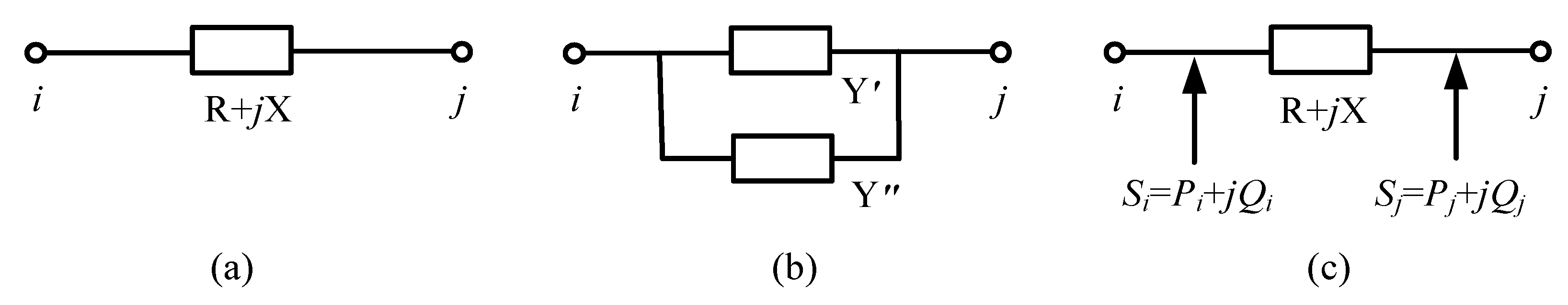
The impedance model of the traction network is shown in Figure 7a. The model after simplifying the impedance between node i and node j into the two parallel impedances model is shown in Figure 7b. The value of the simplified model is identical to the original mode. The value of the simplified model can be expressed as Equation (18):

$$\{\begin{array}{l}{Y}^{\prime }=-j\frac{1}{X}\\ Y^{″}=\frac{R}{R^2+X^2}+j\left(\frac{1}{X}-\frac{X}{R^2+X^2}\right)\end{array}$$

(18)

In Equation (18), the X is the line reactance of the original model, the R is the line resistance of the original model, and the unit of them is Ω. If we suppose that the real part of the Y″ is 0, the transmission line reactance of the traction network can be sufficiently larger than the resistance, and the condition G_ijsinδ_ij << B_ij can be satisfied. To make sure that the power flow calculation will not be wrong and the system can keep balance after the change of the impedance, the lacking power part will be added by the other power sources in node i and node j. The way to add the power sources can be determined by Figure 7c. Combined with the node voltage and the modified Y″, the power of node i and node j can be illustrated as:

$$\{\begin{array}{l}{P}_i=U_i\left[G^{″}\left(U_j\cos {\theta }_{ij}-U_i\right)+B^{″}{U}_j\sin {\theta }_{ij}\right]\\ Q_i=U_i\left[G^{″}{U}_j\sin {\theta }_{ij}+B^{″}\left(U_j\cos {\theta }_{ij}-U_i\right)\right]\\ P_j=U_j\left[G^{″}\left(U_i\cos {\theta }_{ij}-U_j\right)+B^{″}{U}_i\sin {\theta }_{ij}\right]\\ Q_j=-U_j\left[G^{″}{U}_i\sin {\theta }_{ij}+B^{″}\left(U_i\cos {\theta }_{ij}-U_j\right)\right]\end{array}$$

(19)

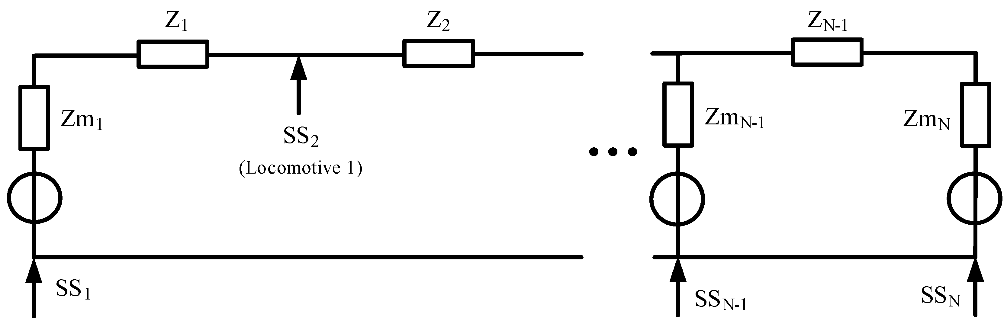
In Equation (19), the G’’ is the conductance of the modified model, the B’’ is the susceptance of the modified model, and the unit of them is S. When the condition G_ijsinδ_ij << B_ij has been satisfied, the subsequent calculation of the improved PQ decomposition algorithm is same as the PQ decomposition algorithm. In the power flow calculation of the improved PQ decomposition algorithm to the traction network, the locomotives are considered as the power sources, and the traction substations are recognized as the equivalent node models of voltage source. The equivalent mathematic model of ACTPSS, which can apply the improved PQ decomposition algorithm, is exhibited in Figure 8.

4.2. The Power Flow Calculation of ACTPSS

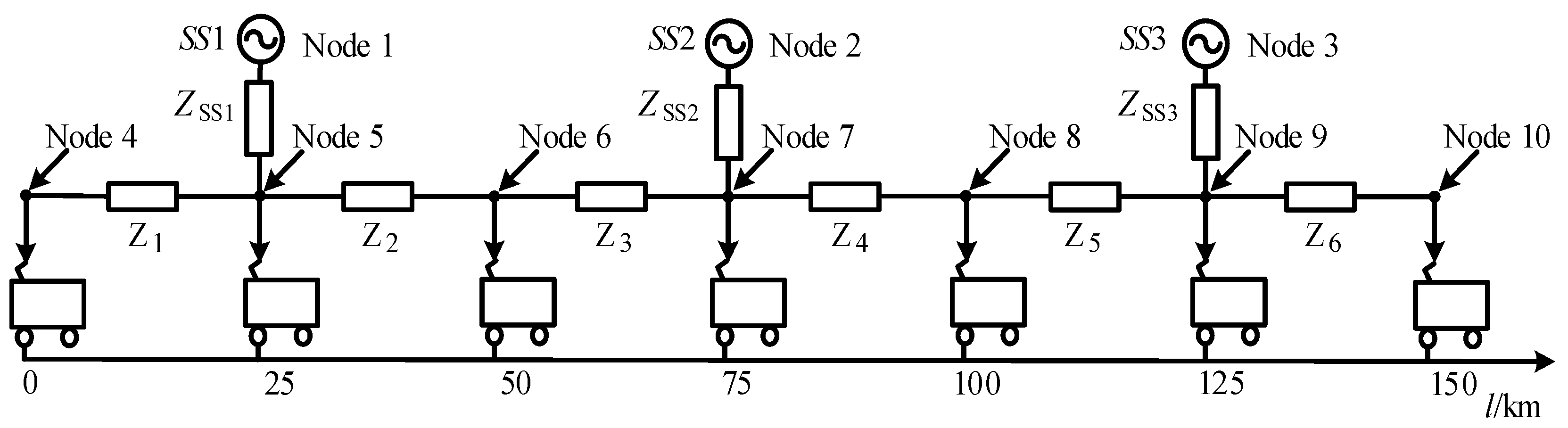
In this section, the improved PQ decomposition algorithm is applied to calculate the power flow and to verify the operation stability of the system. The software PAST is used to build the model shown by Figure 9. The model consists of three traction substations and seven locomotives and simulates the condition in which several locomotives run in a certain section. The type of locomotive is CRH380A, the active power is 9600 kW, and the power factor is 0.99.

Under the ideal state, the output voltages of traction substation SS1, SS2, and SS3 are coincidental, thus they can be recognized as the balanced node. The Z_SS1, Z_SS2, and Z_SS3 represent the resistances of the three traction substations, respectively. The value of them is set as 0.5 + j3.375 Ω in this model. The Z_i (i = 1, 2 …6) represents the resistance of the traction network, and the value of unit length is set as 0.2527 + j0.298 Ω. The L_i (i = 1, 2, …7) represents the seven locomotives, respectively, and the locomotive can be seen as a PQ node because the power of locomotive is constant. In conclusion, the system model is composed of 10 nodes.

Power flow calculation results of ACTPSS are listed in

Table 2. The power flow calculation results of ACTPSS.

Node	Voltage Amplitude U (kV)	Voltage Phase α (rad)	Complex Power S (MVA)
1	27.500	0.000	25.484 + j10.218
2	27.500	0.000	21.159 + j6.625
3	27.500	0.000	25.484 + j10.218
4	21.3758	−0.35922	−9.6 + j(−1.37)
5	25.9499	−0.11363	−9.6 + j(−1.37)
6	24.3719	−0.20953	−9.6 + j(−1.37)
7	26.4185	−0.09387	−9.6 + j(−1.37)
8	24.3719	−0.20953	−9.6 + j(−1.37)
9	25.9499	−0.11363	−9.6 + j(−1.37)
10	21.3758	−0.35922	−9.6 + j(−1.37)

. In this paper, the voltage values of node 4 and node 10 in the model are the lowest, which are 21.3758 kV. Obviously, 21.3758 kV is still higher than 19 kV. At this condition, the locomotive can continue to run, which indicates that ACTPSS proposed in this paper can ensure the locomotive operates normally.

The line impedance exists in the traction network model. By using the node voltage and node admittance matrix, it can be calculated that the total power of the system is 72.135 + j27.062 MVA, the total consumption power of the system load is 67.2 + j9.595 MVA, and the total power loss of the system is 4.935 + j17.472 MVA. The power loss of every line between two nodes is illustrated in

Table 3. The power losses of ACTPSS.

Line	Power Losses	Line	Power Losses
1–5 line	0.499 + j3.365	6–7 line	0.307 + j0.726
2–7 line	0.325 + j2.194	7–8 line	0.307 + j0.726
3–9 line	0.499 + j3.365	8–9 line	0.199 + j0.471
4–5 line	1.3 + j3.077	9–10 line	1.3 + j3.077
5–6 line	0.199 + j0.471	Total	4.935 + j17.472

. The power losses are expressed in the form of complex power with the inductive reactive power. Because the distance between the locomotive and the node is different, the power loss of the line between the nodes is different.

4.3. The Calculation of Output Power Under Different Locomotive Location

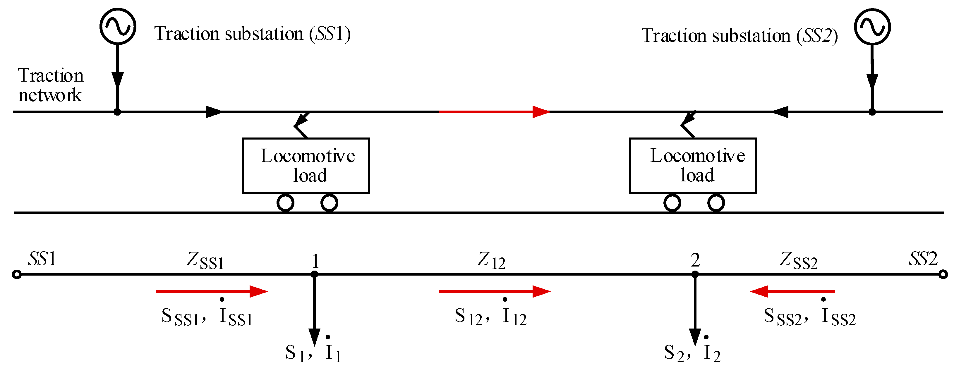
Since the different location of the locomotive directly affects the output power of each traction substation, the influence of different locomotive locations on the output power of substation with two traction substations is analyzed as an example. The model is established in Figure 10.

Two locomotives are located at point 1 and 2 in Figure 10. The locomotive is considered as a single-particle model in the analysis. The output current of traction substations SS1 and SS2 are i_SS1 and i_SS2, respectively. The line impedances between the traction substations SS1 and SS2 to the locomotive are Z_SS1 and Z_SS2, respectively. The line impedance between point 1 and point 2 is Z₁₂. The currents of locomotives 1 and 2 are i₁ and i₂, respectively.

According to the Kirchhoff’s Voltage Law (KVL) and Kirchhoff’s Current Law (KCL):

$${\stackrel{·}{V}}_{SS1}-{\stackrel{·}{V}}_{SS2}=Z_{SS1}{\stackrel{·}{I}}_{SS1}+Z_{12}{\stackrel{·}{I}}_{12}-Z_{SS2}{\stackrel{·}{I}}_{SS2}$$

(20)

$${\stackrel{·}{I}}_{SS1}-{\stackrel{·}{I}}_{12}=\stackrel{·}{I_1}$$

(21)

$${\stackrel{·}{I}}_{12}-{\stackrel{·}{I}}_{SS2}={\stackrel{·}{I}}_2$$

(22)

Assuming that the output voltage of the SS1 and SS2 are V_SS1 and V_SS2, and the currents I₁, I₂ of the locomotive are known, then Equations (21) and (22) can be simplified as:

$${\stackrel{·}{I}}_{SS1}=\frac{\left(Z_{12}+Z_{SS2}\right)\stackrel{·}{I_1}+Z_{SS2}{\stackrel{·}{I}}_2}{Z_{SS1}+Z_{12}+Z_{SS2}}+\frac{{\stackrel{·}{V}}_{SS1}-{\stackrel{·}{V}}_{SS2}}{Z_{SS1}+Z_{12}+Z_{SS2}}$$

(23)

$${\stackrel{·}{I}}_{SS2}=\frac{Z_{SS1}\stackrel{·}{I_1}+\left(Z_{SS1}+Z_{12}\right){\stackrel{·}{I}}_2}{Z_{SS1}+Z_{12}+Z_{SS2}}-\frac{{\stackrel{·}{V}}_{SS1}-{\stackrel{·}{V}}_{SS2}}{Z_{SS1}+Z_{12}+Z_{SS2}}$$

(24)

In the actual condition, there must exist the voltage drop along the traction network. Therefore, the power flow calculation of the traction network also needs a similar method. Generally, the power loss of the traction network is ignored, and the power is also calculated by the voltage V. If we suppose that V = V_N∠0° and S = V_NI, then Equations (25) and (26) can be acquired after multiplying the conjugate value of Equations (23) and (24) with the V_N.

$$S_{SS1}=\frac{\left(\stackrel{·}{Z_{12}}+{\stackrel{·}{Z}}_{SS2}\right)S_1+{\stackrel{·}{Z}}_{SS2}{S}_2}{{\stackrel{·}{Z}}_{SS1}+{\stackrel{·}{Z}}_{12}+{\stackrel{·}{Z}}_{SS2}}+\frac{\left({\stackrel{·}{V}}_{SS1}-{\stackrel{·}{V}}_{SS2}\right)V_N}{{\stackrel{·}{Z}}_{SS1}+{\stackrel{·}{Z}}_{12}+{\stackrel{·}{Z}}_{SS2}}$$

(25)

$$S_{SS2}=\frac{{\stackrel{·}{Z}}_{SS1}{S}_1+\left({\stackrel{·}{Z}}_{SS1}+{\stackrel{·}{Z}}_{12}\right)S_2}{{\stackrel{·}{Z}}_{SS1}+{\stackrel{·}{Z}}_{12}+{\stackrel{·}{Z}}_{SS2}}-\frac{\left({\stackrel{·}{V}}_{SS1}-{\stackrel{·}{V}}_{SS2}\right)V_N}{{\stackrel{·}{Z}}_{SS1}+{\stackrel{·}{Z}}_{12}+{\stackrel{·}{Z}}_{SS2}}$$

(26)

Based on Equations (25) and (26), it can be obtained that the output power of the traction substation contains two parts. One part is decided by the parameter of the locomotive itself; the other is unrelated to the parameter of itself, which is called the cyclic power.

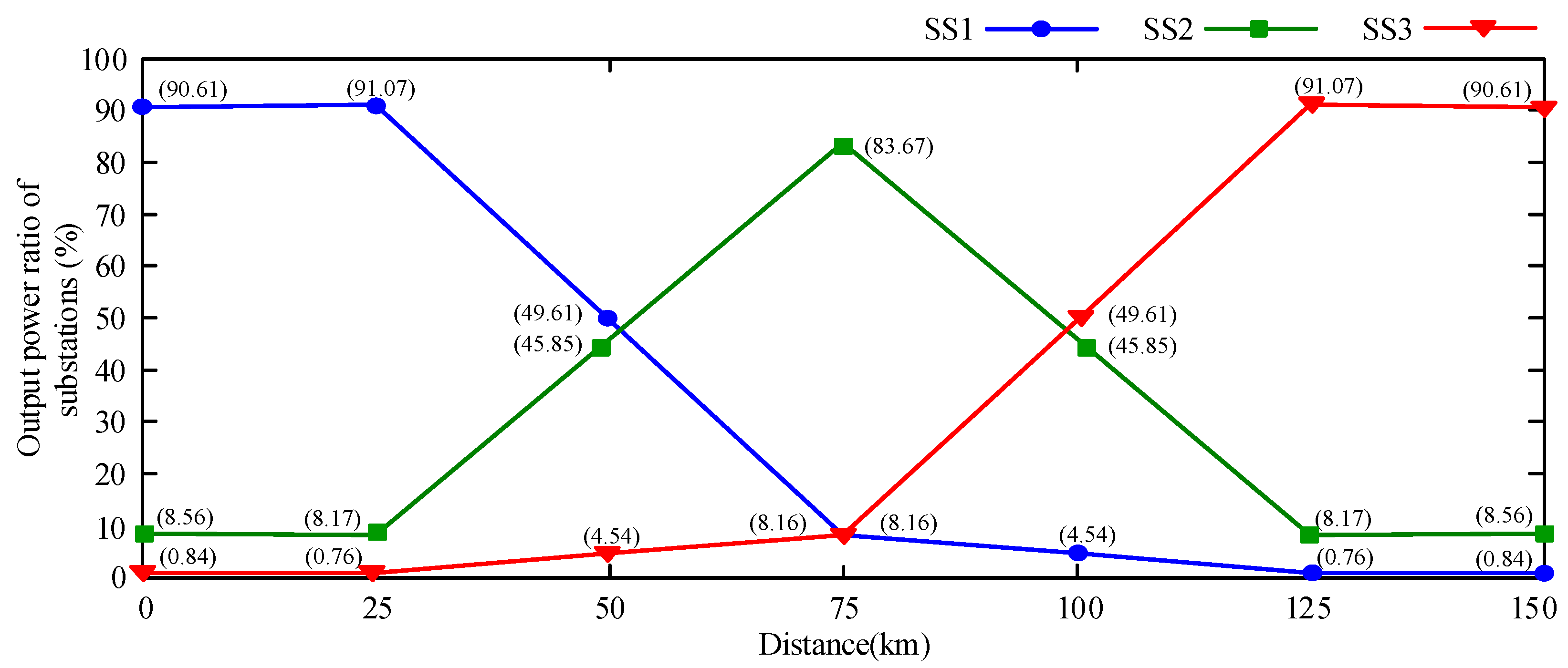
The simulation that sets three traction substations in the system is also achieved. In this simulation, the locomotive runs from the start (0 km) to the end (150 km). When the locomotive is at seven different locations, the output power of the traction substations are illustrated as shown in

Table 4. The output power of traction substations.

Distance	0 km	25 km	50 km	75 km	100 km	125 km	150 km
Traction substation 1	9.848	8.803	5.007	0.789	0.458	0.073	0.091
Traction substation 2	0.93	0.79	4.627	8.088	4.627	0.79	0.93
Traction substation 3	0.091	0.073	0.0458	0.789	5.007	8.803	9.848
Total	10.869	9.666	9.6798	9.666	10.092	9.666	10.869

.

Fitting the data of Table 4, the relationship between the distance and the output power ratio of each traction substation is expressed as Figure 11. It can be known by Figure 11 that the output power is varied with the change of the distance between the locomotive and the substation. Compared with the present traction substation, 10 percentages of the output power can be reduced by the traction substation of ACTPSS (approximately), which could have significant economic influence on the China railway system.

5. The Simulation Analysis and Experimental Verification

5.1. The Simulation Analysis of Three-Model Three-Phase to Single-Phase Cascaded Converter Based on ACTPSS

The simulation of the three-model three-phase to single-phase cascaded converter based on ACTPSS was built, and the feasibility of the control strategy and modulation strategy was verified. The simulation parameters are exhibited in

Table 5. The parameters of the three-model cascaded converter simulation.

Parameters	Value
The number of the cascaded model	3
The DC voltage of the single model	15 kV
The reference voltage of the traction network	27.5 kV
Power of the traction network	9.6 MW
The value of the capacitor in DC side	1 mF
The value of the fliter inductance	10 mH
The value of the fliter capacitor	10 μF
The carrier wave frequence of the inverter	1 kHz

.

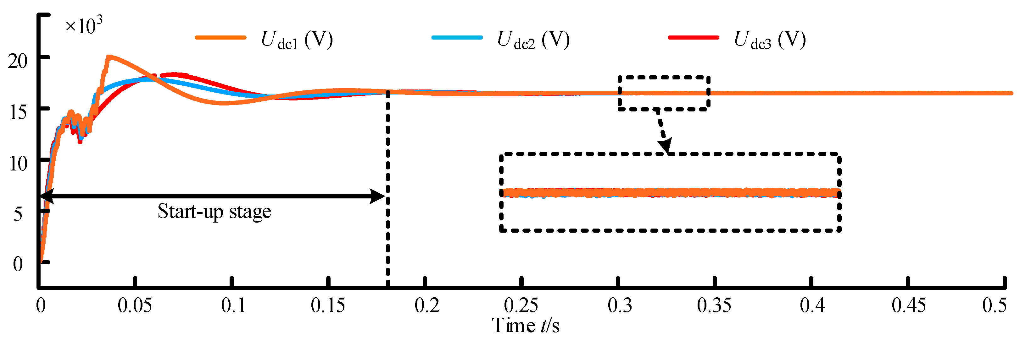
The output voltage waves of the three-phase 3L-NPC rectifiers are shown in Figure 12, and it can be known that the voltages could achieve stability after about 0.17 s. As the output waves appeared, the second-order ripple was suppressed by the LC filter. By the rectifiers, the steady and reliable DC voltages could be obtained.

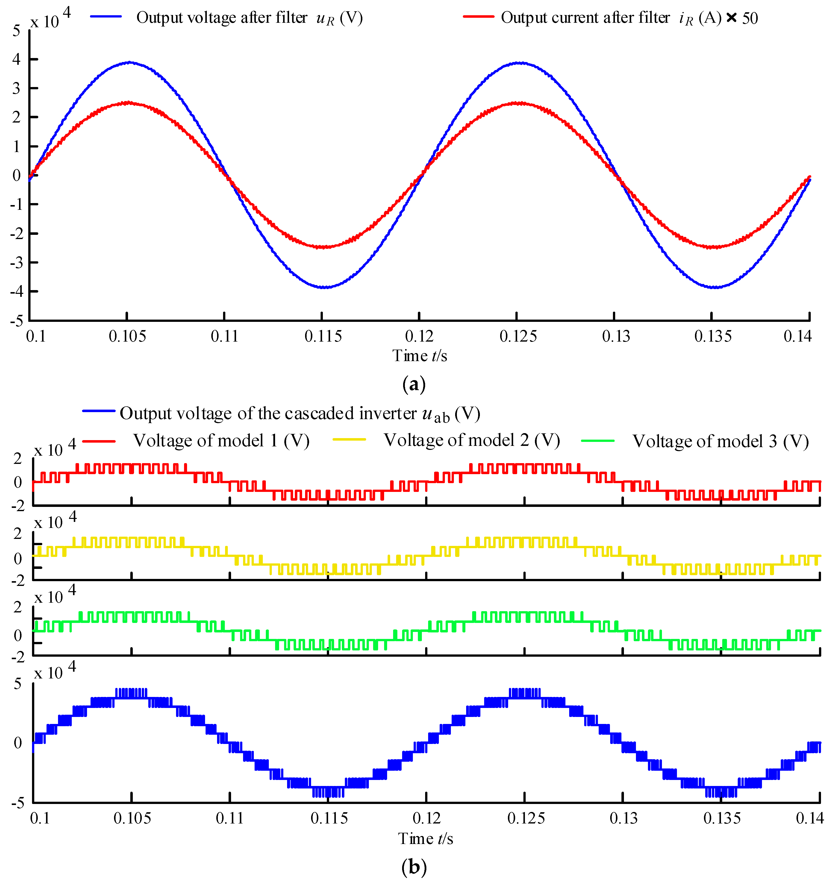
The output voltage and current waves of the three-model 3L-NPC cascaded inverter after filter are illustrated by Figure 13a. The u_R and i_R are the output voltage and current after the filter, respectively. In order to display the voltage and the current wave of output load properly and in the same scope, the current waveform was expanded by 50 times, the output voltage and current waveform were closed to the standard sine waves, and the output voltage that had little harmonic component and high power factor could be provided by the cascaded inverter. The 5-level output voltage waves of the three-inverter and the output voltage of the cascaded inverter are shown in Figure 13b. The u_ab is the 13-level output voltage of the three-model cascaded inverter, of which the effective value is 27.5 kV. The feasibility and availability of the cascaded inverter’s control strategy and modulation strategy have been verified by Figure 13.

5.2. The Simulation Analysis of ACTPSS

The simulation of ACTPSS was built, and three traction substations and three locomotives were set in this simulation. The locomotives worked as the traction load. The parameters of the system are illustrated in

Table 6. The parameters of ACTPSS.

Parameters	Value
The number of the traction substation	3
The reference voltage of the traction network	27.5 kV
The value of the fliter inductance in network side	10 mH
The value of the fliter capacitor in network side	10 μF
The carrier wave frequence of the inverter	1 kHz

.

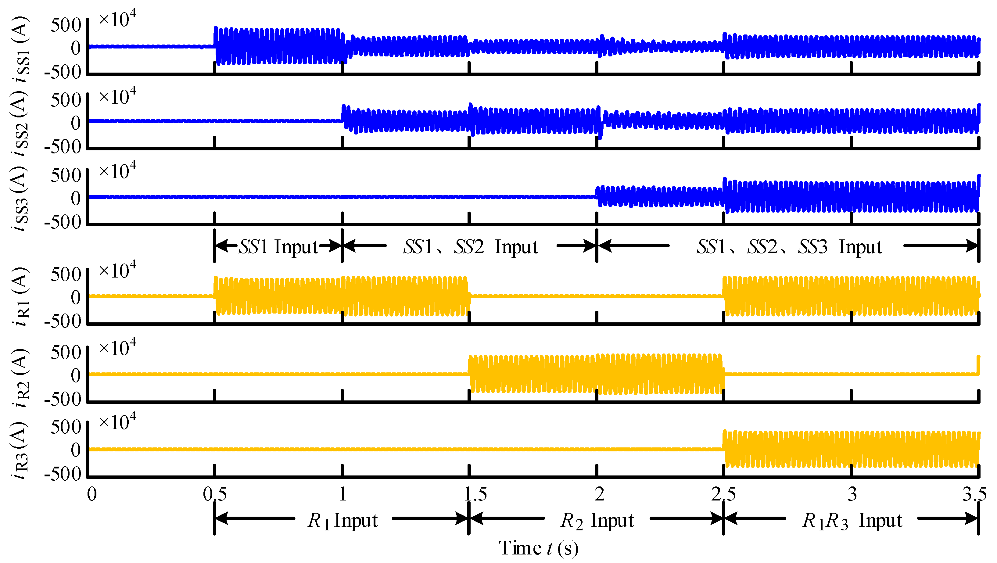
The locomotive 1 (R₁) was set to run in 0.5–1.5 s, 2.5–3.5 s, and 4.5–7 s in the simulation, the locomotive 2 (R₂) was set to run in 1.5–2.5 s and 3.5–6.0 s, while the locomotive 3 (R₃) was set to run in 2.5–5.0 s. The output current waves of the three traction substations and the current waves of the three locomotives are shown in Figure 14.

The traction substation 1 (SS1) was connected with the traction network at 0.5 s, the start of the system operation. The traction substation 2 (SS2) was connected with the traction network at 1.0 s, and the traction substation 3 (SS3) at 2.0 s. In 0.5–1.0 s, only the R₁ was under operation, and the power was provided to the R₁ only by the SS1, thus the current of the R₁ was the same as the current of the SS1 at this period. In 1.0–1.5 s, the power was supplied to the R₁ by both the SS1 and the SS2. In 1.5–2.0 s, only the R₂ was under operation, and the power was supplied to the R₂ by both the SS1 and the SS2. Because the distance between the R₂ and the SS2 was shorter, the power supplied by the SS2 was more than that supplied by the SS1. In 2.0–2.5 s, the power was supplied to the R₂ by the SS1, the SS2, and the SS3. Because the location of R₂ was between the SS2 and the SS3, the power provided by the SS1 was the least. In 2.5–3.0 s, the R₁ and the R₃ were under operation, and the power of them was supplied by the three traction substations together. At this period, the R₃ was on the right side of the SS3, and the power provided by the SS3 was more than that supplied by the SS1 and the SS2.

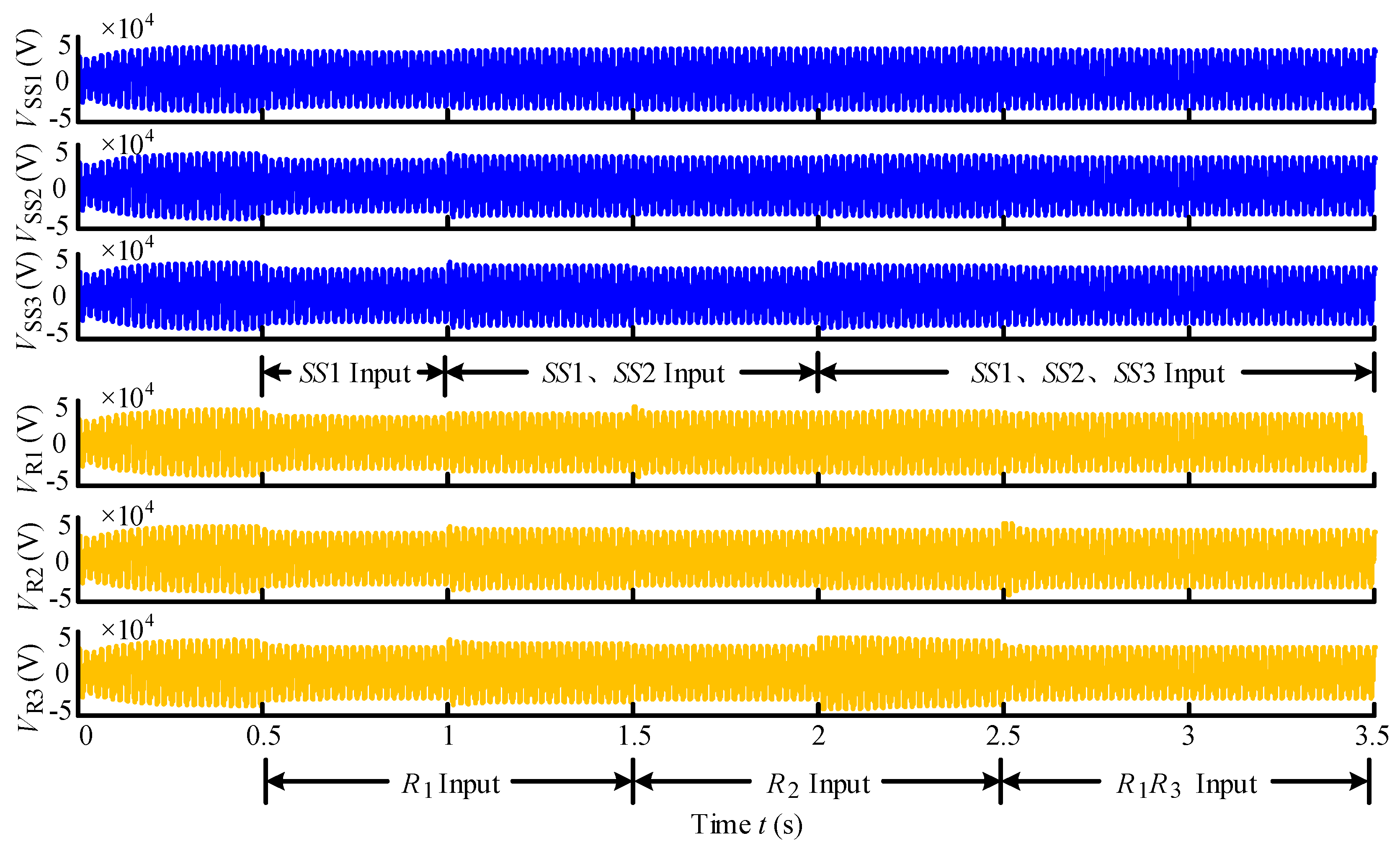
The output voltage waves of the traction substations and the voltage waves of locomotives in 0–3.5 s are exhibited in Figure 15. From the simulation results, it is clear that the output voltages of the traction substations and the voltages of locomotives were adjusted properly when the traction loads were input or excision. The voltages were maintained within the international prescribed scope, from 19 kV to 29 kV, ensuring that the locomotives could be under the normal operation.

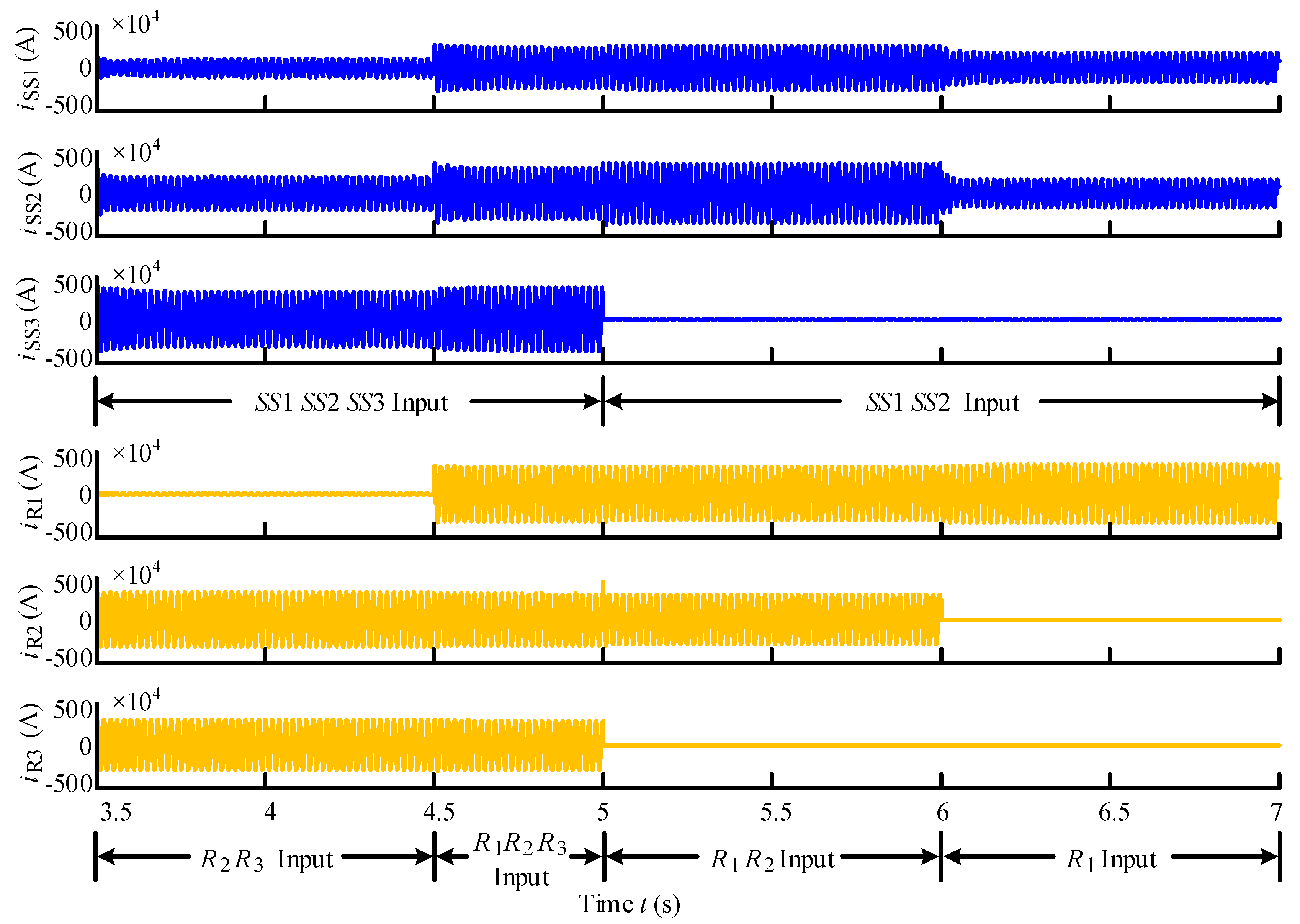
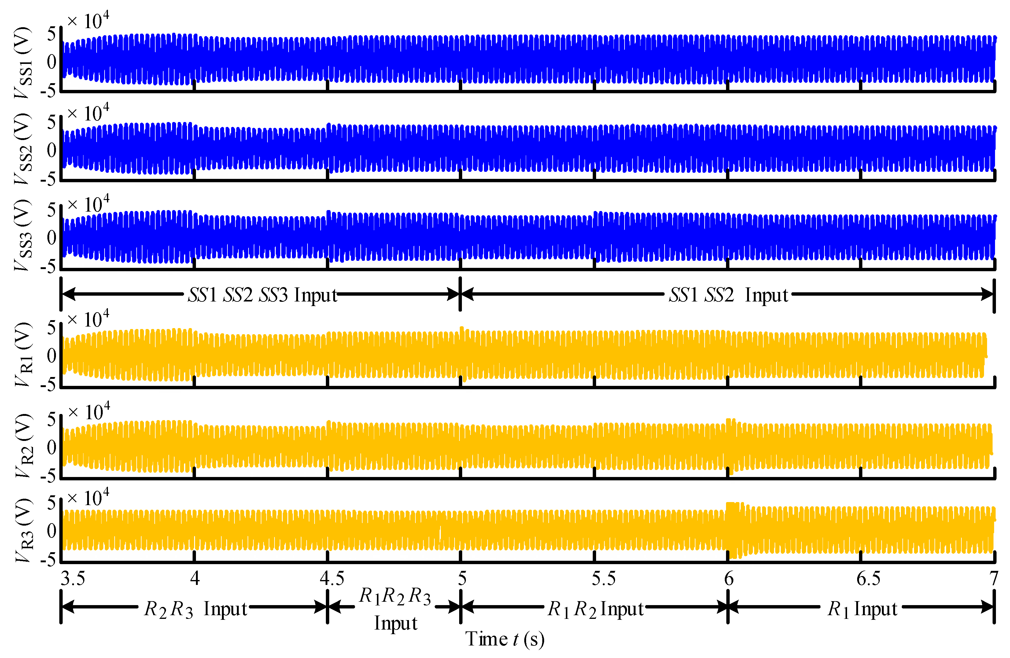
The output current waves of the traction substations and the current waves of locomotives in 3.5–7.0 s are exhibited in Figure 16. In 3.5–4.5 s, the R₂ and the R₃ were under operation, and the power of them was supplied by the three traction substation together. Because the distance between the R₂, the R₃, and the SS1 was longer, the power supplied by the SS1 was the least. In 4.5–5.0 s, the R₁, the R₂, and the R₃ were under operation, and the power of them was also provided by the three traction substations together. Because the R₃ was farther from the SS1 and the SS2 than from the SS3, the power supplied from the SS3 to the R₃ was the most. In 5.0–6.0 s, when the SS3 was excision because of fault, the R₁ and the R₂ were still under operation and obtained the power from the SS1 and the SS2. In 6.0–7.0 s, the R₁ was under operation and located between the SS1 and the SS2. The power was supplied to the R₁ by the SS1 and the SS2 equally.

The output voltage waves of the traction substations and the voltage waves of locomotives in 3.5–7.0 s are exhibited in Figure 17. From the simulation results, it is clear that the output voltages of the traction substations and the voltages of locomotives were adjusted properly when the traction loads were input or excision, and the voltages were maintained within the international prescribed scope, from 19 kV to 29 kV, ensuring that the locomotives could be under the normal operation.

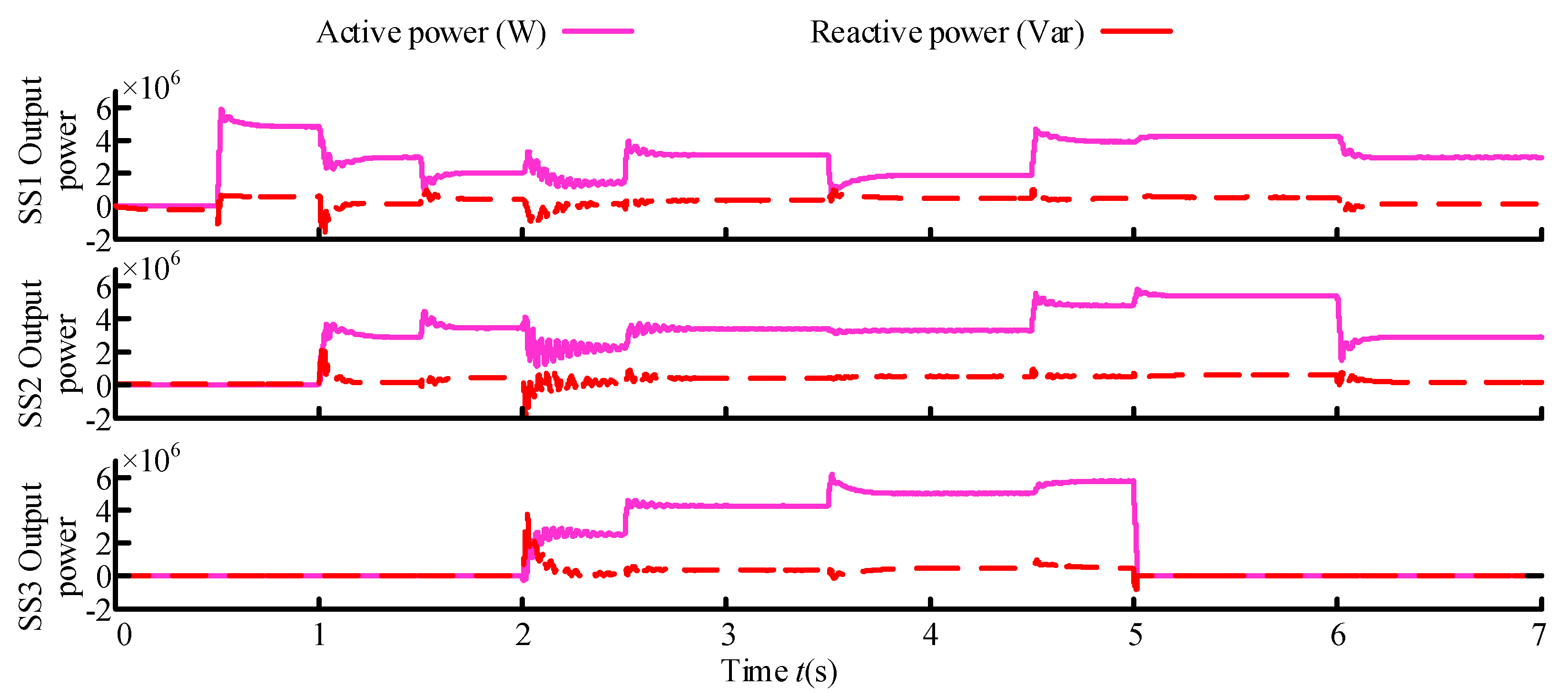
The output active and reactive power of the traction substations are illustrated by Figure 18. The converters inside the locomotives were controlled to operate with the unity power factor, thus the locomotives could be considered the pure resistance load. Therefore, under the steady operation of the locomotive, the reactive power was almost zero. When the locomotive started up or broke, the reactive power was outputted to achieve the power balance of the traction network.

5.3. The Exprimental Verification

The experimental platform of low power was built to verify the feasibility of the structure, control strategy, and modulation strategy. The platform consists of three parallel substations, which were composed of the three-model 3L-NPC cascaded converter.

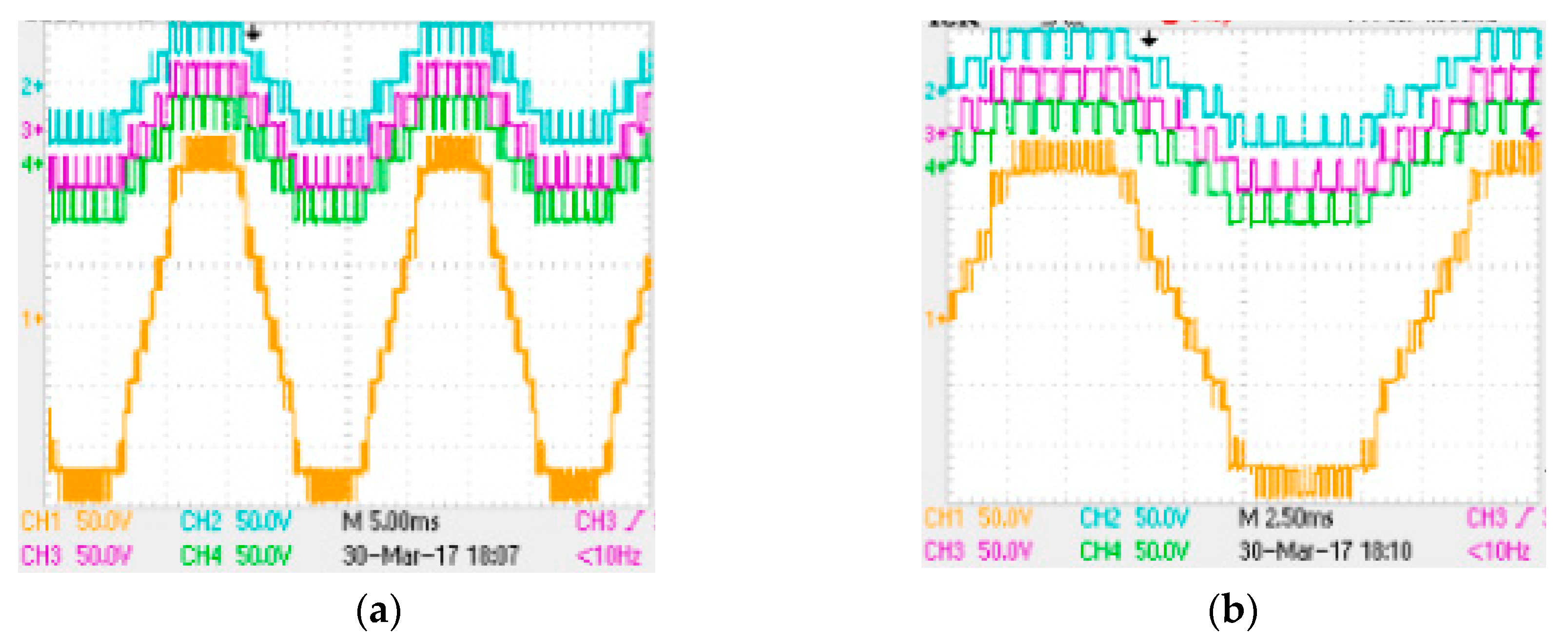
The output voltage waves of the three-model 3L-NPC cascaded converter are shown in Figure 19. Three 3L-NPC models were cascaded, thus the output voltage wave of each inverter was 5-level and the wave of the 3L-NPC cascaded converter was 13-level. The output voltage waves of the experiment were stable with the theoretical analysis.

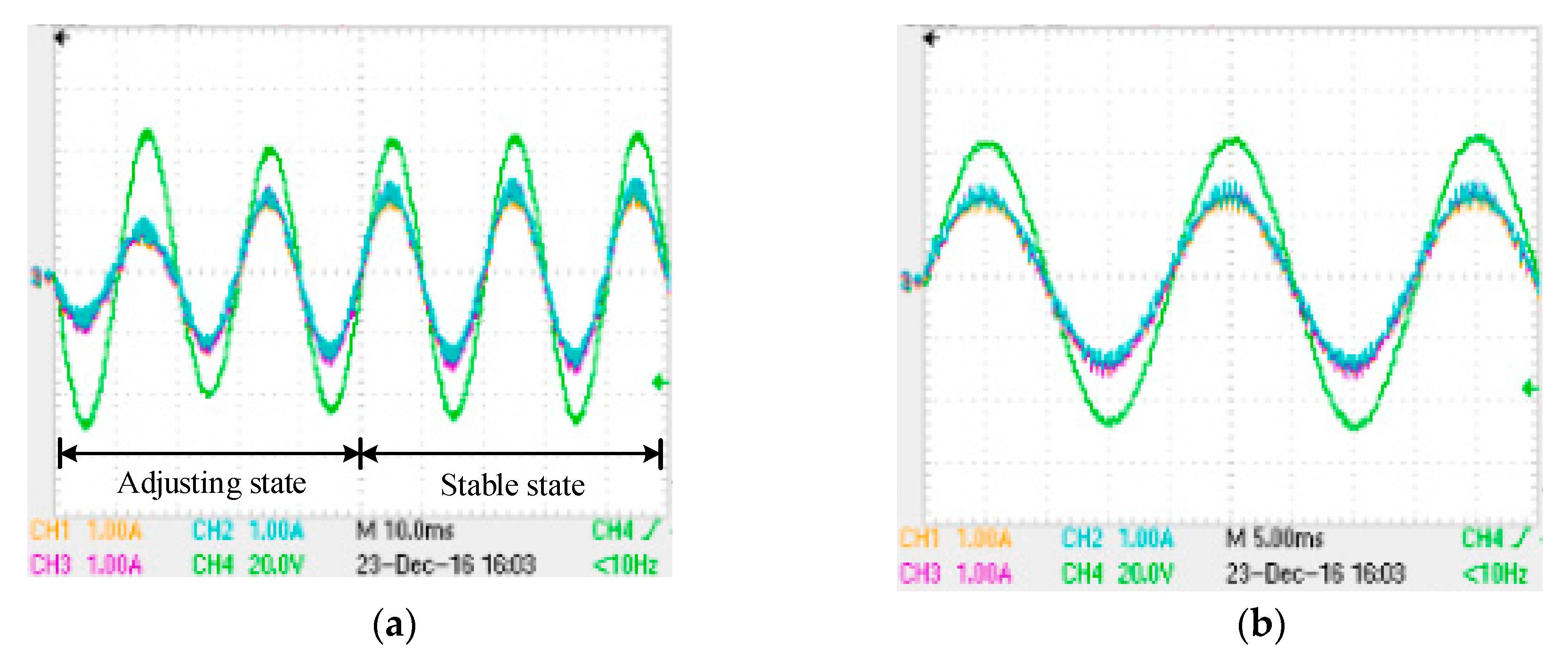
The output current waves of the three parallel traction substations and the load voltage wave are exhibited in Figure 20. The same amplitude and phase of three current waves were obtained after about 50 ms to adjust. The current could be outputted by three traction substations equally. The feasibility of the theoretical analysis and simulation could be verified by the results of the low power experiment.

6. Conclusions

In this paper, ACTPSS based on the three-phase to single-phase cascaded converter was studied to solve the problems of power qualities and to cancel all the neutral sections in traditional TPSS. Based on the research of ACTPSS, an improved PQ decomposition algorithm was proposed to calculate the power flow of ACTPSS. As a result, the impedance model of the traction network was built and analyzed. Then, the power flow situations under different operation conditions were analyzed. Finally, simulation and experimental results were given to validate the proposed improved PQ decomposition algorithm strategy. According to the aforementioned analysis and implementation, the following advantages could be obtained:

(1) The induced current in the rail-earth loop was far greater than that in the conduction circuit. As a result, when the distance between the locomotive and the substation was greater than 5 km, the resulting impedance calculation error was less than 5%. Therefore, the simplified equivalent model of the traction network was valid in the traction network impedance model of ACTPSS.

(2) The results showed that the minimum voltage of the traction network was higher than 19 kV, which met the running requirements of locomotive load. The analyses indicated that the capacity of the individual substation could be reduced by nearly 10%. The theoretical fundament of ACTPSS was laid in this paper.

(3) The power losses of the ACTPSS between the nodes were calculated. According to the calculation of the output power, the calculation results illustrated that the output power was affected by the distance between the locomotive and the traction substation. The closer the distance between the locomotive and the substation, the more power would output by the substation.

(4) On the basis of theoretical analysis, the correctness and validity of the proposed improved PQ decomposition algorithm strategy were proven by the simulation and the experimental, which laid a foundation for the application of ACTPSS.

References

- Feng, C.; Zhu, Q.; Yu, B.; Zhang, Y. Complexity and vulnerability of high-speed rail network in China. In Proceeddings of the 2017 36th Chinese Control Conference (CCC), Dalian, China, 26–28 July 2017; pp. 10034–10039. [Google Scholar]
- Zhang, J.; Wu, M.; Liu, Q. A Novel Power Flow Algorithm for Traction Power Supply Systems Based on the Thévenin Equivalent. Energies 2018, 11, 126. [Google Scholar] [CrossRef]
- Zhao, N.; Roberts, C.; Hillmansen, S.; Nicholson, G. A Multiple Train Trajectory Optimization to Minimize Energy Consumption and Delay. IEEE Trans. Intell. Transp. Syst. 2015, 16, 2363–2372. [Google Scholar] [CrossRef]
- Wang, H.; Li, Y.; Liu, H.; Wu, L.; Sun, Y. Transmission characteristics of harmonics and negative sequence components of electrified railway in power system. In Proceeddings of the 2016 International Conference on Smart Grid and Clean Energy Technologies (ICSGCE), Chengdu, China, 19–22 October 2016; pp. 301–306. [Google Scholar]
- Shu, Z.; Xie, S.; Lu, K.; Zhao, Y.; Nan, X.; Qiu, D.; Zhou, F.; Gao, S.; Li, Q. Digital detection, control, and distribution system for co-phase traction power supply application. IEEE Trans. Ind. Electron. 2013, 60, 1831–1839. [Google Scholar] [CrossRef]
- Yang, X.; Hu, H.; Ge, Y.; Aatif, S.; He, Z.; Gao, S. An Improved Droop Control Strategy for VSC-Based MVDC Traction Power Supply System. IEEE Trans. Ind. Appl. 2018, 54, 5173–5186. [Google Scholar] [CrossRef]
- He, X.; Guo, A.; Peng, X.; Zhou, Y.; Shi, Z.; Shu, Z. A Traction Three-Phase to Single-Phase Cascade Converter Substation in an Advanced Traction Power Supply System. Energies 2015, 8, 9915–9929. [Google Scholar] [CrossRef] [Green Version]
- Xie, B.; Zhang, Z.; Li, Y.; Hu, S.; Luo, L.; Rehtanz, C.; Krause, O. Reactive Power Compensation and Negative-Sequence Current Suppression System for Electrical Railways with YNvd-Connected Balance Transformer—Part II: Implementation and Verification. IEEE Trans. Power Electron. 2017, 32, 9031–9042. [Google Scholar] [CrossRef]
- Zhang, D.; Zhang, Z.; Wang, W.; Yang, Y. Negative Sequence Current Optimizing Control Based on Railway Static Power Conditioner in V/v Traction Power Supply System. IEEE Trans. Power Electron. 2016, 31, 200–212. [Google Scholar] [CrossRef]
- Li, Q.; Zhang, J.; He, W. Study of a new power supply system for heavy haul electric traction. J. China Railw. Soc. 1988, 10, 23–31. [Google Scholar]
- Zhang, R.; Lin, F.; Yang, Z.; Cao, H.; Liu, Y. A Harmonic Resonance Suppression Strategy for a High-Speed Railway Traction Power Supply System with a SHE-PWM Four-Quadrant Converter Based on Active-Set Secondary Optimization. Energies 2017, 10, 1567. [Google Scholar] [CrossRef]
- He, X.; Shu, Z.; Peng, X.; Zhou, Q.; Zhou, Y.; Zhou, Q.; Gao, S. Advanced Cophase Traction Power Supply System Based on Three-Phase to Single-Phase Converter. IEEE Trans. Power Electron. 2014, 29, 5323–5333. [Google Scholar] [CrossRef]
- Han, P.; He, X.; Wang, Yi.; Ren, H.; Peng, X.; Shu, Z. Harmonic Analysis of Single-Phase Neutral-Point-Clamped Cascaded Inverter in Advanced co-phase traction Power Supply System Based on the Big Triangular Carrier Equivalence Method. Energies 2017, 11, 1–16. [Google Scholar]
- Townsend, C.D.; Baraciarte, R.A.; Yu, Y.; Tormo, D.; Parra, H.Z.; Demetriades, G.D.; Agelidis, V.G. Heuristic Model Predictive Modulation for High-Power Cascaded Multilevel Converters. IEEE Trans. Ind. Electron. 2016, 63, 5263–5275. [Google Scholar]
- Haridas, K.; Khandelwal, S.; Das, A. Three phase to single phase modular multilevel converter using full bridge cells. Proceeddings of the 2016 IEEE International Conference on Power Electronics, Drives and Energy Systems (PEDES), Trivandrum, India, 14–17 December 2016; pp. 1–5. [Google Scholar]
- Lin, H.; Shu, Z.; He, X.; Liu, M. N-D SVPWM With DC Voltage Balancing and Vector Smooth Transition Algorithm for a Cascaded Multilevel Converter. IEEE Trans. Ind. Electron. 2018, 65, 3837–3847. [Google Scholar] [CrossRef]
- Plattner, G.; Semlali, H.F.; Kong, N. Analysis of probabilistic load flow using point estimation method to evaluate the quantiles of electrical networks state variables. CIRED Open Access Proc. J. 2017, 2017, 2087–2091. [Google Scholar] [CrossRef]
- Liu, H.; Tang, C.; Han, J.; Li, T.; Li, J.; Zhang, K. Probabilistic load flow analysis of active distribution network adopting improved sequence operation methodology. IET Gener. Trans. Distrib. 2017, 11, 2147–2153. [Google Scholar] [CrossRef]
- He, Z.; Hu, H.; Zhang, Y.; Gao, S. Harmonic Resonance Assessment to Traction Power-Supply System Considering Train Model in China High-Speed Railway. IEEE Trans. Power Deliv. 2014, 29, 1735–1743. [Google Scholar] [CrossRef]
- Hu, H.; Gao, S.; Shao, Y.; Wang, K.; He, Z.; Chen, L. Harmonic Resonance Evaluation for Hub Traction Substation Consisting of Multiple High-Speed Railways. IEEE Trans. Power Deliv. 2017, 32, 910–920. [Google Scholar] [CrossRef]
- Xu, S.; Miao, S. Calculation of TTC for multi-area power systems based on improved Ward-PV equivalents. IET Gen. Trans. Distrib. 2017, 11, 987–994. [Google Scholar] [CrossRef]
- Hu, S.; Xie, B.; Li, Y.; Gao, X.; Zhang, Z.; Luo, L.; Krause, O.; Cao, Y. A Power Factor-Oriented Railway Power Flow Controller for Power Quality Improvement in Electrical Railway Power System. IEEE Trans. Ind. Electron. 2017, 64, 1167–1177. [Google Scholar] [CrossRef]
- Madhusoodhanan, S.; Tripathi, A.; Patel, D.; Mainali, K.; Kadavelugu, A.; Hazra, S. Solid-State Transformer and MV Grid Tie Applications Enabled by 15 kV SiC IGBTs and 10 kV SiC MOSFETs Based Multilevel Converters. IEEE Trans. Ind. Appl. 2015, 51, 3343–3360. [Google Scholar] [CrossRef]
- Wang, C.; Xiao, L.; Zheng, X.; Lv, L.; Xu, Z.; Jiang, X. Analysis, Measurement, and Compensation of the System Time Delay in a Three-Phase Voltage Source Rectifier. IEEE Trans. Power Electron. 2016, 31, 6031–6043. [Google Scholar] [CrossRef]
- Jie, S.; Stefan, S.; Qu, B.; Zhang, Y.; Chen, K.; Zhang, R. Modulation Schemes for a 30-MVA IGCT Converter Using NPC H-Bridges. IEEE Trans. Ind. Appl. 2015, 51, 4028–4040. [Google Scholar]
- Li, Q.; He, J. Analysis of Traction Power Supply System; Southwest Jiaotong University Press: Chendu, China, 2012. [Google Scholar]
- Olsen, R.G.; Pankaskie, T.A. On the Exact, Carson and Image Theories for Wires at or Above the Earth’s Interface. IEEE Trans. Power Appar. Sys. 1983, PAS-102, 769–778. [Google Scholar] [CrossRef]
- Rao, L.; He, R.; Wang, Y.; Yan, W.; Bai, J.; Ye, D. An efficient improvement of modified Newton-Raphson algorithm for electrical impedance tomography. IEEE Trans. Magn. 1999, 35, 1562–1565. [Google Scholar]
Figure 1.
Traction power supply system. (left) The existing power supply substation, (right) the co-phase power supply substation based on active power compensators (APC).
Figure 2.
The structure of the advanced co-phase traction power supply system (ACTPSS).