Numerical Simulation on Interfacial Characteristics in Supersonic Steam–water Injector Using Particle Model Method


1
School of Energy and Power Engineering, Shandong University, Jinan 250061, Shandong, China
2
Jinan Drainage Management and Service Center, Jinan 250101, Shandong, China
*
Author to whom correspondence should be addressed.
Energies 2019, 12(6), 1108; https://0-doi-org.brum.beds.ac.uk/10.3390/en12061108
Submission received: 24 February 2019
/
Revised: 17 March 2019
/
Accepted: 20 March 2019
/
Published: 21 March 2019
(This article belongs to the Section I: Energy Fundamentals and Conversion)
Abstract
:Steam–water injectors have been widely applied in various industrial fields because of their compact and passive features. Despite its straightforward mechanical design, the internal two-phase condensing flow phenomena are extremely complicated. In present study, a numerical model has been developed to simulate steam–water interfacial characteristics in the injectors based on Eulerian–Eulerian multiphase model in ANSYS CFX software. A particle model is available for the interphase transfer between steam and water, in which a thermal phase change model was inserted into the model as a CFX Expression Language (CEL) to calculate interphase heat and mass transfer. The developed model is validated against a test case under a typical operating condition. The numerical results are consistent with experimental data both in terms of axial pressure and temperature profiles, which preliminarily demonstrates the feasibility and accuracy of particle model on simulation of gas–liquid interfacial characteristics in the mixing chamber of injector. Based on the dynamic equilibrium of steam supply and its condensation, interfacial characteristics including the variation of steam plume penetration length and steam–water interface have been discussed under different operating conditions. The numerical results show that steam plume expands with steam inlet mass flow rate and water inlet temperature increasing, while it contracts with the increase of water inlet mass flow rate and backpressure. Besides this, the condensation shock position moves upstream with the backpressure increasing.
1. Introduction
A steam–water injector (SI) is a pump-like device that consumes high-pressure steam to draw in cold water and raise its pressure. The most significant advantages of SI include the possible operation without external energy supply, rather compact make-up and lack of rotating machinery, resulting in a high operational reliability. The SI has been widely used in the industrial areas for district-heating system [1], Rankine cycle of steam power plants [2], and the passive safety systems of nuclear reactors [3,4,5,6,7,8,9,10]. The passive feature of SI has revived with more and more applications to passive core cooling systems, which can be used for high pressure makeup water supply in advanced light water reactors and high-pressure safety injection system for boiling water reactors. The SI could ensure the heat removal from a nuclear reactor core without electric power supply, fulfilling safety requirements. Besides, due to the efficient transfer of heat, mass and momentum in direct contact condensation (DCC) in mixing chamber, SI can also operate efficiently as direct contact feed water heaters [11].
The SI discussed in the presented study has a central steam jet configuration, i.e. central steam nozzle arrangement. The high-pressure steam serves as the motive medium while water is the entrained medium or suction medium. This injector type can operate with a low suction pressure [9] and reduce viscous dissipation as high-velocity steam and mixing chamber walls do not contact with each other [4,12]. The essence of SI is to increase the pressure of low-pressure fluid using high-pressure fluid without consuming mechanical energy. The SI consists of the following five main parts:
- 1.
- Steam nozzleIn steam nozzle, high-pressure steam will be accelerated to a supersonic velocity and create low pressure around the nozzle outlet which is below the pressure of suction water. If the steam inlet pressure is high enough, a converging–diverging nozzle (Laval type) should be adopted to ensure enough expansion, in case of expansion loss outside the nozzle.
- 2.
- Water nozzleThe suction water is taken in through a coaxial and annular conduit called water nozzle, whose function is to distribute the water evenly all around the steam nozzle exit.
- 3.
- Mixing chamberIn the mixing chamber, supersonic steam jet entrains water into the mixing chamber and contact directly with the suction water.
- 4.
- ThroatIn most cases, steam condenses completely in the vicinity of throat. This phenomenon, called condensation shock, causes a rapid pressure rise.
- 5.
- DiffuserDiffuser is a divergent channel with a single-phase flow inside. The flow is decelerated constantly, thus leading to a further increase of static pressure.
In the past decades, the SI study with respect to its application in nuclear power plants mainly focused on its attainable discharge pressure and operation behavior. SI can achieve optimum performance under stable working conditions. Cattadori et al. [4] tested an instrumented steam injector prototype and obtained a 10% higher discharge pressure than steam inlet pressure for core coolant makeup. Narabayashi et al. [8,9] concluded that SI could work in the high pressure range over 7 MPa, and discharged over 12 MPa. Deberne et al. [6] carried out visualized measurements on a transparent rectangular section and found that incomplete condensation could result in a decrease of the discharge pressure. Dumaz et al. [7] observed the condensation shock moves upstream with increase of discharge pressure based on the DEEPSSI project. By exergy analysis, Trela et al. [13] developed a procedure based on experimental data to evaluate exergy losses in SI parts and revealed that the highest irreversibility sources were in the two-phase region and in the steam nozzle. Kwidzinski [14] visually investigated condensation wave structure and concluded that SI can gain its best pressure-lift performance when condensation shock occurs at the end of mixing chamber.
Various numerical studies of SI have been conducted recently. Beithou and Aybar [3] proposed a mathematical model using one-dimensional control volume method for steam-driven jet pump. The calculated static pressure distributions were in good agreement with experimental results by Cattadori et al. [4]. Dumaz et al. [7] concluded that SI thermal-hydraulics can be described by the model based on the 1-D module of the system code CATHARE2, which could give the maximum backpressure within 10% of accuracy. Yan et al. [1] proposed a mathematical model to predict the pressure-lift performance. Shah et al. [10,11,15] proposed a model based on Eulerian two-phase flow model in conjunction with the realizable κ-ε turbulence model to investigate the characteristics of steam jet pump. The Lattice Boltzmann Method (LBM) method was also commonly used [16] because of its ability to capture multi-fluid physics including phase-change and interfacial dynamics with relative ease. Vinuesa et al. [17,18] employed a toolbox to compute turbulence statistics for high-fidelity simulations in flows of increasing complexity. Besides this, as a typical phenomenon in mixing chamber of SI, steam jet condensation into subcooled water in large space was studied by many researchers [19,20,21,22,23,24,25].
Restricted by experimental measuring methods [26,27,28,29], the details in internal steam–water interfacial behavior of SI is still unclear. The simulation still encounters some tough problems, whose major problem lies in the fact that the two-phase flow in mixing chamber is supercritical and extremely complicated. For these reasons, the motivation of the present work is to develop a valid and computationally efficient model to figure out the physical mechanism of DCC and provide new insights into the interfacial characteristics in SI. The novelty of the present model lies in the fact that a thermal phase change model was inserted into the particle model as a CFX Expression Language (CEL) to calculate interphase heat and mass transfer. Based on the numerical simulation, the presented results would help provide methods for the optimized design and safe operation of SI in related industrial applications.
2. Numerical Method
A numerical model based on Eulerian–Eulerian multiphase model has been used to simulate the heat and mass transfer characteristics of SI. Each phase has its separate set of conservation equations governing the equilibrium of mass, momentum and energy in the two-fluid model [30]. Particle model is available when one of the phases is continuous and the other is dispersed [31]. It is suitable for modeling dispersed multiphase flow cases, such as gas bubbles in a liquid, liquid droplets in a gas, and solid particles in a gas or liquid. In the present study, the particle model has been employed to calculate the interphase mass, momentum, and energy transfer, in which the primary and secondary phases is taken as continuous and dispersed phases, respectively. Liquid water denoted as α is the continuous phase and steam denoted as β is the dispersed phase.
2.1. Two-Fluid Model
The momentum equation for phase α can be expressed as
Since the phases α and β have the same form of conservation equations, only the equations of the phase α is shown in the model. SMα and Mα are the source terms from the external body force and interphase momentum transfer, respectively. Mα has been explained in detail in Section 2.3.3. r denotes volume fraction of steam in a cell. The effective dynamic viscosity μeffα contains molecular dynamic viscosity μα and turbulent dynamic viscosity μtα. The third term on the right of Equation (1) represents the momentum generated by interphase mass transfer.
The continuity equation for phase α:
Γαβ accounts for the interphase mass transfer rate due to condensation from phase β to α per unit volume.
The energy equation for phase α can be:
where eα, SEα, and Qα denote internal energy, the source term due to latent heat of condensation, and the energy source due to interphase heat transfer discussed in Section 2.3.2, respectively.
2.2. Turbulence Model
Dispersed phase zero equation model is used to describe the turbulence in gas side, which combines the turbulent kinematic viscosity of both phase α and β
where σ denotes a kind of turbulent Prandtl number taken as 1 in the model. The turbulent viscosity in the gas side can be acquired by that of liquid phase.
The standard k-ε model has been used for the liquid phase, and the k and ε equations can be:
Thus, the liquid turbulent viscosity is as follows
where Cμ, Cε1, Cε2, σk, and σε equal 0.09, 1.44, 1.92, 1.0, and 1.3, respectively. For supersonic flows, compressibility affects turbulence through so-called dilatation dissipation, which can be included in turbulence models [32]. In the present study, the compressibility effects on turbulence are considered in the k equation based on the Sarkar model [33].
2.3 Interphase Transfer Models
The condensation model based on thermal equilibrium has been used by many researchers [10,11,20,34,35,36,37] to investigate steam jet condensation or DCC in SI. The heat and mass transfer process can be divided into two steps: from steam to the interface and from the interface to liquid.
2.3.1. Interfacial Area
Interfacial transfer of mass, momentum and energy is directly dependent on the contact surface area between the two phases. The dispersed phase is treated as clusters of standard sphere particles. The interfacial area density is calculated by assuming that tiny gas bubbles is present as spherical particles in this study. The interfacial area per unit volume between phase α and phase β is
where dβ denotes the mean diameter of the spherical bubbles, and γβ is the gas volume fraction in the liquid phase.
2.3.2. Interphase Heat Transfer
The two-resistance model was used to calculate interphase heat transfer. As the interfacial condition is assumed to be saturated at the local steam pressure, the saturated temperature Tsat can be estimated by the fitted correlation in Equation (11).
The thermal resistance on gas side can be neglected, and the heat transfer coefficient is infinite. Thus, zero thermal resistance is assigned to gas side such that the temperature at the interface Tsat equals the gas phase temperature Tβ
The heat transfer rate per unit volume in liquid phase can be obtained as
where hα denotes heat transfer coefficient in liquid side, which can be calculated by
where Nuα can be obtained by Hughmark model; Nu, Re, and Pr are all estimated with properties of the liquid phase.
2.3.3. Interphase Momentum Transfer
For gas–liquid interphase momentum transfer in this model, drag force MDα, and turbulent dispersion force MTDα are considered. Drag force MDα is expressed as
where CD denotes drag force coefficient and can be included in Schiller Naumann drag force model:
Turbulent dispersion force can be calculated by Lopez de Bertodano model
where kα is turbulent kinetic energy, and CTD is turbulent dispersion force coefficient taken as 0.3.
2.3.4. Interphase Mass Transfer
The thermal phase change model [20] based on total heat flux equilibrium was inserted into particle model as a CFX Expression Language (CEL) to simulate interphase heat and mass transfer. The model describes the phase change induced by interphase heat transfer, which is only applicable for condensation or evaporation of pure substances. The sensible heat transfer rate per unit volume from the interface to the two phases can be:
As zero thermal resistance is assumed at the gas side, so the heat transfer rate qβ is zero. The total heat flux equilibrium was given by
where Γαβ denotes the rate of mass loss per interfacial area, Hβ denotes the steam specific enthalpy, HS is the specific enthalpy of water at interfacial temperature Tsat, which are regarded as interfacial values of enthalpy carried in and out of the phases due to phase change. Thus, the mass transfer rate from gas phase to liquid phase can be calculated by
3. Mesh Solution and Model Validation
3.1. Simulation Domain and Mesh Solution
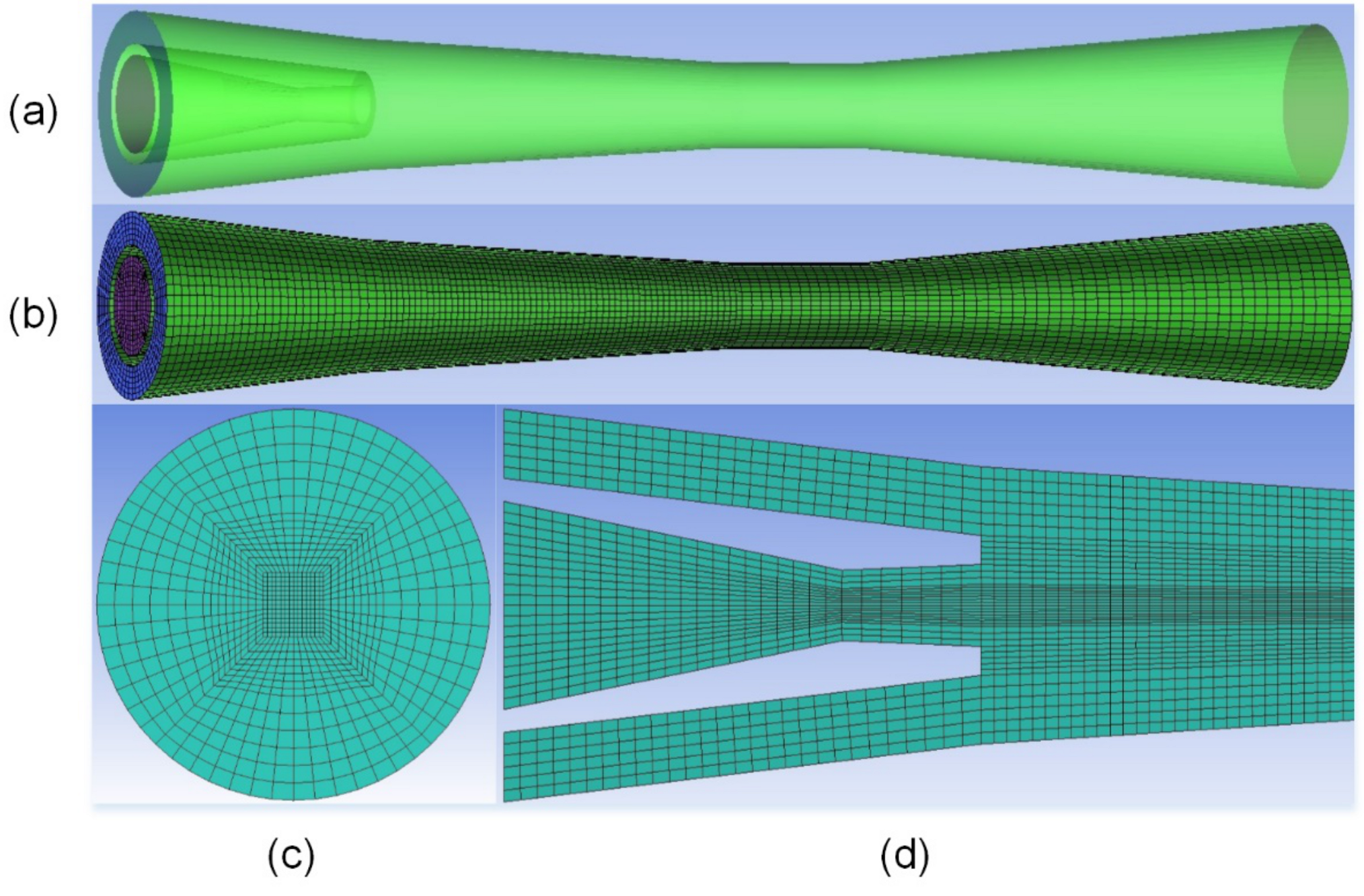
The presented numerical model for SI is compared against data from Shah’s experiment [15]. As shown in Figure 1, SI was composed of five parts: steam nozzle, water nozzle, mixing chamber, throat, and diffuser. The steam nozzle shape is Laval type. The water nozzle has been modified to a simplified form. All the parameters of geometric configuration are identical as that of Shah’s experiment. The 3-D fluid domain for simulation has been established, as shown in Figure 2a. The quality and density of mesh is the key factors of simulation convergence and accuracy. To achieve this goal, structural meshes for the fluid domain have been generated with O-block method using ANSYS ICEM. The overall blocks of the fluid domain in axial direction consists of three layers of O-blocks. The core of the O-blocks is a square block. The mesh is evenly distributed in the axial direction. Because of this reason, axisymmetric steam plume can be obtained. As shown in Figure 2b, denser and finer meshes are generated in mixing chamber and throat due to dramatic physical parameters change near the phasic interface. The representative mesh view in radial and axial section are shown in Figure 2c,d. The mesh quality is larger than 0.6, which can guarantee the calculation stability.
3.2. Boundary Conditions and Solver Settings
In the present simulation, appropriate boundary conditions are of vital significance to the final results. Mass flow rate inlet boundary conditions are adopted at the inlet of steam nozzle and water nozzle. Opening boundary condition with ambient entrainment pressure is assigned to the SI’s outlet and no-slip adiabatic condition is imposed on all walls’ boundaries.
A commercial software package CFX (Release 15.0, ANSYS Inc, Canonsburg, PA, USA) (Version, Manufacturer, City, State Abbr. if USA or Canada, Country) from ANSYS Technology was used. As the two-phase flow process in SI is highly turbulent, reaching supersonic, first-order upwind advection scheme was used for the discretization of conservation equations. The properties of water and steam including densities, thermal conductivity coefficient, specific heat capacity, viscosity, and specific enthalpy were taken from IAPWS-IF97 material group, which can be regarded as real gas model with high accuracies. Steady state analysis with double precision is available for the simulation. Convergence was achieved when RMS residuals of all equations fell below 10−4 and the monitored inlet pressure turned to be a constant value. A server with 44 CPU cores and 128 GB RAM was used for all the calculations. The details for solver control in the software are shown in Table 1.
3.3. Mesh Independency Check and Model Validation
For mesh independency check, the axial static pressure profiles along the SI centerline when mβ1 = 0.0102 kg/s, Tβ1 = 398 K, mα1 = 0.49 kg/s, Tα1 = 290 K was compared under three different mesh numbers of 95368, 142968, and 324976, respectively. As shown in Figure 3, when the numbers of mesh are 142968 and 324976, similar profiles of the axial static pressure are predicted. To ensure the calculation correctness and time-consuming expense, the middle number of cells, i.e., 142968 cells was chosen as the mesh solution.
In the numerical simulation, the boundary condition of steam inlet mass flow rate is enforced at the nozzle inlet. According to the theory of gas dynamics [38], the gas mass flow rate can be determined by Laval nozzle throat diameter and steam inlet parameters including its pressure and temperature in supersonic flow. The corresponding steam inlet pressure for different mass flow rates are shown in Table 2. The calculation results by Equation (24) indicate that when steam inlet flow rate is mβ1 = 0.0102 kg/s, the corresponding pressure is close to the experimental data Pβ1 = 220 kPa. The relationship of steam mass flow rate and its static pressure by CFX-Post method also demonstrates the same correspondence with that obtained by Equation (24). Thus, the boundary condition of steam inlet mass flow rate corresponds to the pressure inlet boundary.
where dt denotes Laval nozzle throat diameter, Pβ1 and ρβ1 are steam inlet pressure and density, respectively.
To ascertain the model accuracy, numerical results have been validated with corresponding experimental data [15]. The operating condition was set at mβ1 = 0.0102 kg/s, Tβ1 = 398 K, mα1 = 0.49 kg/s, Tα1 = 290 K, Pout = 96 kPa. As shown in Figure 4a, axial static pressure of both results shows good agreement with each other. For two-phase flow, the gas and liquid temperature can be acquired separately by ANSYS CFX-Post. Thus, a consolidated temperature of the two phases’ temperature is hard to obtain directly according to Ref. [36]. Figure 4b shows the axial temperature of experimental measuring points are distributed obviously between steam and water temperature profiles in two-phase flow region. Hence, the numerical results indicate that the current model can adequately predict the flow and heat transfer characteristics.
4. Results and Discussion
When steam is injected into subcooled water, a closed steam cavity called steam plume is formed at the nozzle outlet [39]. If steam inlet mass flux is high enough, reaching sonic and supersonic speed, the steam jet condensation is classified as stable condensation in the regime map [40]. For this case, the steam plume will exhibit a relatively stable shape, called stable steam plume. In the present study, supersonic steam jet condensation in the confined flow channel, i.e. mixing chamber, will form stable steam plume according to the above analysis.
The steam plume is continuously supplied by steam nozzle and condensed by the entrained water across the interface. Stable steam plume can be formed by the dynamic equilibrium between steam supply and its consumption, leading to an unchanged steam plume boundary. The amount of steam supply is represented by steam inlet mass flow rate, while the steam consumption rate is mainly condensed by the entrained water. The subcooled water inlet temperature and the inlet mass flow rate are used to show its condensation capacity. The steam supply and consumption rate will change with the variation of the steam and water inlet boundary conditions, making the fact that the steam plume has to adjust its boundary constantly to achieve a new dynamic equilibrium.
Steam plume can be evaluated by analyzing the steam volume fraction contours. The characteristic size of steam plume includes the maximum penetration length, which can mostly reflect the variation of steam plume volume. The steam plume shape obtained by the simulation is similar to the ones observed during steam jet condensation into subcooled water in large space [28,41,42,43] Furthermore, steam plume should be an emphasis of DCC in confined space, e.g. in SI, in case of thermal damage on heating walls.
Nine cases, covering the range of steam inlet mass flow rate (mβ1 = 0.0081–0.0102 kg/s), water inlet mass flow rate (mα1 = 0.38–0.49 kg/s), water inlet temperature (Tα = 290–310 K), and backpressure (Pout = 96–106 kPa), are performed to investigate the interfacial characteristics of supersonic two-phase flow in SI. The operating conditions in numerical simulation of all cases are shown in Table 3.
4.1. The Analysis of Axial Thermodynamic Parameters Profiles along the Centerline
Figure 5 shows the thermodynamic parameters along the SI centerline for case 3. As the Laval nozzle can produce nearly isentropic expansion and partially convert the enthalpy into kinetic energy, the steam temperature and pressure decrease rapidly, while the Mach number can go through a sharp rise simultaneously. The steam can be accelerated to the local sonic speed at the throat section, and the speed will be supersonic at nozzle exit. When the supersonic steam spurts out from the nozzle, the low-velocity liquid water is entrained into the mixing chamber, leading to violent interactions between the steam and water. In the DCC process, the two phases exchange mass, momentum, and energy across the phase interface. The steam Mach number will drop dramatically due to interfacial shear force, while the temperature rises in near-linear way and the static pressure is almost constant. Similar results were reported by other researchers [1,10]. Most of the condensation takes place almost instantaneously in the throat judging from the contour in Figure 5, meanwhile a rapid pressure rise indicates that the condensation shock occurs. The condensation shock can also account for the slight temperature lift at the end of mixing chamber. In the diffuser, the kinetic energy of single-phase water decreases for further increase of the discharge pressure.
Figure 6 displays steam velocity streamline in axial section for case 3. In mixing chamber, high-velocity steam jet flows upon the low-velocity entrained water, leading to the fact that radial steam velocity appears at the steam plume boundary due to the interfacial shear force. As a result, the velocity fields show a general wavy flow patterns across the steam–water interface, making violent momentum transfer with extremely turbulent flow between steam and water in DCC process. This phenomenon is in accordance with the experimental results by Xu et al. [44]. The steam velocity decreases sharply in the mixing chamber due to the wavy flow across the interface, which can explain the reason why the most significant exergy loss occurs in the two-phase flow region, i.e., mixing chamber and condensation shock [13].
4.2. Effect of Steam Inlet Mass Flow rate on Steam Volume Fraction and Mach Number Profiles
To investigate the effect of steam inlet mass flow rate, the other boundary conditions remain constant (mα1 = 0.49 kg/s, Tα1 = 290 K, Pout = 96 kPa). Figure 7a shows the variation of steam volume fraction at different steam inlet mass flow rates for case 1, 2, and 3, respectively. It can be observed that the whole fluid domain consists of four areas: steam plume, phase interface, two-phase mixing layer, and ambient water region. As the steam inlet mass flow rate increases from mβ1 = 0.0081 kg/s to 0.0102 kg/s, the steam plume maximum penetration lengthens and the steam–water interface area enlarges. The details of axial steam volume fraction variation is presented in Figure 7b, where X and r denote the axial location from steam nozzle inlet and steam volume fraction, respectively. When the initial steam flows through the Laval nozzle with isentropic expansion, the spontaneous condensation cannot be negligible. However, it can be treated as approximate single-phase flow, i.e., steam volume fraction kept nearly unchanged r = 1. When the high-velocity steam entrains and condenses upon the liquid water in mixing chamber, the axial steam volume fraction continues r = 1 state in steam plume region. Then, it undergoes a sharp decrease at the two-phase mixing layer and turns to r = 0 at the condensation terminus. Finally, the axial steam volume fraction r = 0 indicates single-phase liquid flow through the diffuser. The condensation terminus moves downstream with steam inlet mass flow rate increasing.
The trend can be explained by the fact that steam plume formation is controlled by the dynamic equilibrium of gas supply and the condensation of entrained water. At low steam inlet mass flow rate, steam condenses more quickly as compared to high steam inlet mass flow. As the steam inlet mass flow rate mβ1 increases, the additional supplied steam exceeds the condensation capacity of water. In order to condense more amount of steam, the steam plume has to enlarge its boundary to enhance the condensation rate in the liquid side. Therefore, the steam plume travels longer distance with the increase of steam inlet mass flow rate.
In supersonic SI, Mach number is an important parameter. The maximum Mach numbers at the Laval nozzle outlet at different steam inlet mass flow rates are shown in Table 4, which are 1.184, 1.203, and 1.273 for case 1, case 2, and case 3, respectively. The results demonstrate that the Laval nozzle designed in such a way can accelerate the motive steam to supersonic value. Figure 8 depicts the contours of Mach number in axial section for case 3 and the centerline steam velocity at different steam inlet mass flow rates. The steam velocity at the Laval nozzle outlet is higher than 600 m/s for mβ1 = 0.0102 kg/s, which can create lower pressure to produce stronger suction effect. The maximum steam velocity achieved at the Laval nozzle outlet rises with steam inlet mass flow rate increasing.
4.3. Effect of Water Inlet Temperature on Steam Volume Fraction
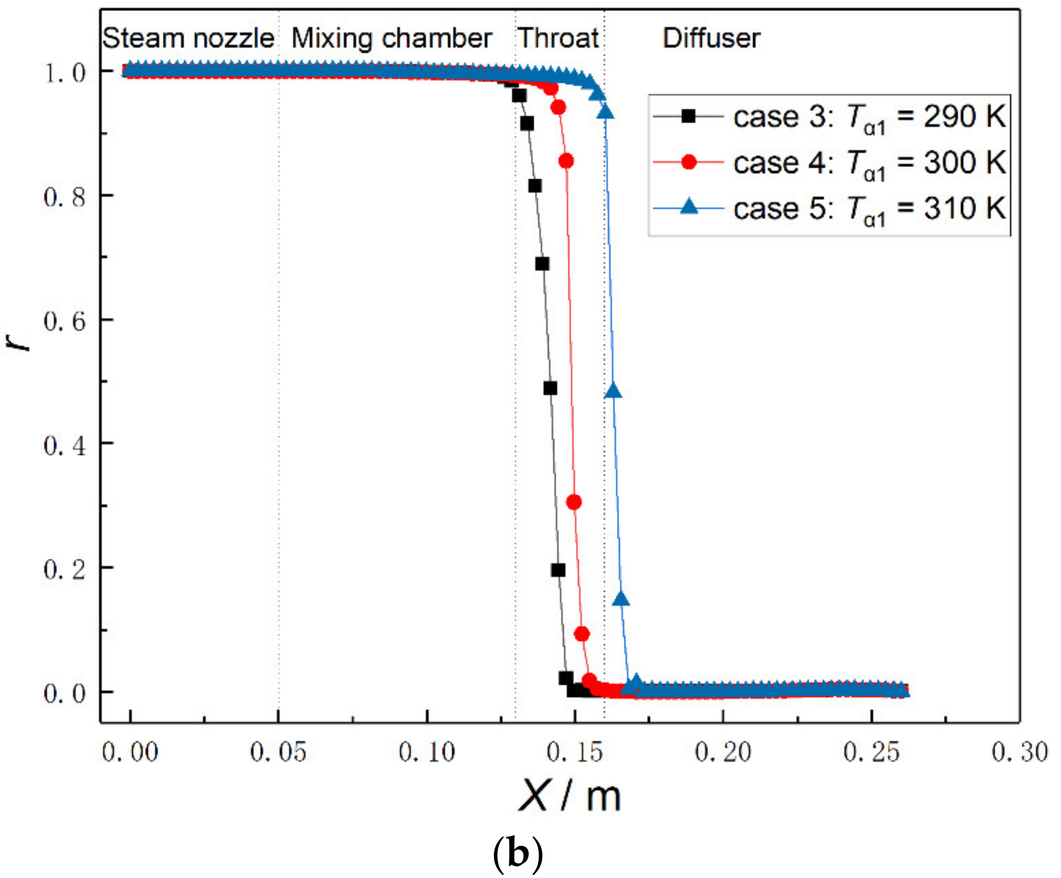
As illustrated in Figure 9a, as water inlet temperature increases from 290 K to 310 K, the steam plume penetration stretches for longer distance and the steam–water interface expands. Figure 9b describes a detailed comparison to evaluate the variation of axial steam volume fraction along SI centerline at different water inlet temperatures Tα1. As Tα1 increases from 290 K to 310 K, the condensation terminus moves downstream along the flow direction.
Based on the equilibrium of gas supply and condensation consumption, this can be explained by the fact that when the supplied steam is fixed, the total heat flux across the interface should be unchanged. As the entrained water inlet temperature rises, the temperature difference of condensation heat transfer between the interface and subcooled water decreases, which results in the fact that the condensation capacity of water will decline correspondingly and the steam could not be condensed immediately after being injected into the mixing chamber, so the steam plume reaches a new equilibrium by enlarging its interface area to condense the same amount of steam. As a result, the steam plume penetrates longer distance and expands with the increase of water inlet temperature due to the decrease of the condensation capability of water. However, the temperature difference between the steam and water at mixing chamber inlet has significant influence on the SI work and flow stability. With the rise of water inlet temperature, the decreasing temperature difference shifts the condensation terminus towards the diffuser with fixed backpressure, as shown in Figure 9a. According to Ref. [14], SI can attain its best pressure-lift performance when the condensation shock occurs at the end of mixing chamber. Therefore, the flow stability and the optimum performance is hard to obtain with high water inlet temperature.
4.4. Effect of Water Inlet Mass Flow Rate on Steam Volume Fraction
Steam plume shape is not only affected by the steam mass flow rate and water temperature, but water mass flow rate also plays an important role. Figure 10a shows the influence of water inlet mass flow rate on the steam volume fraction in axial section. The steam plume penetration slightly shortens and the steam–water interface contracts with water inlet flow rate increasing. Figure 10b shows a comparison to evaluate the variation of axial steam volume fraction along SI centerline at different water inlet mass flow rates. As the water mass flow rate increases from mα1 = 0.38 kg/s to 0.49 kg/s, the condensation terminus moves upstream slightly judging from the enlarged view in Figure 10b.
The interphase mass transfer accompanies the momentum and energy transfer, which complicates the transport phenomena. Therefore, an accurate calculation of the mass transfer is required to properly model the transport phenomena. As described in Section 2.3.4, the thermal phase change model based on total heat flux equilibrium [20] takes care of the interphase mass transfer, in which the condensation mass source term is defined using CFX Expression Language. The contours of mass transfer rate in axial section for case 3 is presented in Figure 11. The results show that interphase mass transfer takes place along the whole gas–liquid interface between the two phases. In addition, the maximum mass transfer rate locates at the tail of steam plume, i.e., condensation terminus. By comparing axial condensation rate profiles along the centerline at different water inlet mass flow rates, the condensation rate increases with water inlet mass flow rate increasing.
This phenomenon can be explained from the viewpoint of heat flux equilibrium determined by gas supply and condensation. As the supplied steam is fixed, i.e. a constant heat flux in the gas side, the total heat flux across the interface should be unchanged. With the increase of water inlet mass flow rate, the turbulence intensity increases, which will enhance heat transfer in the liquid side. As a result, the condensation capacity of water will become stronger as demonstrated in Figure 11 and the steam is quickly condensed after being injected into the mixing chamber, leading to the fact that the steam plume comes to a new equilibrium by reducing its interface area to condense the same amount of steam. Therefore, for a certain steam mass flow rate, the heat transfer interfacial area decreases with water inlet mass flow rate increasing due to the enhanced heat transfer in the liquid side.
4.5. Effect of Backpressure on Steam Volume Fraction and Condensation Shock Position
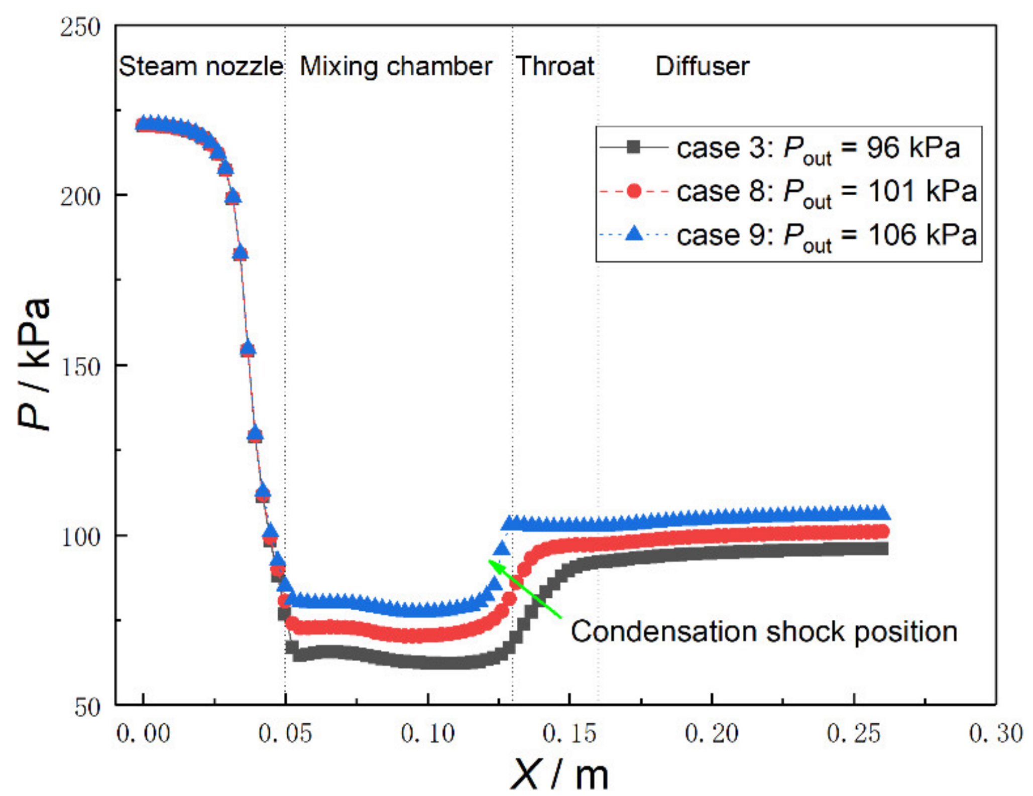
The outlet pressure of SI is called backpressure, denoted as Pout. The effect of backpressure on steam volume fraction was investigated. As shown in Figure 12a, the steam plume penetration shortens and the interface shrinks with backpressure increasing from Pout = 96 kPa to 106 kPa. Figure 12b shows a comparison to evaluate the variation of axial steam volume fraction along SI centerline at different backpressures. The condensation terminus moves upstream as Pout increases from 96 kPa to 106 kPa.
Condensation shock is the typical physical phenomenon in supersonic flow. As the inlet conditions of steam and water parameters are fixed, the comparison of axial static pressure profiles along the centerline at different backpressures is depicted in Figure 13. In general, the vanishing position of gas phase is associated with the generation of condensation shock. By comparing Figure 12 and Figure 13, a rapid pressure increase appears right in the vicinity of condensation terminus, which is regarded as condensation shock position. When the backpressure of SI is relatively low (i.e. 96 kPa means the SI open to ambient atmosphere), the condensation shock locates in the farthest position apart from the mixing chamber inlet. It is observed that the condensation shock position moves upstream with the backpressure increasing from 96 kPa to 106 kPa, changing simultaneously with corresponding condensation terminus. This phenomenon is in accordance with the experimental results by Dumaz et al. [7].
5. Conclusions
A numerical model has been developed based on Eulerian–Eulerian multiphase model to simulate the effect of operating conditions on the steam–water contact condensation in SI, in which particle model is used to calculate interphase mass, momentum, and energy transfer due to the interfacial complexity between steam and water. The influences of steam mass flow rate, water temperature, water mass flow rate, and backpressure on interfacial characteristics have been discussed. The main conclusions are summarized as follows:
- (1)
- The axial thermodynamic parameters along SI centerline including static pressure, Mach number, and temperature are used to analyze the overall physical process of SI. The maximum Mach number achieved at the Laval nozzle outlet rises with steam inlet mass flow rate increasing and the interphase momentum transfer is enhanced by the wavy flow across the steam–water interface according to the streamline.
- (2)
- Based on the equilibrium of steam supply and its condensation, interfacial characteristics including the variation of steam plume penetration length and the steam–water interface have been discussed under different operating conditions. The simulation results show that steam plume penetration lengthens and the steam–water interface expands with steam inlet mass flow rate and water inlet temperature increasing, while steam plume penetration shortens and the interface contracts with the increase of water inlet mass flow rate and backpressure.
- (3)
- Combined with the contour of steam volume fraction, the condensation shock position moves upstream with the backpressure increasing, changing simultaneously with corresponding condensation terminus.
Author Contributions
Methodology, X.C.; Software, X.C.; Data Curation, X.C.; Writing—Original Draft Preparation, X.C.; Supervision, M.T. and G.Z.; Funding Acquisition, M.T.; References Collection, H.L.
Funding
This work was supported by the National Natural Science Foundation of China (Nos. 51676114, 51576115 and 51806128), the China Postdoctoral Science Foundation (No. 2018M642655) and the Shandong Provincial Natural Science Foundation (No. ZR2016EEM26).
Conflicts of Interest
The authors declare no conflict of interest.
Nomenclatures
| Aαβ | interfacial area per unit volume (1/m) |
| dβ | gas bubble diameter (mm) |
| D | kinematic diffusion coefficient |
| e | internal energy (J) |
| h | heat transfer coefficient (W/(m2·K)) |
| k | turbulent kinetic energy (J) |
| Hs | saturation enthalpy of liquid phase at interfacial temperature (J/kg) |
| Hβ | saturation enthalpy of gas phase (J/kg) |
| m | mass flow rate (kg/s) |
| Mα | source term due to momentum transfer |
| Nu | Nusselt number |
| P | static pressure (kPa) |
| Pr | Prandtl number |
| Qα | sensible heat flux from interface to liquid phase (W/m2) |
| Qβ | sensible heat flux from gas to interface (W/m2) |
| r | steam volume fraction |
| Re | Reynolds number |
| Sc | Schmidt number |
| SMα | source term from external body force |
| T | static temperature (K) |
| Tsat | saturated steam temperature at local pressure (K) |
| w | mass fraction |
| X | axial location from nozzle inlet (m) |
| Subscript | |
| α | liquid phase |
| β | gas phase |
| t | Laval nozzle throat |
| out | steam–water injector outlet |
| 1 | steam nozzle or water nozzle inlet |
| Greek symbols | |
| μ | dynamic viscosity (Pa·s) |
| ρ | volume-averaged density (kg/m3) |
| Γ | interphase mass transfer (kg/(m3·s)) |
| κ | adiabatic index |
| Acronyms | |
| SI | steam–water injector |
| DCC | direct contact condensation |
References
- Yan, J.-J.; Shao, S.-F.; Liu, J.-P.; Zhang, Z. Experiment and analysis on performance of steam-driven jet injector for district-heating system. Appl. Therm. Eng. 2005, 25, 1153–1167. [Google Scholar] [CrossRef]
- Trela, M.; Kwidziński, R.; Głuch, J.; Butrymowicz, D. Analysis of application of feed-water injector heaters to steam power plants. Pol. Marit. Res. 2009, 16, 64–70. [Google Scholar] [CrossRef]
- Beithou, N.; Aybar, H.S. A mathematical model for steam-driven jet pump. Int. J. Multiph. Flow 2000, 26, 1609–1619. [Google Scholar] [CrossRef]
- Cattadori, G.; Galbiati, L.; Mazzocchi, L.; Vanini, P. A single-stage high pressure steam injector for next generation reactors: Test results and analysis. Int. J. Multiph. Flow 1995, 21, 591–606. [Google Scholar] [CrossRef]
- Deberne, N.; Leone, J.F.; Duque, A.; Lallemand, A. A model for calculation of steam injector performance. Int. J. Multiph. Flow 1999, 25, 841–855. [Google Scholar] [CrossRef]
- Deberne, N.; Leone, J.-F.; Lallemand, A. Local measurements in the flow of a steam injector and visualisation. Int. J. Therm. Sci. 2000, 39, 1056–1065. [Google Scholar] [CrossRef]
- Dumaz, P.; Geffraye, G.; Kalitvianski, V.; Verloo, E.; Valisi, M.; Méloni, P.; Achilli, A.; Schilling, R.; Malacka, M.; Trela, M. The DEEPSSI project, design, testing and modeling of steam injectors. Nucl. Eng. Des. 2005, 235, 233–251. [Google Scholar] [CrossRef]
- Narabayashi, T.; Mizumachi, W.; Mori, M. Study on two-phase flow dynamics in steam injectors. Nucl. Eng. Des. 1997, 175, 147–156. [Google Scholar] [CrossRef]
- Narabayashi, T.; Mori, M.; Nakamaru, M.; Ohmori, S. Study on two-phase flow dynamics in steam injectors: II. High-pressure tests using scale-models. Nucl. Eng. Des. 2000, 200, 261–271. [Google Scholar] [CrossRef]
- Shah, A.; Chughtai, I.R.; Inayat, M.H. Experimental and numerical analysis of steam jet pump. Int. J. Multiph. Flow 2011, 37, 1305–1314. [Google Scholar] [CrossRef]
- Shah, A.; Chughtai, I.R.; Inayat, M.H. Experimental and numerical investigation of the effect of mixing section length on direct-contact condensation in steam jet pump. Int. J. Heat Mass Trans. 2014, 72, 430–439. [Google Scholar] [CrossRef]
- Yan, J.; Wu, X.; Chong, D.; Liu, J. Experimental Research on Performance of Supersonic Steam-Driven Jet Injector and Pressure of Supersonic Steam Jet in Water. Heat Trans. Eng. 2011, 32, 988–995. [Google Scholar] [CrossRef]
- Trela, M.; Kwidzinski, R.; Butrymowicz, D.; Karwacki, J. Exergy analysis of two-phase steam–water injector. Appl. Therm. Eng. 2010, 30, 340–346. [Google Scholar] [CrossRef]
- Kwidzinski, R. Experimental investigation of condensation wave structure in steam–water injector. Int. J. Heat Mass Trans. 2015, 91, 594–601. [Google Scholar] [CrossRef]
- Shah, A. Thermal Hydraulic Analysis of Steam Jet Pump. Ph.D. Thesis, Pakistan Institute of Engineering and Applied Sciences, Islamabad, Pakistan, 2012. [Google Scholar]
- Kähler, G.; Bonelli, F.; Gonnella, G.; Lamura, A. Cavitation inception of a van der Waals fluid at a sack-wall obstacle. Phys. Fluids 2015, 27, 123307(1)–123307(26). [Google Scholar] [CrossRef]
- Vinuesa, R.; Fick, L.; Negi, P.; Marin, O.; Merzari, E.; Schlatter, P. Turbulence Statistics in a Spectral Element Code: A Toolbox for High-Fidelity Simulations; Argonne National Lab.: Argonne, IL, USA, 2017; 14p. [Google Scholar]
- Rezaeiravesh, S.; Vinuesa, R.; Liefvendahl, M.; Schlatter, P. Assessment of uncertainties in hot-wire anemometry and oil-film interferometry measurements for wall-bounded turbulent flows. Eur. J. Mech. Fluids 2018, 72, 57–73. [Google Scholar] [CrossRef]
- Dahikar, S.K.; Sathe, M.J.; Joshi, J.B. Investigation of flow and temperature patterns in direct contact condensation using PIV, PLIF and CFD. Chem. Eng. Sci. 2010, 65, 4606–4620. [Google Scholar] [CrossRef]
- Gulawani, S.S.; Dahikar, S.K.; Mathpati, C.S.; Joshi, J.B.; Shah, M.S.; RamaPrasad, C.S.; Shukla, D.S. Analysis of flow pattern and heat transfer in direct contact condensation. Chem. Eng. Sci. 2009, 64, 1719–1738. [Google Scholar] [CrossRef]
- Gulawani, S.S.; Joshi, J.B.; Shah, M.S.; RamaPrasad, C.S.; Shukla, D.S. CFD analysis of flow pattern and heat transfer in direct contact steam condensation. Chem. Eng. Sci. 2006, 61, 5204–5220. [Google Scholar] [CrossRef]
- Heinze, D.; Schulenberg, T.; Behnke, L. A physically based, one-dimensional three-fluid model for direct contact condensation of steam jets in flowing water. Int. J. Heat Mass Trans. 2017, 106, 1041–1050. [Google Scholar] [CrossRef]
- Norman, T.L.; Revankar, S.T. Jet-plume condensation of steam–air mixtures in subcooled water, Part 1: Experiments. Nucl. Eng. Des. 2010, 240, 524–532. [Google Scholar] [CrossRef]
- Choo, Y.J.; Song, C.-H. PIV measurements of turbulent jet and pool mixing produced by a steam jet discharge in a subcooled water pool. Nucl. Eng. Des. 2010, 240, 2215–2224. [Google Scholar] [CrossRef]
- Wu, X.-Z.; Yan, J.-J.; Li, W.-J.; Pan, D.-D.; Chong, D.-T. Experimental study on sonic steam jet condensation in quiescent subcooled water. Chem. Eng. Sci. 2009, 64, 5002–5012. [Google Scholar] [CrossRef]
- Zong, X.; Liu, J.-P.; Liu, J.; Yang, X.-P.; Yan, J.-J. Experimental study on the interfacial behavior of stable steam jet condensation in a rectangular mix chamber. Int. J. Heat Mass Trans. 2017, 114, 458–468. [Google Scholar] [CrossRef]
- Zong, X.; Liu, J.-P.; Yan, J.-J. Experimental study on the interfacial wave and local heat transfer coefficient of stable steam jet condensation in a rectangular mix chamber. Int. J. Heat Mass Trans. 2018, 127, 1096–1101. [Google Scholar] [CrossRef]
- Zong, X.; Liu, J.-P.; Yang, X.-P.; Yan, J.-J. Experimental study on the direct contact condensation of steam jet in subcooled water flow in a rectangular mix chamber. Int. J. Heat Mass Trans. 2015, 80, 448–457. [Google Scholar] [CrossRef]
- Shah, A.; Chughtai, I.R.; Inayat, M.H. Experimental study of the characteristics of steam jet pump and effect of mixing section length on direct-contact condensation. Int. J. Heat Mass Trans. 2013, 58, 62–69. [Google Scholar] [CrossRef]
- Ishii, M.; Hibiki, T. Thermo-Fluid Dynamics of Two-Phase Flow; Springer US: New York, USA, 2006; pp. 119–128. [Google Scholar]
- ANSYS®. Academic Research, Release 150, Help System, ANSYS CFX-Solver Theory Guide; ANSYS Inc: Canonsburg, PA, USA, 2013. [Google Scholar]
- Bonelli, F.; Viggiano, A.; Magi, V. A Numerical Analysis of Hydrogen Underexpanded Jets Under Real Gas Assumption. J. Fluids Eng. 2013, 135, 121101. [Google Scholar] [CrossRef]
- Sarkar, S.; Balakrishnan, L. Application of a Reynolds-Stress Turbulence Model to the Compressible Shear Layer. AIAA J. 1991, 29, 743–749. [Google Scholar] [CrossRef]
- Shah, A.; Chughtai, I.R.; Inayat, M.H. Numerical Simulation of Direct-contact Condensation from a Supersonic Steam Jet in Subcooled Water. Chin. J. Chem. Eng. 2010, 18, 577–587. [Google Scholar] [CrossRef]
- Zhou, L.; Chong, D.; Liu, J.; Yan, J. Numerical study on flow pattern of sonic steam jet condensed into subcooled water. Ann. Nucl. Energy 2017, 99, 206–215. [Google Scholar] [CrossRef]
- Qu, X.-H.; Sui, H.; Tian, M.-C. CFD simulation of steam–air jet condensation. Nucl. Eng. Des. 2016, 297, 44–53. [Google Scholar] [CrossRef]
- Qu, X.-H.; Tian, M.-C.; Zhang, G.-M.; Leng, X.-L. Experimental and numerical investigations on the air–steam mixture bubble condensation characteristics in stagnant cool water. Nucl. Eng. Des. 2015, 285, 188–196. [Google Scholar] [CrossRef]
- Maurice, J.Z.; Joe, D.H. Gas Dynamics; Wiley: Hoboken, NJ, USA, 1976; Volume 1. [Google Scholar]
- Qiu, B.; Yan, J.; Liu, J.; Chong, D.; Zhao, Q.; Wu, X. Experimental investigation on the second dominant frequency of pressure oscillation for sonic steam jet in subcooled water. Exp. Therm. Fluid Sci. 2014, 58, 131–138. [Google Scholar] [CrossRef]
- Cho, S.; Song, C.H.; Park, C.K.; Yang, S.K.; Chung, M.K. Experimental study on dynamic pressure pulse in direct contact condation of steam jets discharging into subcooled water. In Proceedings of the 1st Korea-Japan Symposium on Nuclear Thermal Hydraulics and Safety, Pusan, Korea, 21–24 October 1998. [Google Scholar]
- Qiu, B.; Tang, S.; Yan, J.; Liu, J.; Chong, D.; Wu, X. Experimental investigation on pressure oscillations caused by direct contact condensation of sonic steam jet. Exp. Therm. Fluid Sci. 2014, 52, 270–277. [Google Scholar] [CrossRef]
- Qiu, B.; Yan, J.; Liu, J.; Chong, D. Experimental investigation on pressure oscillation frequency for submerged sonic/supersonic steam jet. Ann. Nucl. Energy 2015, 75, 388–394. [Google Scholar] [CrossRef]
- Xu, Q.; Guo, L.; Zou, S.; Chen, J.; Zhang, X. Experimental study on direct contact condensation of stable steam jet in water flow in a vertical pipe. Int. J. Heat Mass Trans. 2013, 66, 808–817. [Google Scholar] [CrossRef]
- Xu, Q.; Guo, L.; Chang, L.; Wang, Y. Velocity field characteristics of the turbulent jet induced by direct contact condensation of steam jet in crossflow of water in a vertical pipe. Int. J. Heat Mass Trans. 2016, 103, 305–318. [Google Scholar] [CrossRef]
Figure 1.
Schematic and principal dimensions of steam–water injector (SI) from Shah’s experiment [15] (all dimensions are in mm).
Figure 1.
Schematic and principal dimensions of steam–water injector (SI) from Shah’s experiment [15] (all dimensions are in mm).

Figure 2.
Simulation domain and mesh. (a) Schematic model of simulation domain; (b) Overall geometry showing external surface mesh; (c) Local mesh detail in radial section; (d) Local denser mesh in axial section of steam nozzle and mixing chamber.
Figure 2.
Simulation domain and mesh. (a) Schematic model of simulation domain; (b) Overall geometry showing external surface mesh; (c) Local mesh detail in radial section; (d) Local denser mesh in axial section of steam nozzle and mixing chamber.

Figure 3.
Mesh independency check, mβ1 = 0.0102 kg/s, Tβ1 = 398 K, mα1 = 0.49 kg/s, Tα1 = 290 K.

Figure 4.
Comparison of axial static pressure and temperature profiles between numerical result and experimental data, mβ1 = 0.0102 kg/s, Tβ1 = 398 K, mα1 = 0.49 kg/s, Tα1 = 290 K, Pout = 96 kPa. (a) axial static pressure profile; (b) axial temperature profile.
Figure 4.
Comparison of axial static pressure and temperature profiles between numerical result and experimental data, mβ1 = 0.0102 kg/s, Tβ1 = 398 K, mα1 = 0.49 kg/s, Tα1 = 290 K, Pout = 96 kPa. (a) axial static pressure profile; (b) axial temperature profile.

Figure 5.
Axial profiles of static pressure, Mach number, and temperature for case 3.

Figure 6.
Steam velocity streamline in axial section for case 3.

Figure 7.
Effect of steam inlet mass flow rate mβ1 on steam volume fraction. (a) Contours of steam volume fractions at different steam inlet mass flow rates; (b) Axial profiles of steam volume fractions at different steam inlet mass flow rates.
Figure 7.
Effect of steam inlet mass flow rate mβ1 on steam volume fraction. (a) Contours of steam volume fractions at different steam inlet mass flow rates; (b) Axial profiles of steam volume fractions at different steam inlet mass flow rates.

Figure 8.
Contours of Mach number in axial section for case 3 and axial profiles of steam velocities at different steam inlet mass flow rates.
Figure 8.
Contours of Mach number in axial section for case 3 and axial profiles of steam velocities at different steam inlet mass flow rates.

Figure 9.
Effect of water inlet temperature Tα1 on steam volume fraction. (a) Contours of steam volume fractions at different water inlet temperatures; (b) Axial profiles of steam volume fractions at different water inlet temperatures.
Figure 9.
Effect of water inlet temperature Tα1 on steam volume fraction. (a) Contours of steam volume fractions at different water inlet temperatures; (b) Axial profiles of steam volume fractions at different water inlet temperatures.


Figure 10.
Effect of water inlet mass flow rate mα1 on steam volume fraction. (a) Contours of steam volume fractions at different water inlet mass flow rates; (b) Axial profiles of steam volume fractions at different water inlet mass flow rates.
Figure 10.
Effect of water inlet mass flow rate mα1 on steam volume fraction. (a) Contours of steam volume fractions at different water inlet mass flow rates; (b) Axial profiles of steam volume fractions at different water inlet mass flow rates.

Figure 11.
Contours of interphase mass transfer rate for case 3 and axial profiles of interphase mass transfer rates at different water inlet mass flow rates.
Figure 11.
Contours of interphase mass transfer rate for case 3 and axial profiles of interphase mass transfer rates at different water inlet mass flow rates.

Figure 12.
Effect of backpressure Pout on steam volume fraction. (a) Contours of steam volume fractions at different backpressures; (b) Axial steam volume fraction profiles along the centerline at different backpressures.
Figure 12.
Effect of backpressure Pout on steam volume fraction. (a) Contours of steam volume fractions at different backpressures; (b) Axial steam volume fraction profiles along the centerline at different backpressures.

Figure 13.
Axial static pressure profiles along the centerline at different backpressures.


Table 1.
Discretization scheme and Interpolation type.
| Variable | Method |
|---|---|
| Advection scheme | Upwind |
| Turbulence numerics | First order |
| Pressure interpolation type | Linear-linear |
| Velocity interpolation type | Linear-linear |
| Velocity pressure coupling | Second-order |
Table 2.
The relationship between steam inlet mass flow rate and corresponding pressure for different calculation methods.
Table 2.
The relationship between steam inlet mass flow rate and corresponding pressure for different calculation methods.
| mβ1 (kg/s) | Pβ1 in Exp. (kPa) | Pβ1 by gas dynamics (kPa) | Pβ1 in CFX-Post (kPa) |
|---|---|---|---|
| 0.0081 | 180 | 181 | 179 |
| 0.0092 | 200 | 206 | 198 |
| 0.0102 | 220 | 222 | 221 |
Table 3.
Operating conditions in numerical simulation.
| Case No. | mβ1 (kg/s) | Tβ1 (K) | mα1 (kg/s) | Tα1 (K) | Pout (kPa) |
|---|---|---|---|---|---|
| case 1 | 0.0081 | 390 | 0.49 | 290 | 96 |
| case 2 | 0.0092 | 394 | 0.49 | 290 | 96 |
| case 3 | 0.0102 | 398 | 0.49 | 290 | 96 |
| case 4 | 0.0102 | 398 | 0.49 | 300 | 96 |
| case 5 | 0.0102 | 398 | 0.49 | 310 | 96 |
| case 6 | 0.0102 | 398 | 0.38 | 290 | 96 |
| case 7 | 0.0102 | 398 | 0.43 | 290 | 96 |
| case 8 | 0.0102 | 398 | 0.49 | 290 | 101 |
| case 9 | 0.0102 | 398 | 0.49 | 290 | 106 |
Table 4.
The maximum Mach numbers at different steam inlet mass flow rates.
| Case No. | mβ1 (kg/s) | Mamax |
|---|---|---|
| case 1 | 0.0081 | 1.184 |
| case 2 | 0.0092 | 1.203 |
| case 3 | 0.0102 | 1.273 |
© 2019 by the authors. Licensee MDPI, Basel, Switzerland. This article is an open access article distributed under the terms and conditions of the Creative Commons Attribution (CC BY) license (http://creativecommons.org/licenses/by/4.0/).
Share and Cite
MDPI and ACS Style
Chen, X.; Tian, M.; Zhang, G.; Liu, H. Numerical Simulation on Interfacial Characteristics in Supersonic Steam–water Injector Using Particle Model Method. Energies 2019, 12, 1108. https://0-doi-org.brum.beds.ac.uk/10.3390/en12061108
AMA Style
Chen X, Tian M, Zhang G, Liu H. Numerical Simulation on Interfacial Characteristics in Supersonic Steam–water Injector Using Particle Model Method. Energies. 2019; 12(6):1108. https://0-doi-org.brum.beds.ac.uk/10.3390/en12061108
Chicago/Turabian StyleChen, Xianbing, Maocheng Tian, Guanmin Zhang, and Houke Liu. 2019. "Numerical Simulation on Interfacial Characteristics in Supersonic Steam–water Injector Using Particle Model Method" Energies 12, no. 6: 1108. https://0-doi-org.brum.beds.ac.uk/10.3390/en12061108
Note that from the first issue of 2016, this journal uses article numbers instead of page numbers. See further details here.