An Augmented Prony Method for Power System Oscillation Analysis Using Synchrophasor Data

Abstract

Intrinsic mode functions (IMFs) provide an intuitive representation of the oscillatory modes and are mainly calculated using Hilbert–Huang transform (HHT) methods. Those methods, however, suffer from the end effects, mode-mixing and Gibbs phenomena since they use an iterative procedure. This paper proposes an augmented Prony method for power system oscillation analysis using synchrophasor data obtained from a wide-area measurement system (WAMS). In the proposed method, in addition to the estimation of the modal information, IMFs are extracted using a new explicit mathematical formulation. Further, an indicator based on an energy and phase relationship of IMFs is proposed, which allows system operators to recognize the most effective generators/actuators on specific modes. The method is employed as an online oscillation-monitoring framework providing inputs for the so-called wide-area damping control (WADC) module. The efficacy of the proposed method is validated using three test cases, in which the IMFs calculation is simpler and more accurate if compared with other methods.

1. Introduction

Power system oscillation analysis has received considerable attention over the past decades. Features such as frequency and damping of the power system oscillations provide critical information for system operators [1]. Analysis of such oscillations are conducted using: (i) model-based and (ii) measurement-based approaches. The former approach is based on the linearized differential equation of the system around a specific operating point [2,3], as accurate modeling of power systems for various operating conditions is complicated and these approaches may not be useful for practical applications. On the other hand, with developing phasor measurement units (PMUs) and wide-area measurement system (WAMS), the latter approach became more popular. Recently, several studies have attempted to extract oscillation parameters using synchrophasor data. Some of the well-known methods used for oscillation detection using measurement-based approaches include: Kalman Filter (KF) [4] estimation of signal parameters by rotational invariance technique (ESPRIT) [5], Hilbert–Huang transform (HHT) [6,7,8,9], Yule–Walker algorithm [10], wavelet transform (WT) [11], recursive adaptive stochastic subspace identification (RASSI) [12], maximum likelihood method [13], and Prony analysis method [14,15,16]. Among them, the Prony method is one of the most commonly used measurement-based methods. The Prony method can directly estimate modal components of a measured signal. Recently, extensions of the Prony method have been developed that can calculate oscillatory modes of multiple signals in a central [14] or distributed [15] manner. Furthermore, a forward and backward extended Prony (FBEP) method is proposed in order [16] to reduce the sensitivity of the Prony method to noise.

A practical online oscillation monitoring framework should be able to determine the power system oscillations fast and accurately. Further, it should be capable of identifying contributions of different system buses in each oscillatory mode. Among the above methods, only the HHT method can determine the contribution of each state variable in various oscillatory modes. In general, each state variable of the system can be expressed as the sum of exponential sinusoids. According to the HHT method, each of the exponential sinusoids is called intrinsic mode functions (IMF). Using IMFs, participation of each system bus in an oscillatory mode can be determined by means of an indicator called node contribution factor (NCF). In the HHT method, IMFs can be extracted from the synchrophasor data using empirical mode decomposition (EMD), which is an iterative procedure. However, EMD process has some inherent shortcomings such as the end effects (EEs), mode-mixing and Gibbs phenomena. Some of those drawbacks have been addressed in improved versions of the HHT method in [6,7,8,9].

In this paper, we propose an augmented Prony based framework for real-time power system oscillation monitoring and analysis using synchrophasor data. The proposed framework estimates modal features (i.e., its damping and frequency) of a measured signal, while it is capable of determining contributions of different system buses in oscillatory modes by calculating IMFs and NCFs. Note that in the proposed framework, IMFs and thus NCFs are extracted using an explicit mathematical formulation based on an augmented Prony method. To the best of the authors’ knowledge, the Prony method has never been used before for the calculation of IMFs and thus NCFs. Unlike the HHT method that relies on heuristic approaches such as EMD for the calculation of IMFs, in the proposed approach they are calculated using an explicit mathematical formulation, which is one of the novelties of the proposed method. The calculation of IMFs in the proposed framework is more accurate, while it requires a lower computational burden if compared to the existing HHT methodologies. The proposed online oscillation-monitoring framework can be used as an input for the so-called wide-area damping control (WADC) module, which is responsible for controlling the system oscillations. Note that obtaining NCFs associated with oscillatory modes in the system can assist power system operators to take better remedial actions enhancing system stability and security. The effectiveness of the proposed framework is validated using the Kundur’s two-area test system and a practical power system. The main innovative contributions in this paper are:

○

A novel augmented Prony-based oscillation analysis method is proposed for smart systems with WAMS.

○

A novel explicit mathematical formulation is proposed for online obtaining IMFs and NCFs.

○

A new IMF-based method for determining the effective order of the system is also suggested.

○

The proposed method can eliminate the negative effects of EE, Gibbs, and mode-mixing which are the main challenges in previous methods such as HHT.

○

The proposed NCF can help system operators to recognize the most effective generators/actuators on a specific mode in the system.

The rest of the paper is organized as follows: the motivations behind the work and the formulations IMFs and NCFs calculation in the proposed framework are presented in Section 2. In Section 3, performance of the proposed framework is analyzed using the Kundur’s two-area power system and a practical power system. Finally, Section 4 concludes the paper.

2. Proposed Framework for WAMS-Based Oscillation Detection

2.1. Research Motivation

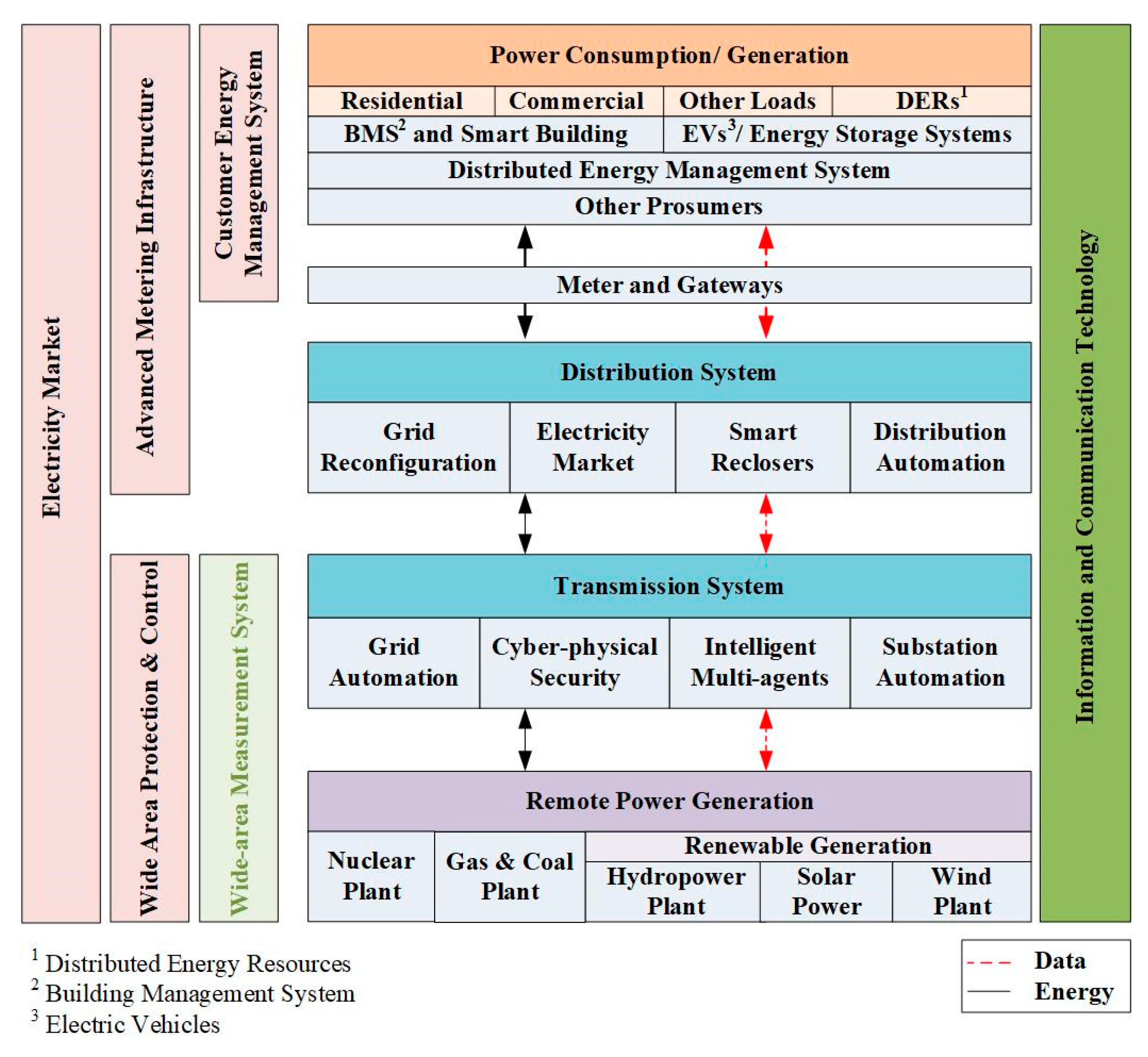
Developing a real-time power system oscillation monitoring framework is an important part of small signal stability studies using WAMS technologies. An overview of Smart Grid components and technologies is shown in Figure 1. Observe that the smart grid consists of different state-of-the-art technologies enabling effective network management schemes in the presence of renewable energy systems, flexible loads, and energy storage systems. This new concept ultimately offers the efficient and reliable operation of future power systems via a two-way exchange of data and energy among different sectors in the electric power supply chainmn including generation, transmission, distribution, and consumption. Implementation of PMUs and WAMS to achieve a fully observable grid was defined as the first phase of a Smart Grid project [17,18].

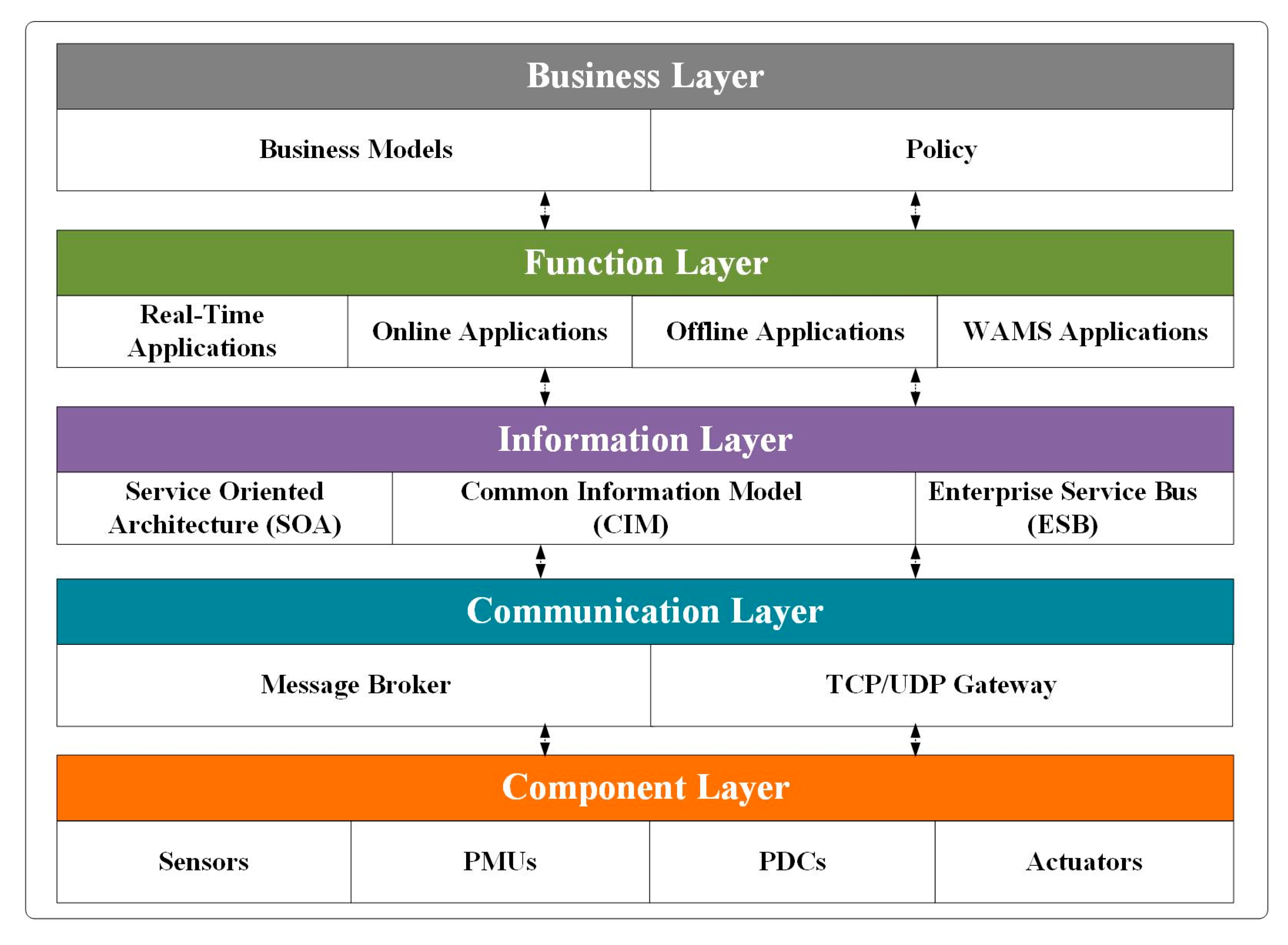
As shown in Figure 2, WAMS architecture includes five layers. The component layer consists of physical devices. It is responsible for providing data, functions, and communication services for the upper layers. The communication layer applies several methods and protocols to obtain data among various elements in the network. The information layer includes the data model and the communication rules that are used to exchange information. The function layer contains the logical functions or various WAMS applications, independent of the physical architecture; however, it is reliant on the business models and the organization’s policies. Finally, the business layer defines the business models and the policies [17,18]

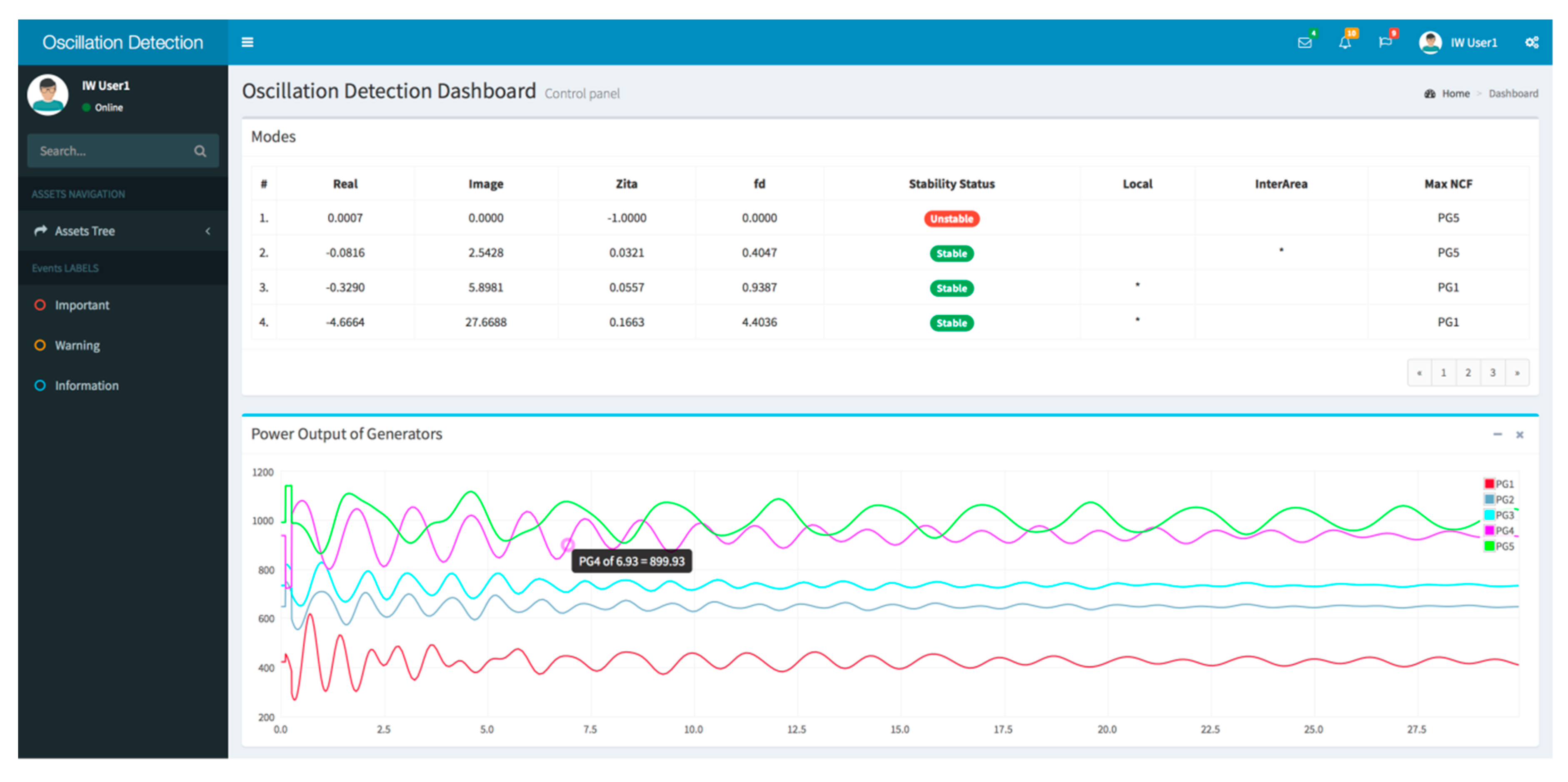
One of the main online applications associated with the proposed WAMS function layer is power system oscillation detection using synchrophasor data, which is the main scope of this paper. The oscillation detection algorithm is detailed in Section 2.2, Section 2.3, Section 2.4 and Section 2.5.

2.2. Motivation behind Methodology Selection

In many Smart Grid projects, some well-known methods used for power system oscillation detection were analyzed and compared. This has been carried out to identify the best method in terms of: (1) accuracy in the estimation of the oscillatory mode features, (2) simplicity in the implementation, (3) ability to provide visual intuitiveness, (4) skill to determine the most associated state variable to each oscillatory mode, (5) robustness against the noise, and (6) self-verification ability. A survey of the literature showed that the extended Prony methods can be a reasonable choice for the proposed framework. Note that the basic Prony method has some weakness such as its sensitivity to noise and selection of the proper order of the system [14,15,16]. An overestimated order may lead to the generation of extraneous modes by the Prony method. These drawbacks were addressed in some extensions of the Prony method. For example, the study in [15] proposed a simple criteria for selecting the order of the system. 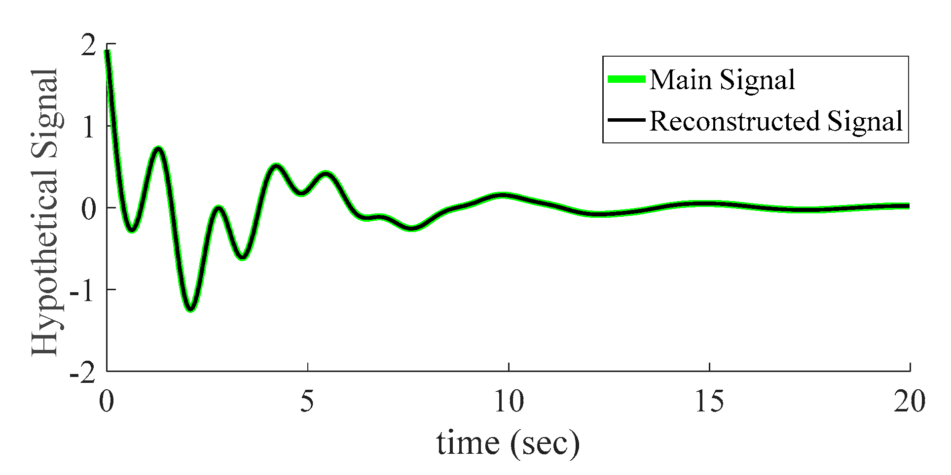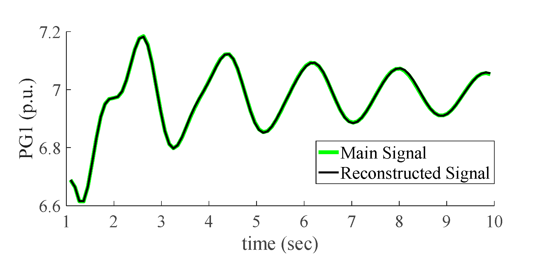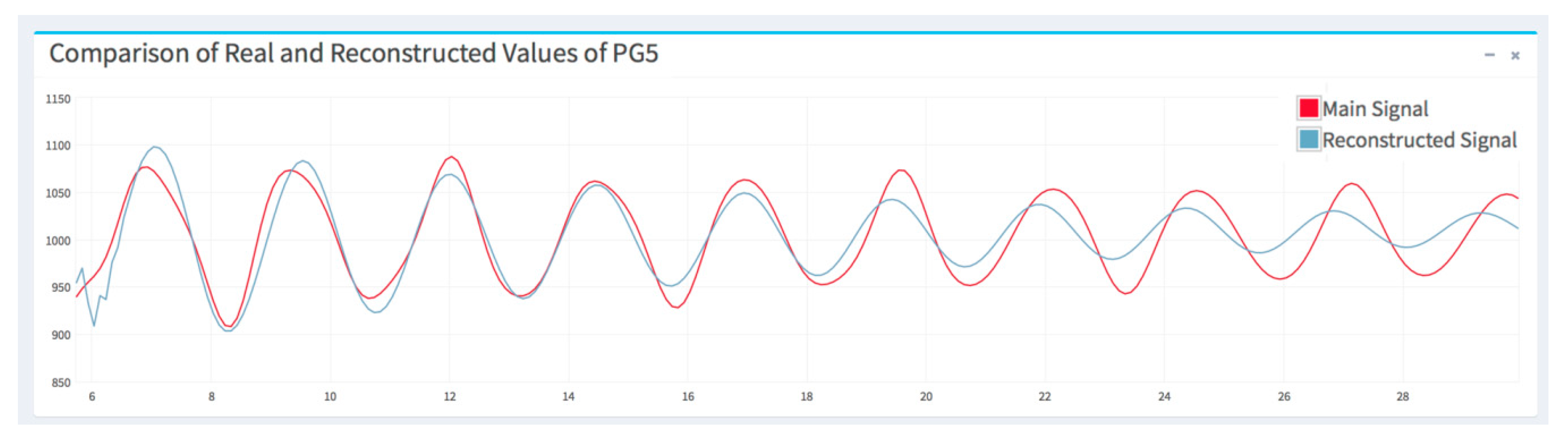The study in [16] suggested that the Prony method can be performed in forward and backward manners, where the final modes are selected from the collection of those extracted in such a process. This process enabled the Prony method to identify extraneous modes, while allowed elimination of the noise effects. Prony is inherently a self-verifiable method because it estimates the modes of a given signal and then reconstructs the main signal from the estimated mode. Comparing the main and the reconstructed signal is a convenient way to verify its performance.

The above features make the Prony method an effective one for practical applications; however, it does not provide visual intuitiveness on contribution various system modes in each oscillatory modes. This is important because power system operators are interested in visual information instead of numerical data. In this regard, the HHT method has advantages over the Prony method, in which the so-called IMFs plots represent the behavior of each mode intuitively, and therefore provide situational awareness on oscillations of the power system. Moreover, the HHT method can determine the contribution of a state variable in a mode based on energy and phase relationship of IMFs. Nevertheless, as stated in the introduction, the HHT method suffers from the EEs, mode-mixing and Gibbs phenomena [6,9]. In this paper, an improved Prony method is proposed that is able to calculate IMFs and thus NCFs for a given signal.

Note that HHT has a much wider application than the Prony method and the authors don’t mean the proposed method is generally better than HHT, especially in non-linear situations. We compare our method with HHT because it is the only method that can calculate IMFs and NCFs. To achieve the IMFs and NCFs, HHT should overcome some challenges such as end-effects, mode mixing, and Gibbs phenomena. These challenges are solved in different literature. 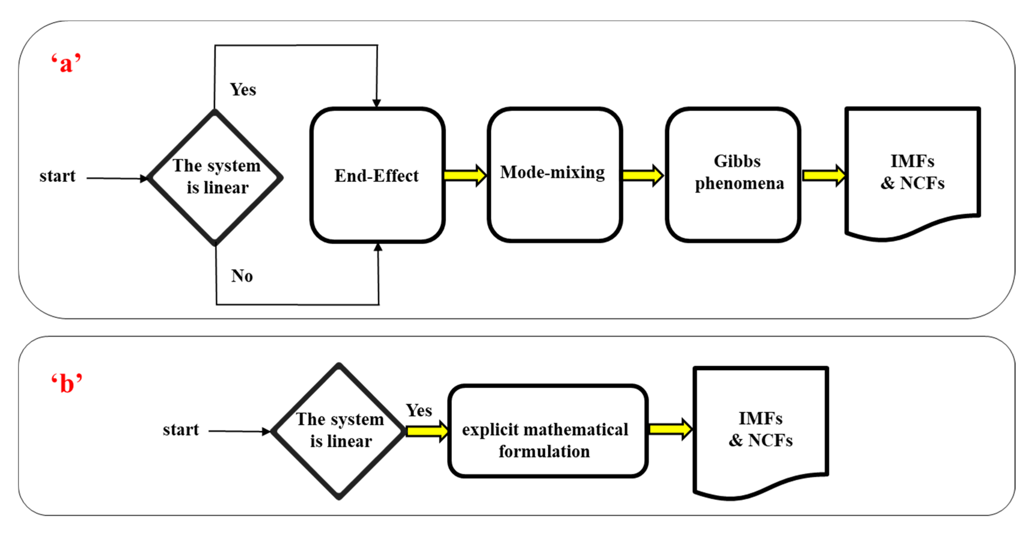For example, there are several ways to overcome end-effect issue [17]. In this paper, a direct method is proposed to obtain the IMFs and NCFs, in which the HHT challenges are avoided. Indeed, we are facing the alternative to obtain IMFs and NCFs as depicted in the following figure:

• HHT method that obtains IMFs and NCFs carefully, after solving the end-effects, mode mixing, and Gibbs phenomena. It is based on a heuristic, iterative method. Although it can handle non-linear situations [18], however, it is not the scope of this paper. Since we deal with the small signal stability assessment in which the linearization is an acceptable and reasonable assumption.
• Our Proposed method, which obtains IMFs and NCFs carefully, directly and without need to solve the end-effects, mode mixing, and Gibbs phenomena. It is based on an explicit mathematical formulation. It can be used for applications such as oscillation analysis, which is scope of this paper.

Therefore, both methods (HHT and proposed method) can handle the IMFs and NCFs with different approaches and can be used based on the situations. Figure 3, briefly shows the above discussions.

2.3. Oscillation Analysis Framework

Assuming a power system of order $n$, the zero-input time response is as follows [14]:

$$\underset{\_}{y}\left(t\right)={\displaystyle \sum }_{i=1}^n{\gamma }_i{e}^{{\lambda }_{i}t}$$

(1)

where ${\lambda }_i$ are called eigenvalues or modes of the system. The Prony method represents a given signal as a sum of exponential functions and then estimates the unknown parameters, i.e., ${\gamma }_i$ and ${\lambda }_i$ so that the real and the estimated output have a minimum difference. The estimated signal in the discrete time domain, and can be expressed as follows [14]:

$$\underset{\_}{\widehat{y}}\left(k\right)={\displaystyle \sum }_{i=1}^n{\beta }_i{z}_i{}^{k}k=1,2\dots ,N$$

(2)

where, $z_i$ are the eigenvalues of the system in the discrete time domain or z-domain,${\beta }_i$ is the residue corresponding to $z_i$ and $N$ is the number of the samples. Equation (2) can be described in a matrix form as [14]:

$$\left[\begin{array}{cccc}{z}_1{}^{1_s}& z_2{}^{1_s}& \cdots & z_n{}^1\\ z_1{}^{2_s}& z_2{}^{2_s}& \cdots & z_n{}^{2_s}\\ {⋮}_1{}^{N_s}& {⋮}_2{}^{N_s}& ⋮& {⋮}_N{}^{N_s}\\ z_1{}^N& z_2{}^N& \cdots & z_n{}^N\end{array}\right]\left[\begin{array}{c}{\beta }_1\\ {\beta }_2\\ ⋮\\ {\beta }_n\end{array}\right]=\left[\begin{array}{c}y(1)\\ y(2)\\ ⋮\\ y(N)\end{array}\right]$$

(3)

According to the Prony method, for a discrete time system with an output as (2), the so called characteristic equation is as follows [14]:

$$z^n-a_1{z}^{n-1}-a_2{z}^{n-2}-\cdots -a_{n-1}z-a_n=0$$

(4)

The coefficients of the above equation are obtained by solving the predictive equation as follows [14]:

$$\left[\begin{array}{ccc}y\left(n\right)& \cdots & y\left(1\right)\\ y\left(n+1\right)& \dots & y\left(2\right)\\ \begin{array}{c}⋮\\ y\left(N-1\right)\end{array}& \begin{array}{c}⋮\\ \dots \end{array}& \begin{array}{c}⋮\\ y\left(N-n\right)\end{array}\end{array}\right]\left[\begin{array}{c}{a}_1\\ a_2\\ \begin{array}{c}⋮\\ a_N\end{array}\end{array}\right]=\left[\begin{array}{c}y\left(n+1\right)\\ y\left(n+2\right)\\ \begin{array}{c}⋮\\ y\left(N\right)\end{array}\end{array}\right]$$

(5)

which can be given in a matrix form as:

$$D\underset{\_}{a}=\underset{\_}{d}$$

(6)

where, $D$ is the Prony Matrix. For WAMS-monitored power systems, both D and $\underset{\_}{d}$ contain synchrophasor data (e.g., voltages, currents, or powers). Based on the above formulations, the algorithm of the Prony method can be summarized as follows [14,15,16]:

• Constitute $D$ and $\underset{\_}{d}$ using PMU data according to (5).
• Solve a linear least square error (LSE) problem and obtain vector $\underset{\_}{a}$.
• Solve the polynomial characteristic Equation (4) to achieve the z-domain eigenvalues.
• Solve another LSE problem (3), using z values in Step 3.
• Reconstruct the main signal using (2).

Based on the above algorithm, in Step 3, the z-domain eigenvalues are calculated. The eigenvalues of the main signal can be obtained as follows [14]:

$$z_i=e^{{\lambda }_{i}T}\Rightarrow {\lambda }_i=\frac{log\left(z_i\right)}{T},i=1,2\dots ,n$$

(7)

where, $T$ is the sampling rate of the main signal. In many cases, instead of complex values of eigenvalues, two well-known parameters of the modes, i.e., damping ratio ξ and damping frequency $f_d$ are represented, which are related to eigenvalues as follows [1]:

$${\lambda }_i={\sigma }_i\pm j{\omega }_{d_i},{\xi }_i=\frac{{\sigma }_i}{\left|{\lambda }_i\right|},f_{d_i}=\frac{{\omega }_{d_i}}{2\pi },i=1,2\dots ,n$$

(8)

2.4. Calculation of IMFs and NCFs Based on Augmented Prony Method

As previously stated, an online oscillation monitoring framework should be able to determine the contribution of various system buses in each oscillatory mode. Here, as one of the novel contributions of this work, it is demonstrated that the Prony method can be used for such a purpose. Initially, the matrix $U$ is defined as follows:

$$U=\left[\begin{array}{cccc}{z}_1{}^{1_s}& z_2{}^{1_s}& \cdots & z_n{}^1\\ z_1{}^{2_s}& z_2{}^{2_s}& \cdots & z_n{}^{2_s}\\ {⋮}_1{}^{N_s}& {⋮}_2{}^{N_s}& ⋮& {⋮}_N{}^{N_s}\\ z_1{}^N& z_2{}^N& \cdots & z_n{}^N\end{array}\right]$$

(9)

where, $u_i$ is defined as column $i$ of matrix $U$, thus, for a complex eigenvalue, there is another eigenvalue which is the conjugate of $z_i$. Without the loss of generality, it is assumed that $z_{i+1}$ and ${\beta }_{i+1}$ are the conjugates of $z_i$ and ${\beta }_i$, respectively ($z_{i+1}=z_i{}^{*};{\beta }_{i+1}={\beta }_i{}^{*}$), thus:

$${\beta }_i{u}_i+{\beta }_{i+1}{u}_{i+1}={\beta }_i{u}_i+{\beta }_i{}^{*}{u}_i{}^{*},i=1,2\dots ,n$$

(10)

Substituting $u_i$ from (9) into (10) yields:

$${\beta }_i{u}_i+{\beta }_i{}^{*}{u}_i{}^{*}={\beta }_i\left[\begin{array}{c}{z}_i{}^1\\ z_i{}^2\\ ⋮\\ z_i{}^k\\ ⋮\\ z_i{}^N\end{array}\right]+{\beta }_i{}^{*}\left[\begin{array}{c}{\left(z_i{}^{*}\right)}^1\\ {\left(z_i{}^{*}\right)}^2\\ ⋮\\ {\left(z_i{}^{*}\right)}^k\\ ⋮\\ {\left(z_i{}^{*}\right)}^N\end{array}\right],i=1,2\dots ,n$$

(11)

where, ${\beta }_i$ and $z_i$ are defined as follows:

$$z_i=e^{{\lambda }_{i}T}=e^{\left({\sigma }_i+j{\omega }_d{}_i\right)T},{\beta }_i=\frac{A_i}{2}{e}^{j{\phi }_i},i=1,2\dots ,n$$

(12)

Thus, (11) can be rewritten as:

$${\beta }_i{\mu }_i+{\beta }_i{}^{*}{\mu }_i{}^{*}=\left[\begin{array}{c}{A}_i{e}^{{\delta }_{i}T}cos[{\omega }_{d_i}T+{\phi }_i]\\ A_i{e}^{{\delta }_i(2T)}cos[{\omega }_{d_i}(2T)+{\phi }_i]\\ ⋮\\ A_i{e}^{{\delta }_i(kT)}cos[{\omega }_{d_i}(kT)+{\phi }_i]\\ ⋮\\ A_i{e}^{{\delta }_i(NT)}cos[{\omega }_{d_i}(NT)+{\phi }_i]\end{array}\right],i=1,2\dots ,n$$

(13)

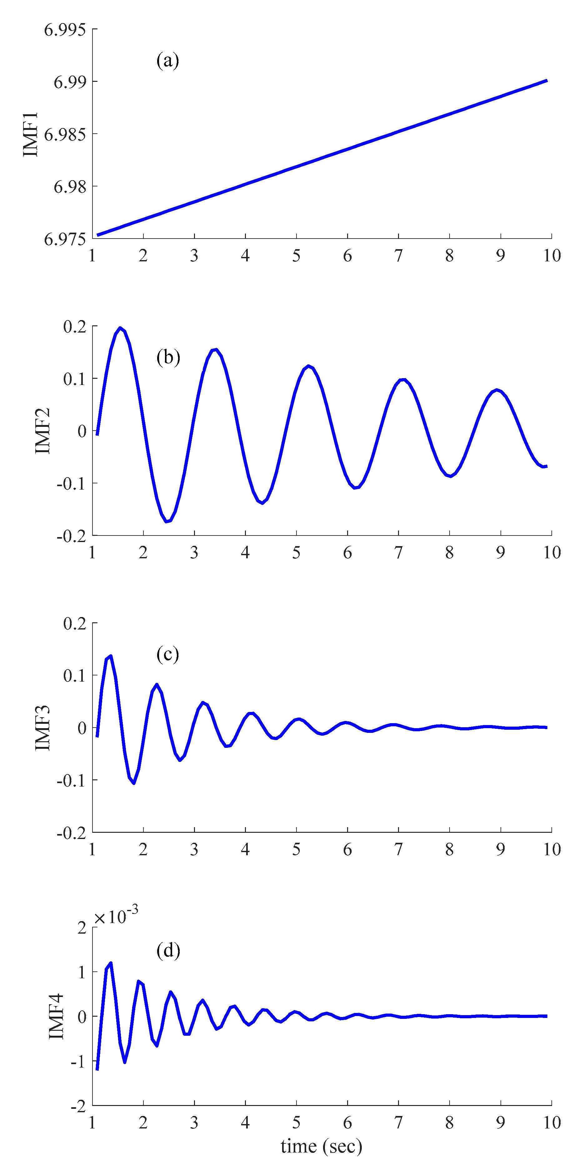
According to the definition of IMF (each of the exponential sinusoids contained in the main signal), the kth row of the vector in (13) shows the value of IMF of mode $i$ at the time $t=kT$. Thus, IMFs can be calculated as in (14):

$$IM{F}_i\left(t=kT\right)={\beta }_i{u}_i\left(k\right)+{\beta }_i{}^{*}{u}_i{}^{*}\left(k\right),i=1,2\dots ,n$$

(14)

The above expression is valid for complex modes. For any real mode, its corresponding column in matrix $U$ results in values of $IM{F}_i$. Therefore, a generalized form for the calculation of IMFs can be expressed as:

$$IM{F}_i\left(t=kT\right)={\beta }_i{u}_i\left(k\right)+c_i{\beta }_i{}^{*}{u}_i{}^{*}\left(k\right),i=1,2\dots ,n$$

(15)

where, $c_i$ is a binary variable that shows either mode $i$ is complex ($c_i=1$) or not ($c_i=0$). Note that it is assumed in (15) that columns of the matrix $U$ are sorted based on their real part.

Having intrinsic function of each mode, it is possible to determine the most associated state variable corresponding to each oscillatory mode, using energy and phase relationship of IMFs. In other words, the generator or actuator that is the most associated ones with a specific mode can be identified. As mentioned in the Introduction, the participation of each system bus in an oscillatory mode can be determined using node contribution factor (NCF). This index is defined as follows:

$$NC{F}_{s,i}=E_{s,i}cos({\phi }_{s,i})$$

(16)

where, $NC{F}_{s.i}$ represents the contribution of signal $s$ in mode $i$. $E_{s,i}$ is defined as the energy of ${\mathrm{IMF}}_{\mathrm{i}}$ (related to mode $i$) obtained by signal $s$, which is defined as follows:

$$E_{s,i}={\displaystyle \sum }_{k=1}^{N}IM{F}_{s,i}{}^2\left(t=kT\right)$$

(17)

In (16), ${\phi }_{s,i}$ is the average relative phase of $IM{F}_{s,i}$ and the first IMF ($IM{F}_{s,1}$ that is associated with the dominant mode) in different times:

$${\phi }_{s,i}=\left(\frac{1}{N}\right).{\displaystyle \sum }_{t=1}^N{\theta }_{s,i}\left(t\right)-{\theta }_{s,1}\left(t\right)$$

(18)

In order to calculate ${\phi }_{s,i}$ a phase angle is assigned to each data point of $IM{F}_{s,i}$. For all IMFs extracted from a measured signal of the network, the initial phase angle of the first IMF is defined as the reference phase (${\theta }_{s,1}\left(t\right)=0$). For a specific IMF, the phase angle of maximum, minimum, positive zero-crossing, and the negative zero-crossing points are set as π/2, 3π/2, 0 (or 2π) and π, respectively. According to the proposed formulation in (15)–(18), it is possible to directly calculate IMFs of the various signals of the system and therefore obtain their contributions in the different oscillatory modes. It is important to emphasize that so far, the Prony method has not been augmented for calculation of IMFs and thus NCFs. Our proposed formulation in this subsection bypasses the problems of nonlinear and the iterative method of HHT method for IMF calculation, such as the mode mixing of EMD, end effect and Gibbs phenomena [6,7,8,9].

Note that the understudy signal may contain noise that can be easily eliminated before performing the proposed method. It is worth mentioning that the mode mixing phenomena is not related to the noise. In the HHT method the IMFs are obtained using an iterative procedure with two loops, the outer loop repeats with the number of modes and for each mode an iterative procedure called sifting is performed to achieve the IMF associated with that mode. When the frequency of two modes of the system is close to each other, mode mixing may have occurred. In fact it is related to frequency heterodyne. Therefore, noise that is a high frequency signal may not mix with power system modes, which are low-frequency modes. In our proposed method, all sifting or decomposition procedures are not performed; therefore it is not prone to mode mixing. In the proposed method, each mode has a unique IMF. Thus, with an explicit mathematical formulation, each mode and its IMF are specifically extracted.

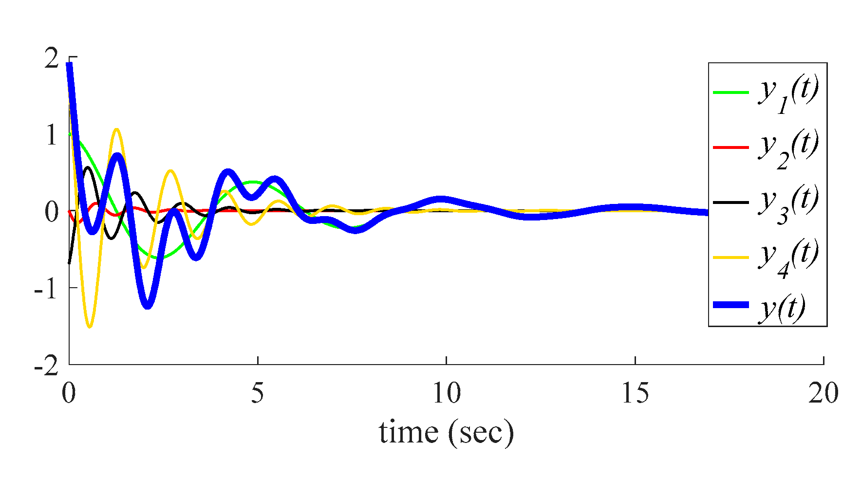
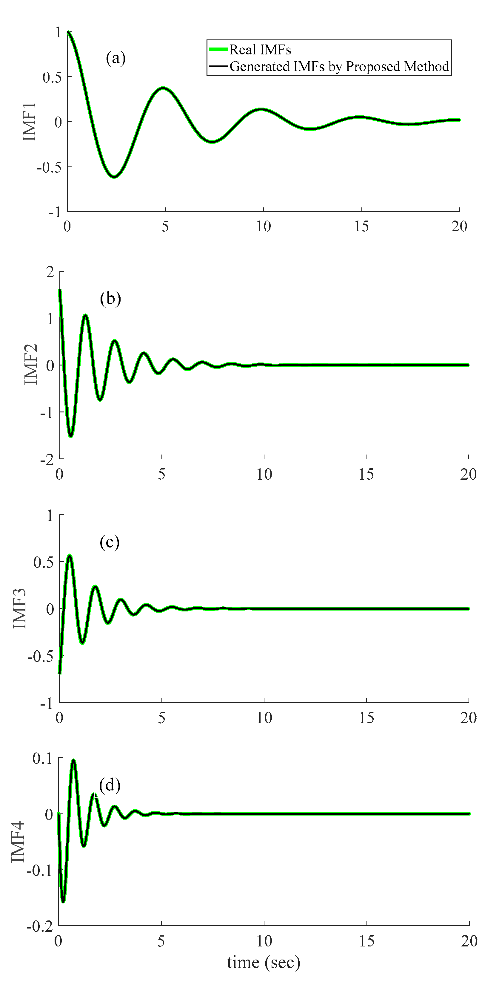
It is worth mentioning that power system oscillation detection and analysis is one of the topics of small signal stability assessment. In small signal stability assessment and analysis, it is generally accepted that the variation of the state variables of the system around the operating point are small, thus the differential equations of the system can reasonably be linearized at the operating point. The zero-input time response of such equations is seen in Equation (1). Therefore, despite the HHT method can handle signals without assumption of structure in Equation (1), in small signal stability analysis, which is the scope of this paper, we deal with the exponential sinusoids signals called intrinsic mode functions (IMFs). It is worth mentioning that the method is performed on many different signals with different parameters (amplitude, damping, frequency, and phase angle), and in all cases, the performance of the method in estimation of the mode parameters and extraction of the IMFs, are approved. However, an example of such signal is presented in Section 3.1.

2.5. Approximation System Order

In practical situations, the number of modes incorporated in the signal is unknown. Several methods are proposed in the literature to approximate the effective order of the system [14,15,16]. In this paper, a new IMF-based index is introduced to determine the effective system order. The smallest index m that satisfies the inequality in (18) is the effective order of the system.

$$\frac{{{\displaystyle \sum }}_{i=1}^{m}IM{F}_{s,i}{}^2}{{{\displaystyle \sum }}_{i=1}^{n}IM{F}_{s,i}{}^2}\ge \tau$$

(19)

where, the threshold value $\tau$ is close to 1 (e.g., 0.999) and $n$ is the initial value of the system order.

3. Simulation Results and Discussion

3.1. Test Case 1: Hypothetical Signal

In this test case, a hypothetical signal give in (20) with four pairs of complex conjugate eigenvalues is considered. Parameters of this signal are shown in

Table 1. Parameters of the Hypothetical Signal of Test Case 1.

$\mathit{j}$	${\mathit{A}}_{\mathit{j}}$	${\mathit{\sigma }}_{\mathit{j}}$	${\mathit{f}}_{\mathit{d}}{}_{\mathit{j}}$	${\mathit{\phi }}_{\mathit{j}}$
1	1	−0.2	0.2	0
2	0.2	−1	1	$\mathsf{\pi }/2$
3	−0.8	−0.7	0.8	$\mathsf{\pi }/6$
4	2	−0.5	0.7	$\mathsf{\pi }/5$

. The main signal (i.e., $y\left(t\right)$) and its components (i.e., $y_1\left(t\right)\mathrm{to}{y}_4\left(t\right)$) are shown in Figure 4. It is assumed that signal $y\left(t\right)$ is measured by PMU and resampled at 10 Hz used as an input of our proposed method. The main advantage of this test case is that the real modes and their corresponding IMFs are predefined, thus it is suitable for the validation of the proposed method. The jth mode associated with $y\left(t\right)$ can be calculated according to (8). Also, $y_j\left(t\right)$ is by definition the jth IMF. The main signal is compared with the reconstructed signal by the Prony method in Figure 4. As shown in Figure 5, the reconstructed signal completely matches the real signal $y\left(t\right)$, as expected. As stated in Section 2.3, Figure 5 illustrates the self-verification property of the Prony method.

$$y\left(t\right)={\displaystyle \sum }_{j=1}^4{y}_j\left(t\right)={\displaystyle \sum }_{j=1}^4{A}_j{e}^{{\sigma }_{j}T}cos\left[2\pi f_d{}_{j}t+{\phi }_j\right]$$

(20)

The modes of the signal $y\left(t\right)$ obtained by the Prony method are compared with real modes in

Table 2. Calculated Modes of Test Case 1.

Real Modes		Estimated Modes
$\mathit{\xi }(-)$	${\mathit{f}}_{\mathit{d}}\left(\mathit{H}\mathit{z}\right)$	$\mathit{\xi }(-)$	${\mathit{f}}_{\mathit{d}}\left(\mathit{H}\mathit{z}\right)$
0.157	0.2	0.157	0.2
0.113	0.7	0.113	0.7
0.138	0.8	0.138	0.8
0.157	1	0.157	1

. Observe that the Prony method is capable to extract modes accurately. The IMFs of the hypothetical signal are shown in Figure 6. Observe that extracted IMFs from our proposed mathematical method in Section 2.4 are exactly the same as real IMFs ($y_j\left(t\right);j=1,\dots ,4)$. Thus, our mathematical formulation computes IMFs of a given signal with high accuracy, without a need for heuristic algorithms such as those employed in the HHT method. Also, as illustrated in Figure 6, the proposed method represents IMFs of a given signal, in order of increasing damping for them. In other words, IMF of a more dominant mode or equivalently less damped ones will be represented first in our methodology. Therefore, in the Test Case 1, ${\mathrm{IMF}}_1$ to ${\mathrm{IMF}}_4$ are corresponding to $y_1$, $y_4$, $y_3$, and $y_2$ in the hypothetical signal of (20), respectively, shown in Figure 4.

3.2. Test Case 2: Kundur’s Two-Area Power System

The second test case is carried out using Kundur’s two-area test system [1], which is shown in Figure 7. These two areas are connected through weak transmission lines. The output active power of the generators denoted after the occurrence of a three-phase short-circuit fault is shown in Figure 8. The fault occurred at t = 1 s on Bus 8 and was cleared at t = 1.05 s. Assume that PG1 to PG4 are the output active power of the generators G1 to G4, respectively. Each of the four signals is analyzing using the proposed method in Section 2.3 and Section 2.4 to extract modes of the system, their IMFs and consequently NCFs. The extracted modes based on each signal are depicted in

Table 3. Comparison of Extracted Modes based on Active Power of Different Generators in Test Case 2; $\xi (-),f_d\left(Hz\right)$.

G1		G2		G3		G4
$\mathit{\xi }$	${\mathit{f}}_{\mathit{d}}$	$\mathit{\xi }$	${\mathit{f}}_{\mathit{d}}$	$\mathit{\xi }$	${\mathit{f}}_{\mathit{d}}$	$\mathit{\xi }$	${\mathit{f}}_{\mathit{d}}$
–1	0	–1	0	–1	0	–1	0
1	0	1	0	1	0	1	0
0.037	0.49	0.034	0.49	0.033	0.49	0.043	0.49
0.085	0.97	0.081	0.95	0.088	0.94	0.083	0.98

. It is evident from the table that the extracted modes from the different signal (i.e., PG1 to PG4) result in the same modes. This is one way to validate the accuracy of the modes obtained by the Prony method. The main and reconstructed values of PG1 by the proposed method are compared in Figure 9, where again the accuracy of our framework is demonstrated. The extracted IMFs from generator G1 output power are demonstrated in Figure 10. Observe that ${\mathrm{IMF}}_1$ is associated with an unstable mode, while the other three modes are under-damped. While analyzing numerical results of Table 3 is important, our framework provides visual information using IMF plots (using the proposed formulation in Section 2.4) such as the one shown in Figure 10, which provides situational awareness for oscillations during the fault.

Finally, based on energy and phase angle of IMFs, contribution factor of each generator output power in each of the modes can be determined, as demonstrated in

Table 4. Node contribution factor (NCF) matrix in Case 2.

Signal\Mode	Mode 1	Mode 2	Mode 3	Mod 4
PG1	4827.053	0.855	0.123	0.000
PG2	4825.077	0.120	0.059	0.000
PG3	4825.284	0.219	0.032	0.000
PG4	5090.697	1.031	0.000	0.072

.

The matrix in Table 4 implies that the most associated generation in oscillatory modes 1, 2, and 4 is generator G4, while mode 3 is mainly affected by generator G1.

3.3. Test Case 3: Interconnected Practical Power System

In this section, the proposed method of Section 2.3, Section 2.4 and Section 2.5 has been used to analyze measured signals in a practical transmission power system. The output powers of the five generators resampled at 10 Hz are used to demonstrate performance of the proposed method. All presented results in this section are generated by the interconnected power system WAMS-based oscillation detection application utilizing our proposed method of Section 2.3, Section 2.4 and Section 2.5. A general schematic of this application is demonstrated in Figure 11. The signals related to five generators (here they are named G1 to G5) associated with the area that are affected by the fault are depicted in Figure 11. As shown in Figure 11, the information of oscillatory modes are provided to the system operator in a format of a table. Columns 1 to 4 in the table represent real and imaginary part of each oscillator mode, and their damping ratio and frequency, respectively. Moreover, the fifth column demonstrates stability status of each mode. For example, as shown in Figure 11, the first mode is an unstable mode shown with red color. The next columns show type of modes based on their frequency, i.e., local or inter-area. According to Figure 11, mode 2 is an inter-area mode with frequency of 0.4 Hz, while Modes 3 and 4 are local modes with frequency of 0.94 and 4.4 Hz due to oscillation of Generator G1 output power.

As an example, the comparison of the original and reconstructed generation G5 signal based on the Prony-based method is shown in Figure 12, which demonstrates an acceptable matching between two signals. The accuracy of the modes and consequently IMFs and NCFs can be concluded from this matching. Having IMFs associated with all five generation signals, a NCF matrix with five rows and four columns is calculated by our framework (see Section 2.4), as shown in

Table 5. NCF Matrix in Test Case 3.

Signal\Mode	Mode 1	Mode 2	Mode 3	Mode 4
PG1	0.437 $\times$ 108	1.349 $\times$ 105	4.662 $\times$ 104	2.28 $\times$ 103
PG2	1.023 $\times$ 108	0.138 $\times$ 105	507	399
PG3	1.314 $\times$ 108	0.163 $\times$ 105	140	497
PG4	2.140 $\times$ 108	1.764 $\times$ 105	136	2.85 $\times$ 103
PG5	2.448 $\times$ 108	4.631 $\times$ 105	1.380 $\times$ 104	3.91 $\times$ 103

. This table shows that, the most associated signal to modes 1, 2, and 4 is G5 and mode 3 is mainly affected by G1. Thus, for controlling and stabilizing the system against the unstable mode (mode 1), also increasing the damping of the poorly damped mode 4, G5 should be controlled. Also, observe that generation G3 is the most suitable actuator for controlling mode 3. As seen from Table 5, the energy of the mode 2 is less than mode 1, while the energy of modes 3 and 4 relative to mode 2 is insignificant. Note that as the energy of the other modes is negligible, our oscillation detection framework discards them from the representation of their parameters as well as IMFs and NCFs. For better representing the contribution of each generator in each mode, the values of the NCF matrix are normalized and plotted in Figure 13. Other important plots in the power system oscillation detection application are related to IMFs of the measured signals, which are not shown here for brevity. The plot is similar to those shown in Figure 6 and Figure 10 in Test Case 1 and 2, respectively. These provide an increase intuitiveness in the proposed oscillation detection framework, beside NCF plots. It was observed in IMF plots that the main or dominant mode (mode 1) has a growing IMF as it is unstable, while the other modes (mode 2 to 5) have exponential sinusoidal IMFs which are damped after 40, 20, and 7 s, respectively.

3.4. Comparison with Related Methods

In this section, we show the superiority of the proposed method for oscillation analysis. Due to space limitations, the proposed augmented Prony-based oscillation analysis is compared with the well-known and adopted techniques such as HHT and conventional Prony methods. It is clear from

Table 6. Comparison of the Proposed and Other Related Works.

Method\Index	IMF	NCF	Computational. Complexity	EE	Gibbs	Mode-mixing
HHT	$\surd$	$\surd$	O (nm)	$\times$	$\times$	$\times$
Conventional Prony	$\times$	$\times$	-	-	-	-
Proposed method	$\surd$	$\surd$	O (1)	$\surd$	$\surd$	$\surd$

that the proposed method is superior to others in terms of indices such as IMF, NCF, computational complexity, EE, Gibbs, and mode-mixing. For instance, the proposed method can eliminate the worse effects of EE, Gibbs and mode-mixing where other methods cannot. Considering the computation burden as an index, the proposed method is superior to HHT in which the complexity order of the proposed augmented method and HHT are O (1) and O ($\mathrm{n}\times \mathrm{m}$), respectively. Where $\mathrm{n}$ is the number of the desired modes and $\mathrm{m}$ is the number of iterations in EMD process.

In order to further verify the proposed method, the results of the Test case 2 is compared with the results of PSAT software which is a MATLAB-based software, which can be used for small-signal stability analysis. Note that the analysis of PSAT is based on the detailed modeling of the generators, automatic voltage regulators (AVRs), power system stabilizers, PSSs, etc., whereas the proposed method is based on the synchrophasor measurements and the modeling of power system components is not needed. As seen from

Table 7. The Results of Test Case 2, Obtained by Detailed Modeling of Power System in PSAT Software.

Eigevalue	Most Associated States		Real Part	Imag. Part	Damping Ratio	freq
Eig #1	e2q_Syn_2		−36.498	0.000	1.000	0.000
Eig #2	e2q_Syn_4		−36.423	0.000	1.000	0.000
Eig #3	e2q_Syn_3		−34.055	0.000	1.000	0.000
Eig #4	e2q_Syn_1		−32.733	0.000	1.000	0.000
Eig #5	e2d_Syn_1		−30.466	0.000	1.000	0.000
Eig #6	e2d_Syn_2		−30.257	0.000	1.000	0.000
Eig #7	e2d_Syn_4		−23.408	0.000	1.000	0.000
Eig #8	e2d_Syn_3		−21.699	0.000	1.000	0.000
Eig #9	delta_Syn_1,	omega_Syn_1	−0.562	6.798	0.082	1.082
Eig #10	delta_Syn_1,	omega_Syn_1	−0.562	−6.798	0.082	1.082
Eig #11	omega_Syn_2,	delta_Syn_2	−0.561	6.610	0.085	1.052
Eig #12	omega_Syn_2,	delta_Syn_2	−0.561	−6.610	0.085	1.052
Eig #13	delta_Syn_4,	omega_Syn_4	−0.126	3.457	0.036	0.550
Eig #14	delta_Syn_4,	omega_Syn_4	−0.126	−3.457	0.036	0.550
Eig #15	e1d_Syn_1		−5.835	0.000	1.000	0.000
Eig #16	e1d_Syn_2		−5.787	0.000	1.000	0.000
Eig #17	e1d_Syn_4		−4.388	0.000	1.000	0.000
Eig #18	e1d_Syn_3		−3.495	0.000	1.000	0.000
Eig #19	e1q_Syn_1		−0.171	0.000	1.000	0.000
Eig #20	e1q_Syn_2		−0.179	0.000	1.000	0.000
Eig #21	omega_Syn_4		−0.069	0.000	1.000	0.000
Eig #22	delta_Syn_4		0.010	0.000	−1.000	0.000
Eig #23	delta_Syn_4		0.000	0.000	NaN	0.000
Eig#24	omega_Syn_4		0.000	0.000	NaN	0.000

, the damping ratio and frequency of the dominant modes (Eig #21, Eig #22, Eig #13, and Eig #14) of the studied power system obtained by the detailed modeling in PSAT are comparable with the results of proposed method presented in Table 3. Both results, demonstrates that the dominant mode is an unstable mode. One of the capabilities of the PSAT toolbox is that it can determine the most-associated states related to each mode. The PSAT determines this using participation factors (PP) which be calculated using the elements of the state matrix A (if we consider the state equations as $\dot{\mathrm{x}}=\mathrm{Ax}+\mathrm{Bu}$). Alternatively, in this paper we determine the most associated state variable corresponding to each oscillatory mode using the NCF index without the need to detail modeling of the system. As can be seen from Table 7, based on the PSAT results, the most associated generation in oscillatory modes 1, 2 is generator G4 which complies with the results obtained based on the NCF index in the proposed method.

4. Conclusions

In this paper, an online WAMS-based power system oscillation analysis framework was proposed. Features of the Prony method, such as simplicity in the implementation, self-verification, and robustness against the noise to estimate the modal information of a measured signal (i.e., its damping and frequency), nominated it for practical applications. The Prony method is then augmented here to be able to calculate IMFs and thus NCFs. IMFs provide an intuitive representation of the system modes and are mainly calculated using the iterative HHT-based methods. Our proposed framework calculates IMFs using an explicit mathematical formulation based on the augmented Prony method directly from PMU measurements. Therefore, it is simpler, faster and more accurate compared to those methodologies. The proposed Prony-based NCF index of this paper allowsthe identification of the most associated state variable to each mode accurately.

The simulation results on three test cases revealed that the proposed framework is able to determine IMFs and NCFs more accurately.