An Influencing Parameters Analysis of District Heating Network Time Delays Based on the CFD Method


School of Environmental Science and Engineering, Tianjin University, Tianjin 300072, China
*
Author to whom correspondence should be addressed.
Energies 2019, 12(7), 1297; https://0-doi-org.brum.beds.ac.uk/10.3390/en12071297
Submission received: 11 March 2019
/
Revised: 28 March 2019
/
Accepted: 2 April 2019
/
Published: 4 April 2019
(This article belongs to the Special Issue District Heating and Cooling Networks)
Abstract
:With the expansion of cities, district heating (DH) networks are playing an increasingly important role. The energy consumption due to the time delay caused by the transport of the medium in the DH network is enormous, especially in large networks. The study of time delay is necessary for the operation and optimization of DH networks. Compared with previous studies of constant flow rates and ideal pipeline (without regard to branches, elbows, variable pipe diameters, etc), this paper simulates a DH network in Tianjin University, China, by establishing the actual engineering model in a Computational Fluid Dynamics (CFD) method to analyze the time delay. The CFD model has great advantages in terms of computational cost and application range compared to theoretical calculations. The peak-valley method was used to verify the correctness of the time delay simulation model. Results show that the time delay calculated by the CFD model is consistent with the actual time delay obtained from the measured data. Based on this model, the parameters that affect the time delay are furtherly analyzed. Four key parameters, including flow rate, pipe length, pipe diameter, and water supply temperature are summarized. The results show that the flow rate, pipe length and pipe diameter have a great influence on the time delay of the DH network, while the temperature has little effect on the time delay. The time delay of the DH network system has a significant impact and can provide services for optimal control of the system.
1. Introduction
DH (District heating) networks are considered a very efficient option for providing heating and domestic hot water to buildings, particularly for densely populated areas [1]. DH systems are community energy systems which can provide long-term achievements in terms of greenhouse gas emission abatement, energy security, local economic development, energy, and exergy efficiencies increase and exploitation of renewable energy [2]. Improving the heating performance of DH networks, one of the most important components in district heating systems, has a significant influence on the promotion of energy efficiency [3].
The behavior and characteristics of the DH network system are influenced by its various parameters [4]. The dynamic features of DH consumers and networks usually influence the operational effect of the DH system heavily because of the time delays in the DH system [5]. It may take a huge amount of time for the further located ends to response to heat injection. The time delay of heat transportation can reach minutes or hours [6]. The existence of time delays usually results in a mismatch between the heat source output and the users’ heating load [7], and considerable heat loss [8]. The optimization of system control [9,10] to reduce the energy losses caused by time delays has attracted more and more scholars’ attention.
In the published papers, many researchers focus on the dynamic characteristics of heating networks. A method for calculating the time delay of the network was presented by Jie, et al [11] who using physical and mathematical models, proved that in the case of a single straight pipe with constant pipe diameter, the time delay was approximately equal to the flow time of the heat medium. Zheng [12] proposed a new physical method (function method) and corresponding dynamic temperature simulation computer code to analyze the thermal dynamic characteristics of the district heating network, focusing on the dynamic temperature distribution. The results showed that the function method could be recommended to simulate the dynamic temperature of district heating network accurately and quickly for efficient system performance. Wang and Meng [13] used the third-order numerical solution method to investigate the influence of thermal inertia of the pipe wall on the thermal transient prediction model of a long pipe. The results show that for pipes with a diameter greater than 200, it is not necessary to consider the influence of thermal inertia in the modeling process.
Some scholars also focused on research on control strategies in terms of time delay. Li [14] proposed a special control strategy called Smith predictor which took the transport time delay out of the closed-loop feedback control system to deal with the effects of transport delay problem. Sartor [15] proposed a dynamic model of the heat wave in the network to determine the temperature and mass flow in some key locations to solve the problem of excessive delay time in the DH network. Additionally, some authors focus on the dynamic simulations of DH systems. In [16,17], the validation of the simplified approaches based on practical comprehensive DH systems was formulated, but the case was validated for a single pipe or several branches, the validations performing on a full system are limited. Gabrielaitiene [18] modeled a DH system in Denmark by a node method and TERMIS software and indicated that the local discrepancies between the predicted and measured supply temperatures were pronounced for consumers located at distant pipelines containing numerous bends and other fittings. Mattias [19] used a simulation tool developed in MATLAB/Simulink to analyze the flow distribution in the district heating network behavior, the results showed that the tool was a valuable instrument to simulate and analyze the behavior of meshed district heating network.
It can be seen that the function method is mainly based on the mathematical model and the construction of the physical model to calculate the time delay and temperature distribution of the DH network system. However, the proposed function method is only suitable for the single-pipe solution, which is limited by the computational cost and the complexity of the pipe network for large DH networks. Therefore, the calculation of the time delay of the DH network system caused by temperature change is inaccurate. The method of simulation such as MATLAB/Simulink, which also can prove that the mathematical method used to determine the temperature distribution of the elbow and other fittings of the long pipe is unreasonable, has a potential for simulating the temperature distribution in the DH network system and calculating the time delay caused by the flow. However, the establishment of the Simulink module of each node requires the basis of the mathematical model and the flow state parameters. Some simulation research on the optimal control of the DH network system to reduce the impact of time delay on system control, ignoring the main factors causing the time delay of the DH network system. This paper focused on the calculation method of the time delay of the DH network system, which was determined by establishing a CFD model. The combination of steady-state calculation and transient calculation solves the established DH network model. Compared with the calculation method of time delay theory in the previous articles, the relative degree of CFD method reduces the calculation cost and breaks through the constraints of the pipeline model, which is not only limited to a single pipe, but the time delay of the fluid through the varying diameters, bends, and branches can also be calculated. Compared with some other simulation methods, only simple boundary conditions need to be obtained without the operation parameters inside the pipe of the DH network system. The DH network of Tianjin University was taken as the research object. The time delay of the DH network obtained by using the CFD model was compared with the measured data to verify the correctness of the model. The results show that the proposed CFD model is superior in calculating the time delay of the DH network. Based on the CFD model, the parameters affecting the time delay were analyzed. The time delay of the DH network system obtained by the CFD simulation method can be used as a reference for the optimization of a DH network system to ensure that the operating parameters of the DH network and the heat load requirements of the heat consumers can be matched in time.
2. DH Network System Description
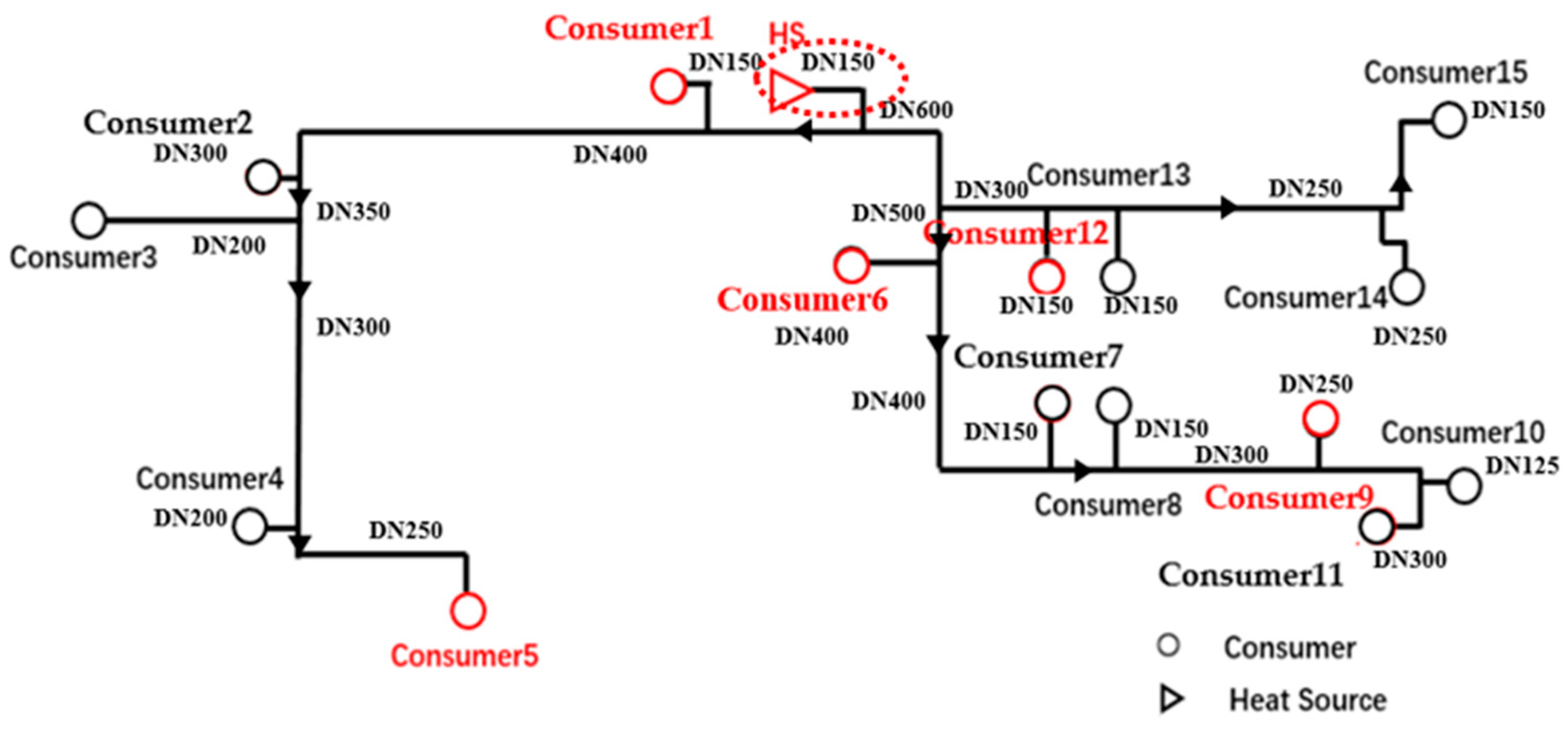
The studied system is located at Tianjin University. The heat source is composed of a ground-source heat pump and boiler, which serves more than 265600 square meters of building area. The DH network system supplies heat to 15 consumers, which includes a library, teaching building, laboratories and so on. Figure 1 shows the distribution network of the Tianjin University subsystem. In this case, there is no substation and the consumer is a terminal building. The heat source directly transfers the heat through the DH network to the terminal building. The network is constructed of pre-insulated pipes with a total length of approximately 1.8 km. The pipe diameter ranges from 125 mm to 600 mm. The distance between the heat consumer and the heat source is shown in Table 1. The closest and farthest to the heat source are the heat consumer 1 and the heat consumer 5, which are 145 m and 633 m, respectively.
Considering the similarities of the building functions and the symmetry of the actual distribution of the pipe network, five typical consumers were selected for test verification. The functions of each consumer and the distance from the heat source are shown in Table 1.
3. Methodology
3.1. Computational Fluid Dynamics Modelling
3.1.1. CFD Model and Preliminary Settings
Since numerical simulation has unique advantages over experimental studies, such as low cost and short cycle time, complete data can be obtained and various measured data states can be simulated during actual operation [20]. Fluent is a commercial software package that uses a finite volume method to couple mass equations, momentum equations, and energy equations. The flow in the pipe is an incompressible fluid that satisfies the general governing equation describing the state of the flow field as a flow pattern. The basic governing equations are shown in Equations (1)–(3). A coupled solution based on three equations of a powerful workstation can be solved. In this study, Fluent 17.0 was used for our numerical simulation calculations. The workstation for the simulation calculation is an Asus Z10PA-D8 2.20 GHz, 64GB of RAM and 120 GB of hard drive memory. The CPU of this workstation is an Inter(R) Xeon(R) CPU E5-2630 v4 @ 2.20 GHz. A parallel computing technique was implemented in ANSYS Fluent solver:
where is the density, t the time, v the velocity, p the pressure, the shear stress, g the gravity acceleration, cv and cp the specific heats, T the temperature and kT the thermal conductivity.
The workflow of the model is mainly composed of the following aspects:
- The STEP AP214 format in SOLIDWORKS was used to generate simplified 2D CAD
- A structured mesh based on ICEM was generated. The maximum mesh size was defined as 30. The minimum orthogonal quality of the mesh is 0.932 and the maximum orthogonal skewness is 0.068
3.1.2. Setting the Fluent Solver
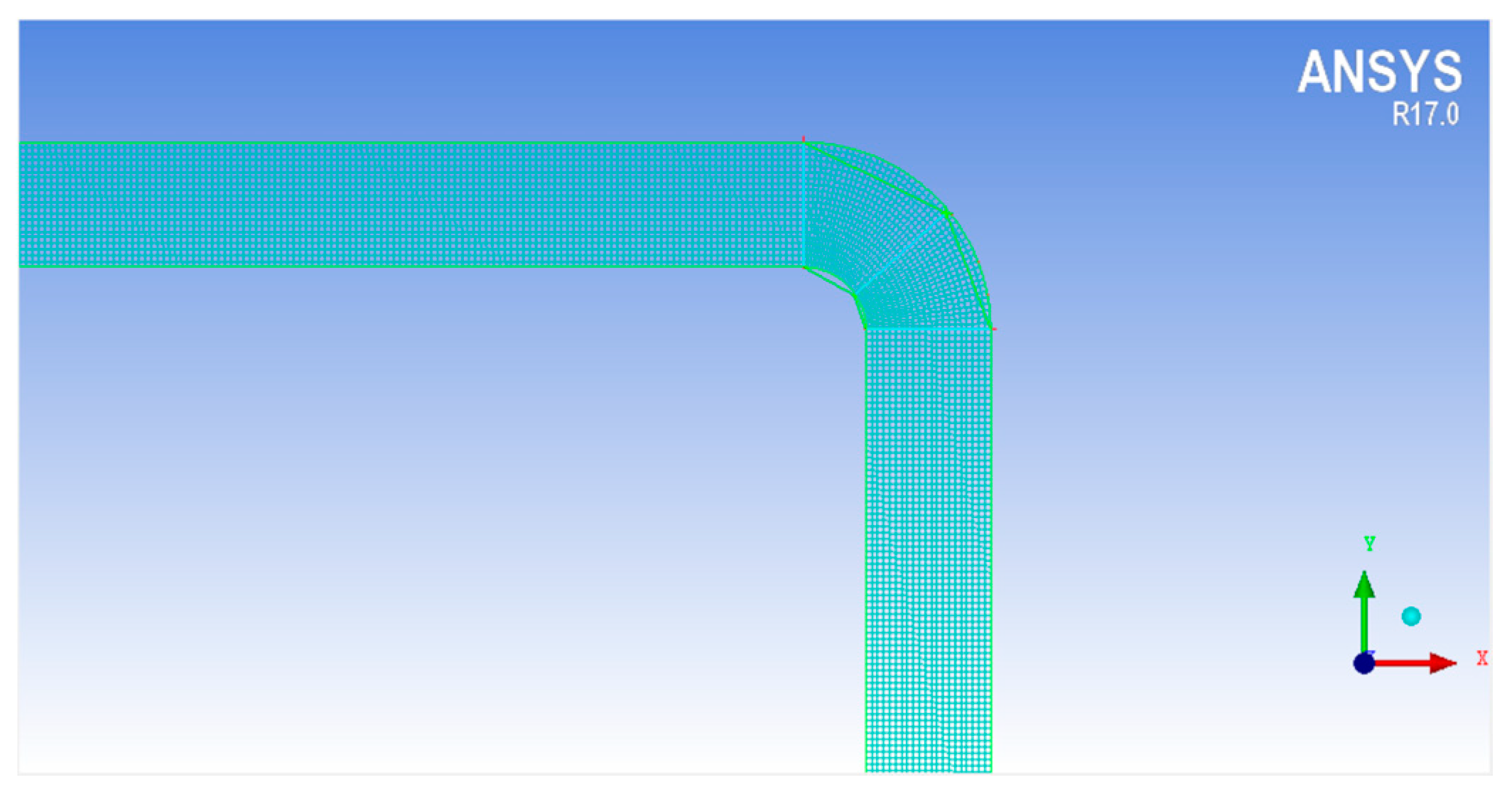
ANSYS 17.0 was used to generate the simplified 2D CFD model. There is no doubt that in simulation calculations, the accuracy of 2D simulation results is worse than that of 3D simulations. However, considering the hugeness of the DH network system, there is a high demand for simulation cost both in terms of calculation time and computational intensity. Therefore, the system was subjected to simulation. In order to obtain a high-quality mesh, a structural mesh was generated in the 2D CAD model, which can easily realize the boundary fitting of the region and is suitable for calculation of fluid and surface stress concentration. Structured meshes generate slower than unstructured meshes, but the number of structured meshes is much smaller than that of unstructured meshes, which can reduce computational intensiveness. The maximum mesh size was defined as 30 mm. In order to ensure the accuracy of the model, it was intended to increase the density of the mesh at the tee junction of the pipe. A partial view of the mesh from the heat source to the first elbow (see the red dotted ellipse area in Figure 1) is shown in Figure 2. The total number of meshes in the calculation domain is 252,7918.
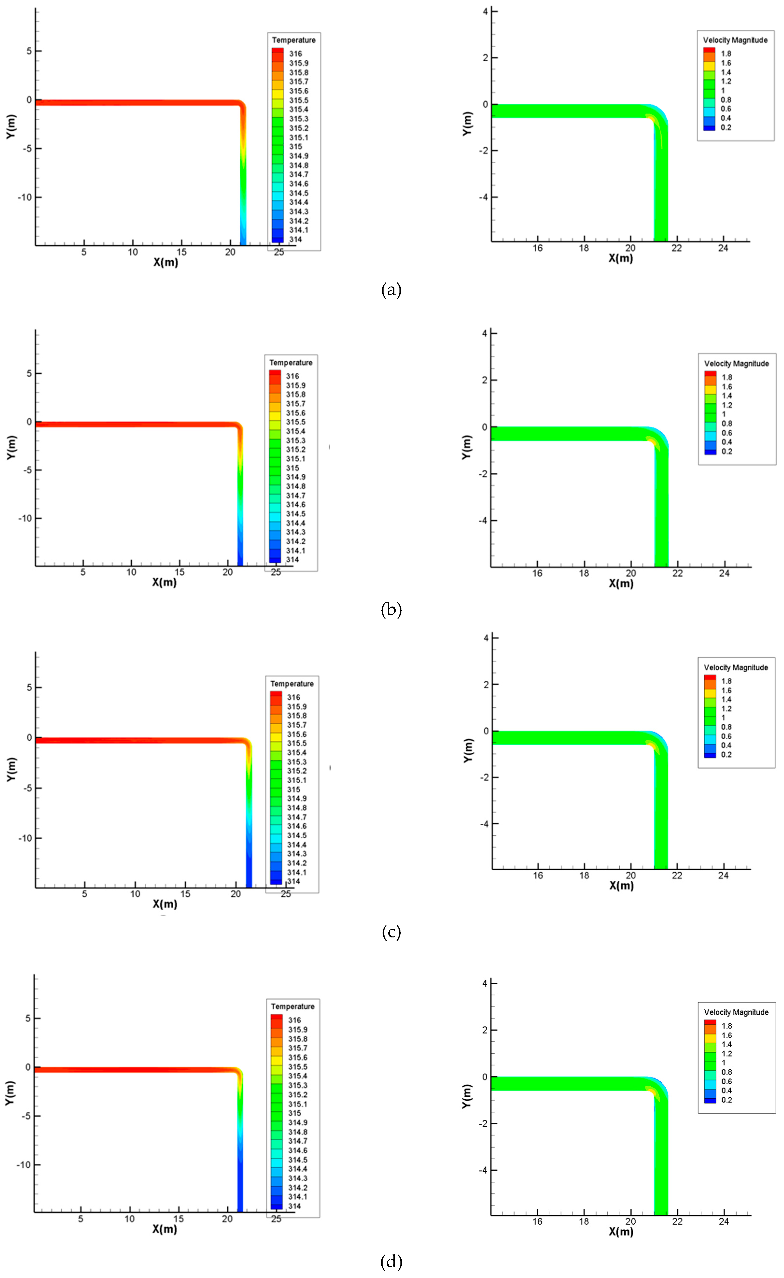
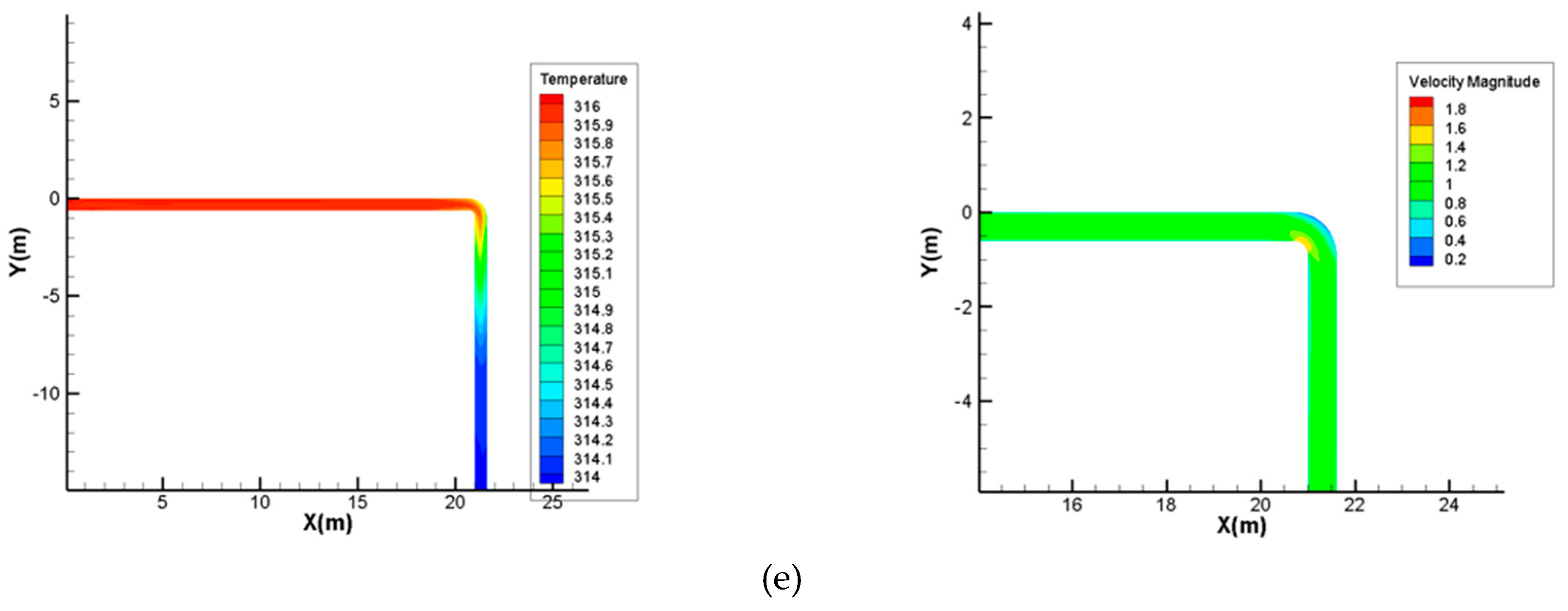
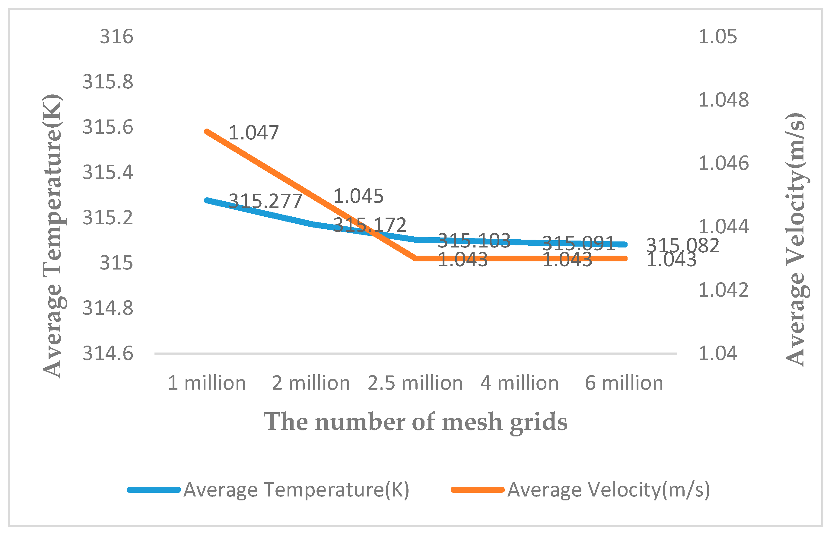
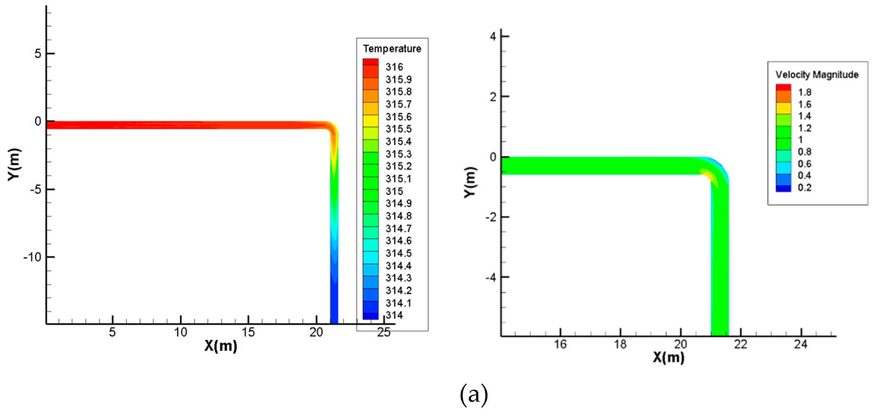
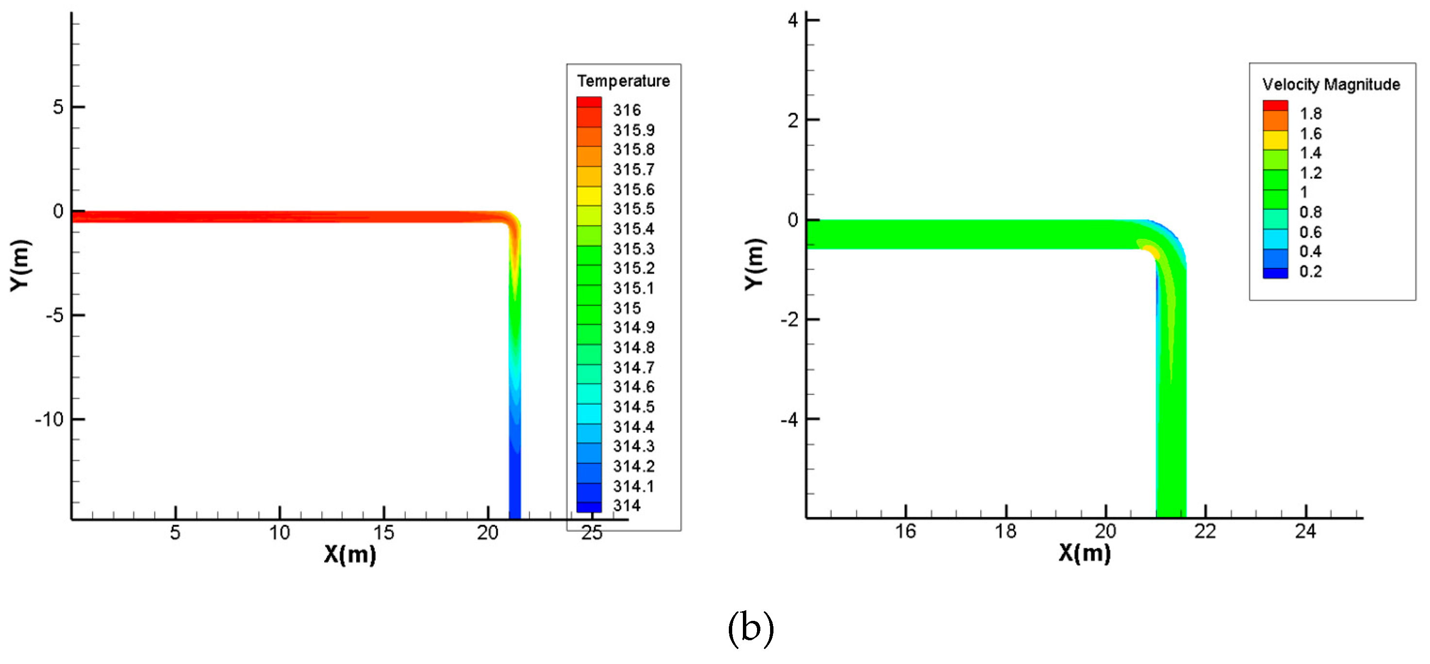
In order to prove the reasonableness and accuracy of the number of grids, the model needs to be verified for grid independent. The temperature and velocity contours comparisons from the heat source to the first elbow in five conditions of 1, 2, 2.5, 4 and 6 million are shown in Figure 3.
The test results of grid independence are shown in Figure 4. As can be seen from the grid independence results, when the number of grids reaches 2.5 million, the temperature and velocity changes will not be obvious. The computational cost and intensity are affected by the number of grids, and the computational cost increases as the number of grids increases. It is reasonable to have a grid number of 2.5 million.
In a large DH networks system, the temperature change of the supply water of the heat source takes a period of time to affect the heat consumers. This is the time delay due to changes in the water supply temperature. The Fluent solver was set up as a combination of steady-state calculations and transient calculations. The steady-state calculation makes the temperature in the DH network reach a certain value, and then the transient calculation was performed based on the steady state calculation to prove the influence of the water supply temperature change on the time delay of the DH network. The energy model was activated and the standard k-ε model equation was used as the turbulence model. Compared with the RNG model suitable for rotating flow calculation, the standard k-ε model is more suitable for solving the problem in this case. The turbulence governing equation is shown below:
where is the production term of turbulent energy k caused by average velocity gradient, is the production term of turbulent energy k caused by buoyancy, represents the contribution of pulsation expansion in compressible turbulence, For incompressible fluids, = 0. , , , and are empirical constants,, , , and , is fluid density, k is turbulent kinetic energy, is turbulent kinetic energy dissipation rate, u is fluid relative velocity, is fluid dynamic viscosity.
The SIMPLE algorithm was used as the pressure-velocity coupling method. The pressure discrete difference format uses the standard discrete difference format. For solving the flow problem, the other variables use the 1st upwind style. The 1st upwind is less accurate than the 2nd upwind, but it can make the steady-state calculation easier to converge, especially for this case. In order to improve the calculation accuracy, the 1st upwind convergence under steady-state conditions was used as the initial condition for the 2nd upwind transient calculation. The results of the comparison of the velocity and temperature profiles from the heat source to the first elbow are shown in Figure 5 when the momentum, turbulent model, and energy were discretized in 2nd order upward and 1st, respectively. The results show that it is reasonable to use the 1st upwind for steady-state calculations. The under-relaxation factors of pressure, density, momentum, turbulent kinetic energy, and energy were 0.3, 1, 0.7, 0.8 and 0.8, respectively. All of the given time steps are iteratively solved in a separate manner until the convergence condition was met. Two control monitors of the iterative process were defined to check convergence: a monitor for the residuals of the iterative process for the equations solved and the surface monitor of the outlet velocity. When the residual decreases at a value of 10-5, the simulation process was considered to be convergent. However, the oscillation occurs when the residual is calculated to be below 10-3. At this point, the surface monitor of the outlet velocity shows that the outlet velocity at this time remains constant, so the calculation is considered to have reached convergence. The Fluent 17.0 solver was calculated at steady state and the number of iterations is 4000. Another major step in CFD modeling was the establishment of boundary conditions. In the CFD model, the heat source and the heat consumers were defined as a velocity-inlet and pressure-outlet, respectively. The parameters of the boundary conditions were obtained from the measurements. Moreover, the wall of the pipe in the model was defined as an adiabatic wall to ignore the heat loss in the radial direction of the pipe.
After the steady state calculation converges, the temperature of the flow field in the model at this time reached the input temperature of the pipe velocity-inlet. Meanwhile, the Fluent 17.0 solver was subjected to transient calculations based on the steady-state simulation, with the temperature input of the velocity-inlet being changed. The second-order upwind space discretization algorithm was used for transient algorithms. Compared to first-order algorithms, second-order algorithms can achieve the best results because they can significantly reduce interpolation errors and false-value diffusion [21,22]. The time step size of the transient solver was set to 1s and the total time of the simulation was set to 4000 s. The maximum iterations were 20. The automatically save time for Fluent transient calculation was set to be automatically saved every 10 s. The temperature at each outlet of the DH network will vary with the input temperature of the velocity-inlet. The automatically saved Fluent data was read and analyzed the change of the temperature of the whole DH network system, which the time of the automatically saved Fluent data corresponding to each outlet temperature reaching the inlet temperature setting value to determine the time delay from the heat source to each consumer due to the temperature variation. By this method, the time delay of each heat consumer caused by the change in the water supply temperature of the heat source can be determined.
3.1.3. Boundary Conditions of the CFD Model
Boundary conditions need to be defined as part of the CFD model. In this case, the inlet and outlet of the model were set as the velocity-inlet and pressure-outlet, respectively. Parameters such as temperature and flow rate were obtained through experimental measurements and used as input parameters to define the boundary conditions.
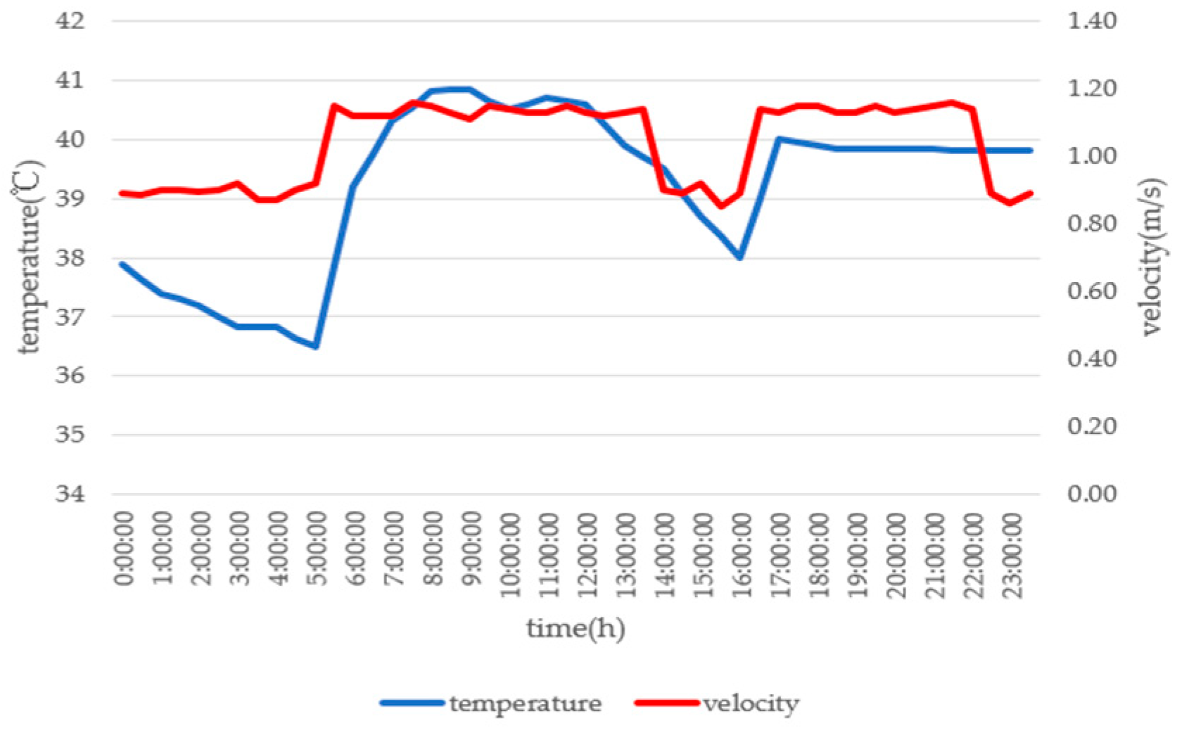
Temperature and flow measurements were performed at the supply pipe for the heat source and each heat consumer. The average of the supply water temperature and flow rate at the heat source were set as the inlet temperature and the inlet flow rate. The probe of the temperature recorder was installed on the water supply pipe at the heat source, and the water supply temperature was measured every 10 minutes. Similarly, the ultrasonic flowmeter was used to measure the flow rate of the water supply pipeline at the heat source every 10 minutes. The measured water supply temperature and flow rate at the heat source were shown in Figure 6. The average flow rate and water supply temperature at the heat source is 1.04 m/s and 39.2℃, which were used as a boundary condition for calculating the steady-state velocity-inlet of the CFD model. In the process of transient calculation, the velocity-inlet temperature was defined as 40.9℃ (The maximum temperature value on test day). In the CFD model, each consumer building heating entry was considered as an outlet, and the boundary condition of the outlet was defined as pressure-outlet. However, in an actual DH network system, the consumer building heating entry is not an outlet that is in communication with the atmosphere but rather has a pressure sufficient to provide hot water to the most unfavorable end of the building. This means that the pressure at the pressure-outlet cannot be set to 0 Pa. The outlet pressure can be obtained by reading the pressure gauge at the consumer building heating entry. A relative pressure of 0.4 MPa was defined as the input parameter of the pressure-outlet. The input parameters of the CFD model boundary conditions are shown in Table 2.
3.2. Equivalent Pipe Diameter
In the DH network, there is a strong coupling between the influencing parameters. The time delay of the heat consumer was determined by the combination of pipe length and pipe diameter. The diameter of the pipe from the heat source to the heat consumer is constantly changing with distance and is not a fixed value. In order to analyze the influence of various parameters on the time delay, complex practical engineering problems were transformed into ideal pipeline models. Therefore, the concept of equivalent pipe diameter () was proposed.
The pipe length is the superposition of the length of the heat medium flowing from the heat source to each consumer. The flow rate in the equivalent pipe diameter of each consumer is the flow rate to each consumer. Since pipe diameters are constantly changing along with the flow of heat medium, simple overlays summation is not possible. The equivalent pipe diameters () are defined based on practical frictional and local resistance. Under the same pipe length, the summation of the frictional resistance and local resistance of the heat medium from the heat source to the consumer through all the pipe sections is equivalent to a fixed pipe diameter of the single straight pipe, as Equation (6) shows. The fixed pipe diameter, namely the equivalent pipe diameter, can be calculated as Equation (7), which is derived from Equation (6):
where, is the frictional resistance (pa), is the local resistance (pa), L is the pipe length (m), v is the flow rate in each pipeline (m/s), ρ is the density of heat medium (kg/, λ is the friction coefficient, i is the pipe number and n is the total number of pipe sections.
The above Equation can calculate the equivalent diameter of each consumer in this case (see Section 4.3.3), and prepare for the subsequent parameter sensitivity analysis.
4. Results
4.1. A Solution of the CFD Model
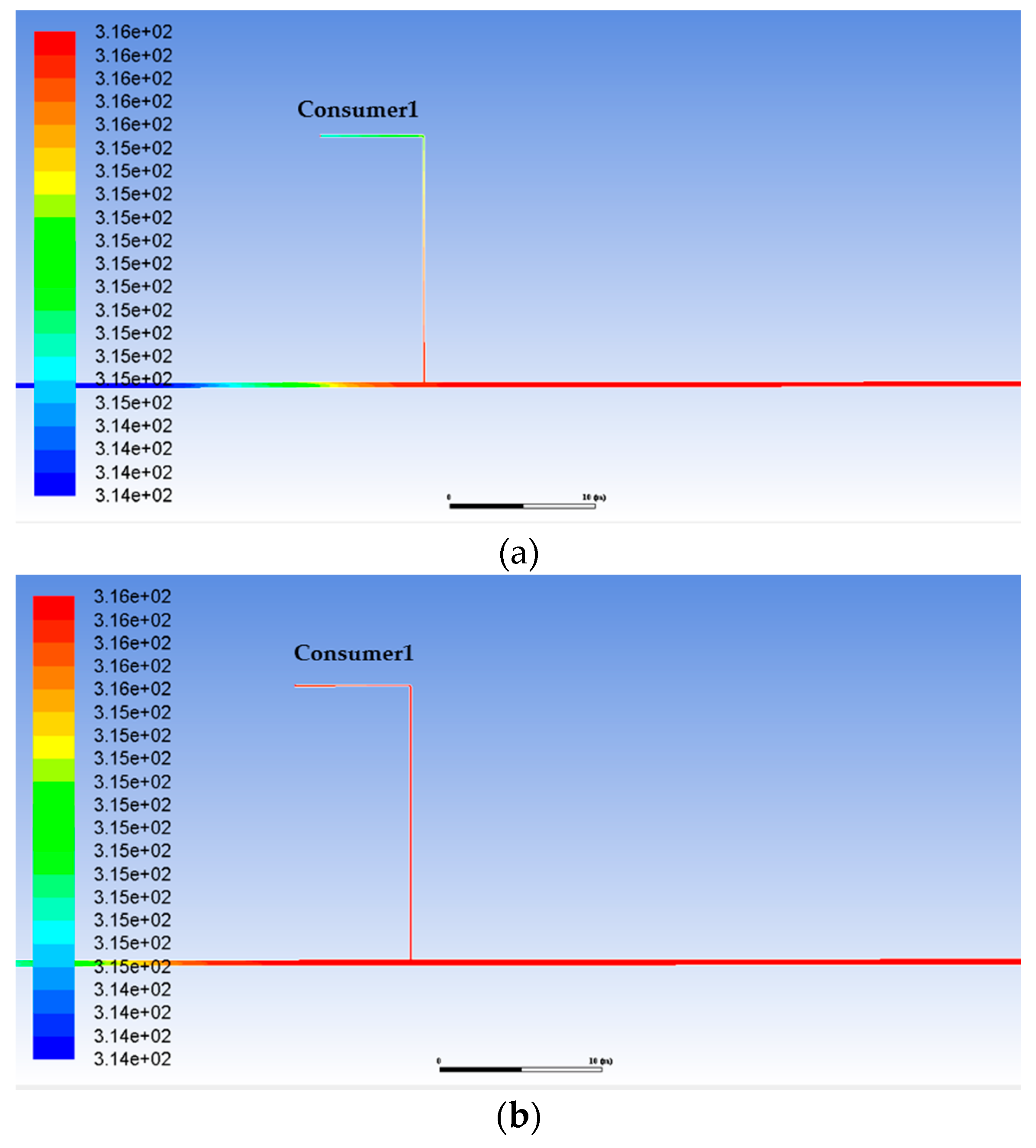
The steady state calculation results were used as initial conditions for transient calculations. The transient temperature change in the pipeline of the DH network system can be obtained by reading the temperature contours. As can be seen from Figure 7, taking Consumer 1 as an example, the temperature distribution in the pipeline ranges from 314.2 K to 315.9 K. 314.2 K is the temperature of the velocity-inlet under steady-state calculation, while the 315.9 K is the velocity-inlet temperature under transient simulation. Observe the change of the temperature band in the simulation result. When the temperature at the outlet reaches 315.9 K, the corresponding time is the time delay caused by the temperature change.
In Figure 7, the results represent the temperature at the build heating entry of Consumer 1 at 220 s and 240 s. As can be seen from the change of temperature of Figure 7a, the inlet temperature of the Consumer 1 reached 315 K at 220 s. However, from Figure 7b, we can see that the temperature of Consumer 1 has fully reached 315.9 K (the inlet temperature setting) at 240 s. Since the model is adiabatic and does not consider heat loss, it is considered that the time of setting temperature of the consumer inlet temperature is due to the time delay caused by the flow. The time delay of consumer1 is 240 s. Similarly, the time delay of other heat consumers can be obtained by reading the temperature contours of the simulation results. The time delay of other heat consumers is shown in Table 3.
4.2. Model Validation
4.2.1. Measurement Data
The correctness of the CFD model with variable temperature delay was verified based on the test data. The peak-valley method [23] was used to verify the correctness of the time delay. The temperature at the outlet of the heat consumer changes with the change of the inlet temperature of the heat source, and the temperature fluctuation curves of the two are consistent. The time corresponding to the peak and valley of the water supply temperature curve of the heat source and the inlet of each consumer was read separately. The difference in time between the peak (valley) of the heat source and the consumer is the time delay due to the change in the water supply temperature. Therefore, the water supply temperature of both the heat source and each of the heat consumers was measured.
A temperature recorder was installed on the water supply pipe of the heat source and the water supply pipe at the build heating entry of each heat consumer. The temperature of the water in the pipe was measured by the temperature probe of the temperature recorder and automatically recorded once every ten minutes.
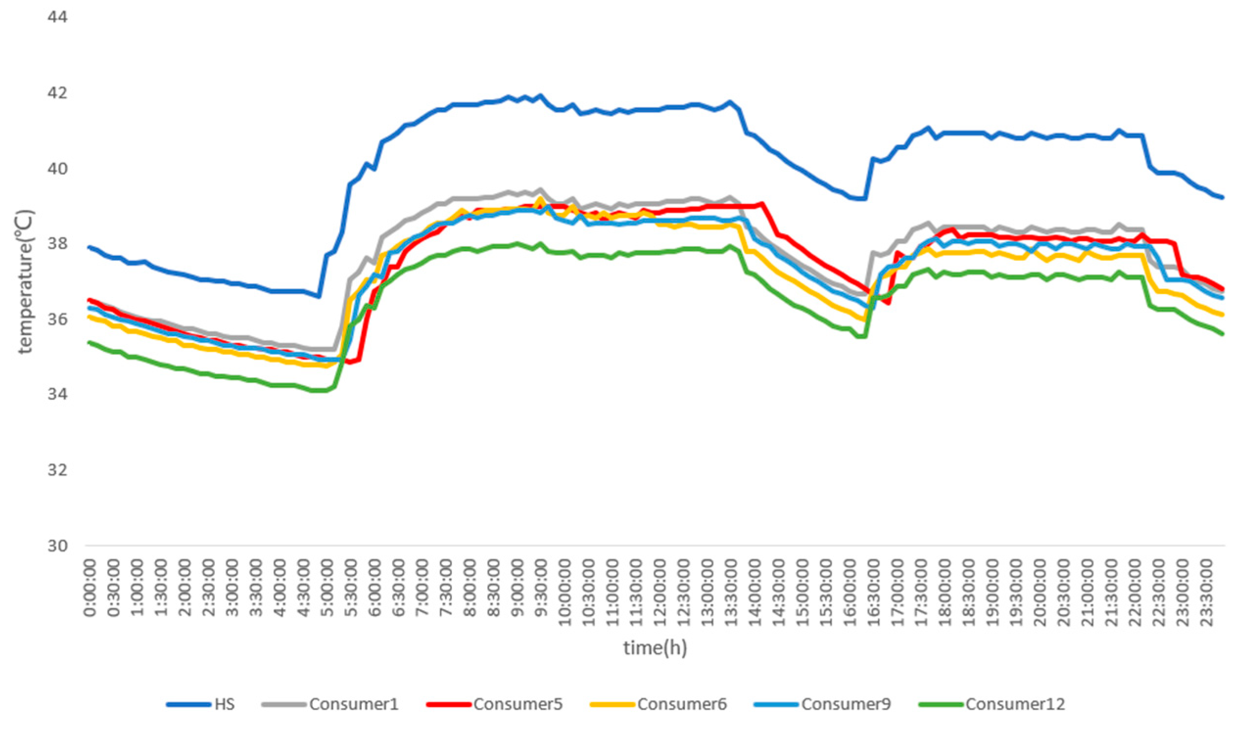
The hourly variation curve of water supply temperature at the HS and the consumer in one day is shown in Figure 8. The basic shapes of the hourly temperature curves are similar. The water temperature at the consumers changes after the water temperature changes at the heat source. The change of water temperature in the consumer lags behind the temperature of the water supply in the heat source.
Three days of test data were selected for model validation, with a total of six temperature peaks and six temperature valleys. The frequency statistics of the water supply temperature peak and valley of each consumer are shown in Table 4. The weighted average equation is as follows:
where, is the time delay of the weighted average (s), is the frequency of the time delay, ξ is the time delay (s).
The average time delay of each consumer can be calculated. The calculation results show the average time delay of each consumer: s 3650 s, s, 600 s.
4.2.2. Model Verification and Error Analysis
The calculation time delay with the test data and the time delay with the CFD model are shown in Table 5. In order to verify the accuracy of the model, relative error was introduced to compare two methods. As seen in Table 5, the results obtained by CFD model agree well with the test data. The maximum relative error is 7.14%. The minimum relative error is 0.29%. The correctness of the CFD model was proved by the result of a relative error.
The reasons for the error between the CFD model and the measured data are as follows:
- The CFD model was built based on the actual size of the system. However, due to the lack of data on some of the construction drawings, some pipelines are determined by the equivalent replacement method. During the actual construction process, the layout of the pipe network might end up being different from that described in the engineering data.
- The boundary condition of the CFD model based on test results may have some small gaps with the actual pipe network operation.
4.3. Parameter Sensitivity Analysis
4.3.1. Influencing Parameters
The time delay was defined as the time from when the inlet water temperature changes to the time when the pipe outlet water temperature begins to change. For fixed pipe insulation characteristics, the time delay is related to the distance of water flow and water velocity, while the distance of water flow is related to pipe length, and water velocity is related to flow and nominal diameter. In addition, the change in water supply temperature is another important parameter affecting the time delay. Therefore, the time delay of water temperature caused by hot water transmission in the main pipes and branch pipes is mainly affected by flow rate, pipe length, pipe diameter, and supply water temperature. The influence of four parameters on the time delay was studied, respectively.
4.3.2. Flow Rate
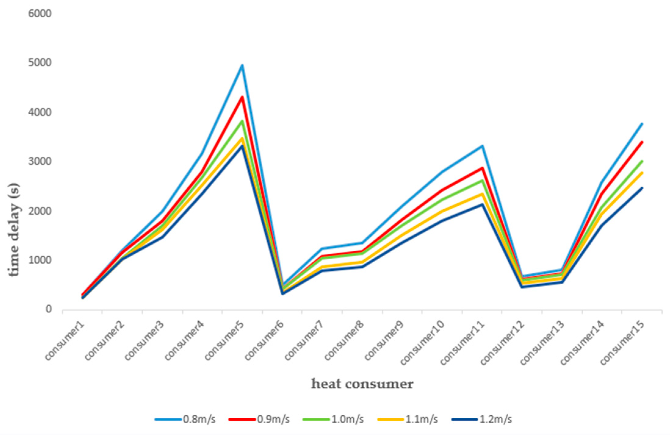
The time delay of each heat consumer in the actual case was obtained under the condition that the velocity-inlet is 1.04 m/s. The input flow rate at the velocity-inlet was changed to simulate under five working conditions of 0.8, 0.9, 1.0, 1.1 and 1.2 m/s, respectively, and the time delay of each heat consumer under five different flow rates was obtained. The time delay of each heat consumer under five different flow rates is shown in Figure 9. As can be seen from the simulation results, the time delay decreases as the flow rate increases. However, the time delay decreases rapidly at the beginning and then gradually slows down. This means that the change in time delay will no longer be apparent when the flow increases to a certain value. From the equation of resistance (see Equation (6)), it can be seen that the resistance is proportional to the square of the flow rate, and the resistance increases rapidly with the increase of the flow rate, which is the reason why the increase of the flow rate causes the rate of decrease of the time delay to continuously decrease.
4.3.3. Pipe Length and Pipe Diameter
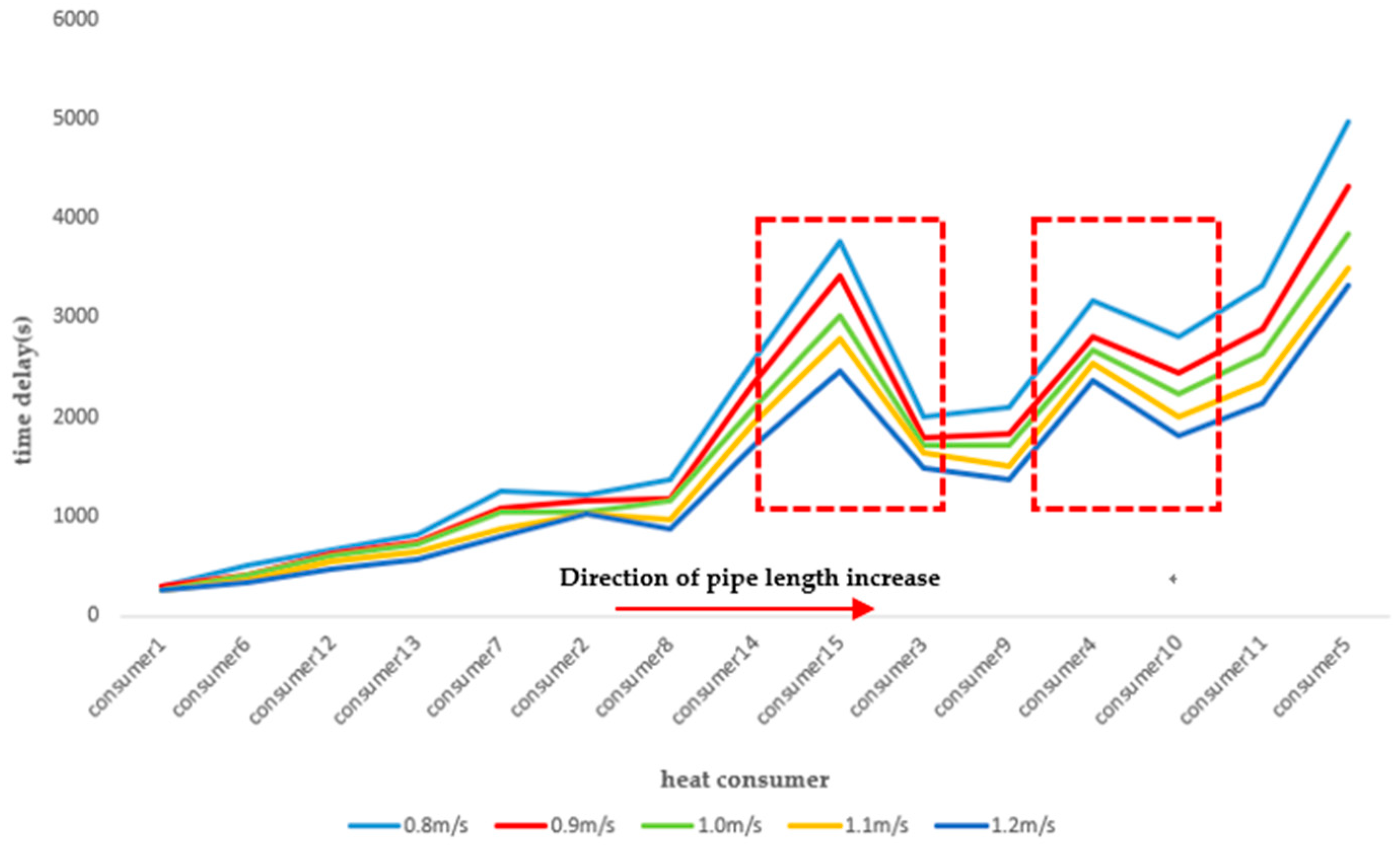
The relationship between the pipe length from the heat source to each heat consumer and the time delay is shown in Figure 10, where the abscissa represents the increase of the pipe length, from which it can be seen that the time delay of the heat consumer increases with the increases of pipe length. There are, however, two distinct breaks in the curve. The reason for this phenomenon is that the research on the relationship between the time delay of each heat consumer and the pipe length was not carried out under the condition of the same pipe diameter. The equivalent pipe diameter of each heat consumer was calculated by Equations (6) and (7). The calculation results of pipe length, equivalent pipe diameter, and flow rate are shown in Table 6.
The pipe length of heat Consumer 3 is greater than that of heat Consumer 15, but the time delay of heat Consumer 15 is greater than that of Consumer 3 because the equivalent pipe diameter of heat Consumer 15 is greater than that of heat Consumer 3. Similarly, the heat Consumer 10 has a larger pipe length than the heat Consumer 4, but its diameter is smaller than that of the heat Consumer 4. It can be seen that the influencing factors of the time delay of the DH network system are the result of the combined effect of pipe diameter and pipe length. The sensitivity analysis results of pipe length and pipe diameter are shown in Table 7. It can be seen from Table 7 that the effect of pipe diameter on the time delay of each heat consumer is greater than that of pipe length.
4.3.4. Supply Water Temperature
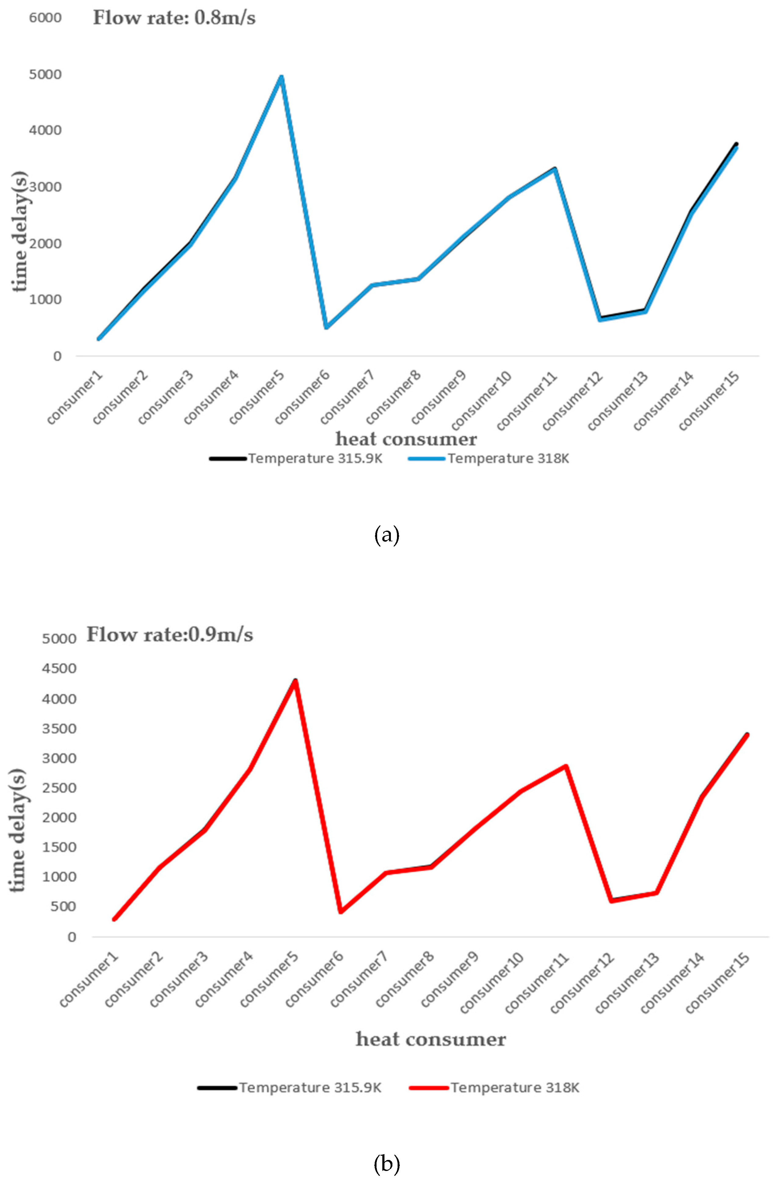
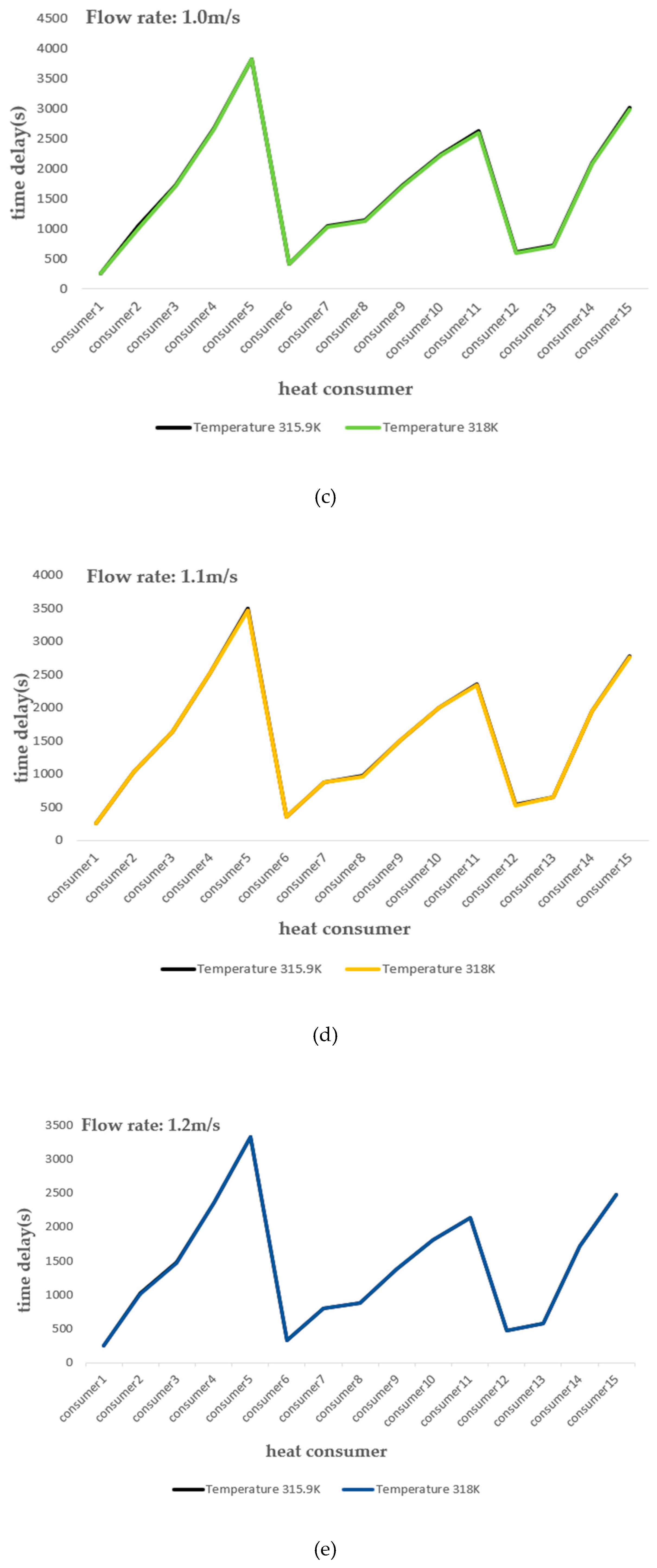
In the actual case, the water supply temperature changed from 314.2 K to 315.9 K. In order to prove whether the time delay of each heat consumer is related to the value of water supply temperature change, the input temperature of velocity-inlet of CFD model needs to be changed. Therefore, the temperature of the velocity-inlet was changed from 315.9 K to 318 K for transient simulation. The two water supply temperatures were simulated separately under five different flow rate conditions, and the obtained time delay of each heat consumer was shown in Figure 11a–e.
It can be seen from the simulation results that the change of the water supply temperature has little effect on the time delay. The time delay of each heat consumer is almost the same before and after changing the water supply temperature for both the DH network system with large flow rate (1.2 m/s) and the DH network system with small flow rate (0.8 m/s). However, the fitting degree of the two temperature curves of the DH network system with a large flow rate is higher than that of the DH network system with a small flow rate. It means that the change of water supply temperature has a greater impact on the DH network system with a small flow rate than the DH network system with a large flow rate. The reason for the analysis is that the inlet water temperature rises to make the water temperature in the pipeline higher, and the high water temperature is favorable for accelerating heat transfer. Therefore, the time delay is shortened when the inlet water temperature changes.
5. Discussion
According to the parameter sensitivity analysis, the time delay of each heat consumer is different for the DH network system, which proves that the time delay of each heat consumer was affected by the interaction of various influencing parameters. In order to regulate and optimize the DH network system, the relationship between the time delay of each heat consumer and the influence parameters in the DH network system must be considered. The CFD simulation method proposed in this paper can calculate the time delay of the established DH system and be applied to the control operation of the DH network system. Therefore, the analysis of the time delay of each heat consumer is very important and meaningful for the implementation of the control strategy of the DH network system.
The water in the DH network is regarded as an incompressible fluid, and the change of flow and pressure at the inlet can be regarded as a non-delayed response to the terminal. However, under the influence of the combined effects of flow and heat transfer, the temperature has a certain time delay response to the terminal, which is a dynamic response problem. This paper only analyzes the influence parameters of time delay under the static working condition through the change of boundary conditions. Based on the CFD model established in this paper, the dynamic response of the DH network after temperature change will continue to be deeply analyzed in the future.
The CFD method was used to obtain the time delay of each heat consumer of the DH network system and they can provide services for the optimization of the control strategy. However, the CFD method was limited to computation time and intensity. The current simulation is suitable for the small-scale DH network systems without any range limitation of temperature and flow rate. For large-scale DH network systems, the computational cost will also increase. In addition, this method only provides an idea to simulate the calculation of the system time delay at the time when the flow rate and temperature at the heat source are constant. The method is limited for the calculation of the time delay of the system where the temperature and flow rate of the heat source is constantly changing.
6. Conclusions
A model based on the CFD method to determine the time delay of the DH network was proposed. By changing the boundary conditions of the CFD model, the influence parameters of the DH network time delay were analyzed. The different time delay of each heat consumer is due to the combined effect of various influencing parameters. The results show that the flow rate, pipe length and pipe diameter have a significant impact on the time delay of the DH network system.
The increase in the operating flow rate of the DH network system can reduce the time delay of each heat consumer. However, when the flow rate increases to a certain value, the reduction of time delay will no longer be obvious. The time delay of the DH network system is proportional to the change in pipe length and pipe diameter. The pipe diameter has a greater impact on the time delay of the DH network system than the effect of the pipe length. The water supply temperature has little effect on the time delay of the DH network system. The time delay before and after the water supply temperature change in the DH network system is almost the same.
In the future, the proposed method can simulate the CFD model to calculate the time delay of the DH network system. Compared to other simulation methods and mathematical methods, the method can quickly calculate the time delay of the DH network system under different operating parameters by changing the boundary conditions. The relationships between the influencing parameters and the time delay are very important for the control strategy of the DH network system. The time delay obtained by the CFD method is of great significance for the implementation of the operation control strategy of the DH network system and the reduction of system energy consumption. The calculation method of time delay is potential research for the optimization control of the DH network system in the future.
Author Contributions
Methodology, J.Z.; Software, Y.S.; Validation, Y.S. Formal Analysis, J.Z.; Investigation, J.Z.; Resources, J.Z.; Writing-Original Draft Preparation, Y.S.; Writing-Review & Editing, Y.S.
Acknowledgments
This research was supported by Natural Science Foundation of China, Project No. 51678398 and the Natural Science Foundation of Tianjin, Project No.18JCQNJC08400.
Conflicts of Interest
The authors declare no conflict of interest.
References
- Lund, H.; Möller, B.; Mathiesen, B.V.; Dyrelund, A. The role of district heating in future renewable energy systems. Energy 2010, 35, 1381–1390. [Google Scholar] [CrossRef]
- Persson, U.; Werner, S. Heat distribution and the future competitiveness of district heating. Appl. Energy 2011, 88, 568–576. [Google Scholar] [CrossRef]
- Xu, Y.C.; Chen, Q. An entransy dissipation-based method for global optimization of district heating networks. Energy Build. 2011, 43, 50–60. [Google Scholar] [CrossRef]
- Neuman, P.; Pokorny, M.; Weiglhofer, W. Principles of Smart Grids on the generation electrical and thermal energy and control of heat consumption within the District Heating Networks. IFAC Proc. Vol. 2014, 47, 1–6. [Google Scholar] [CrossRef]
- Benonysson, A.; Bøhm, B.; Ravn, H.F. Operational optimization in a district heating system. Energy Convers. Manag. 1995, 36, 297–314. [Google Scholar] [CrossRef]
- Sartor, K. Experimental validation of heat transport modeling in district heating networks. In Proceedings of the 29th International Conference on Efficiency, Cost, Optimisation Simulation and Environmental Impact of Energy Systems (ECOS 2016), Portorož, Slovenia, 19–23 June 2016. [Google Scholar]
- Wang, N.; You, S.J.; Zheng, W.D.; Zhang, H.; Zheng, X.J. A Simple Thermal Dynamics Model and Parameter Identification of District Heating Network. Procedia Eng. 2017, 205, 329–336. [Google Scholar] [CrossRef]
- Pirouti, M.; Bagdanavicius, A.; Ekanayake, J.; Wu, J.; Jenkins, N. Energy consumption and economic analyses of a district heating network. Energy 2013, 57, 149–159. [Google Scholar] [CrossRef]
- Hong, S.L.; Kim, G. Prediction model of Cooling Load considering time-lag for preemptive action in buildings. Energy Build. 2017, 155, 53–65. [Google Scholar]
- Li, X.M.; Zhao, T.Y.; Zhang, J.L. Predication control for indoor temperature time-delay using Elman neural network in variable air volume system. Energy Build. 2017, 154, 545–552. [Google Scholar] [CrossRef]
- Jie, P.F.; Tian, Z.; Yuan, S.S.; Zhu, N. Modeling the dynamic characteristics of a district heating network. Energy 2012, 39, 126–134. [Google Scholar] [CrossRef]
- Zheng, J.F.; Zhou, Z.G.; Zhao, J.N.; Wang, J.D. Function method for dynamic temperature simulation of a district heating network. Appl. Therml. Eng. 2017, 123, 682–688. [Google Scholar] [CrossRef]
- Wang, H.; Meng, H. Improved thermal transient modeling with new 3-order numerical solution for a district heating network with consideration of the pipe wall’s thermal inertia. Energy 2018, 160, 171–183. [Google Scholar] [CrossRef]
- Li, L.; Zaheeruddin, M. A control strategy for energy optimal operation of a direct district heating system. Int. J. Energy Res. 2004, 28, 597–612. [Google Scholar] [CrossRef]
- Sartor, K.; Thomas, D.; Dewallef, P. A comparative study for simulation of heat transport in large district heating network. In Proceedings of the 28th International Conference on Efficiency, Cost, Optimization, Simulation and Environmental Impact of Energy Systems (Ecos2015), Pau, France, 29 June–3 July 2015; Volume 56, pp. 174–180. [Google Scholar]
- Gabrielaitiene, I.; Sunden, B.; Kacianauskas, R.; Bohm, B. Dynamic modelling of the thermal performance of district heating pipelines. Am. J. Physiol. 2003, 211, 95–98. [Google Scholar]
- Palsson, H.; Larsen, H.V.; Ravn, H.F.; Bohm, B.; Zhou, J. Equivalent Models of District Heating Systems; Technical University of Denmark and Risø National Laboratory: Roskilde, Denmark, 1999. [Google Scholar]
- Gabrielaitiene, I.; Bøhm, B.; Sunden, B. Modelling temperature dynamics of a district heating system in Naestved, Denmark—A case study. Energy Convers. Manag. 2007, 48, 78–86. [Google Scholar] [CrossRef]
- Vesterlund, M.; Toffolo, A.; Dahl, J. Simulation and analysis of a meshed district heating network. Energy Convers. Manag. 2016, 122, 63–73. [Google Scholar] [CrossRef]
- Liu, X.; Ge, X.F. FLUENT software and its application in China. Energy Res. Util. 2003, 02, 36–38. [Google Scholar]
- Ferziger, J.H.; Peric, M. Computational methods for fluid dynamics. Phys. Today 1997, 50, 80–84. [Google Scholar] [CrossRef]
- Blazek, J. Computational Fluid Dynamics: Principles and Applications; Elsevier: Oxford, UK, 2001; Volume 55, pp. 1–496. [Google Scholar]
- Östlund, K.; Samuelsson, C.; Mattsson, S.; Rääf, C.L. The influence of 134Cs on the 137Cs gamma-spectrometric peak-to-valley ratio and improvement of the peak-to-valley method by limiting the detector field of view. Appl. Radiat. Isotopes 2017, 128, 249–255. [Google Scholar] [CrossRef] [PubMed]
Figure 1.
The district heating network in Tianjin University.

Figure 2.
The local mesh of the CFD model.

Figure 3.
(a) Temperature contours and velocity contours under 1 million grids; (b) Temperature contours and velocity contours under 2 million grids; (c) Temperature contours and velocity contours under 2.5 million grids; (d) Temperature contours and velocity contours under 4 million grids; (e) Temperature contours and velocity contours under 6 million grids.


Figure 4.
The test results of grid independence.

Figure 5.
(a) Temperature contours and velocity contours in 1st order upward; (b) Temperature contours and velocity contours in 2nd order upward.
Figure 5.
(a) Temperature contours and velocity contours in 1st order upward; (b) Temperature contours and velocity contours in 2nd order upward.


Figure 6.
The measured temperature and velocity at HS.

Figure 7.
(a) The temperature of Consumer 1 at 220 s; (b) the temperature of Consumer 1 at 240 s.

Figure 8.
Hourly water supply temperature at HS and consumer.

Figure 9.
The time delay of each heat consumer under five different flow rates.

Figure 10.
The relationship between the pipe length and the time delay of each heat consumer.

Figure 11.
(a) Comparison of the time delay obtained by the two different temperature simulations under the condition of 0.8 m/s; (b) Comparison of the time delay obtained by the two different temperature simulations under the condition of 0.9 m/s; (c) Comparison of the time delay obtained by the two different temperature simulations under the condition of 1.0 m/s; (d) Comparison of the time delay obtained by the two different temperature simulations under the condition of 1.1 m/s; (e) Comparison of the time delay obtained by the two different temperature simulations under the condition of 1.2 m/s.


Table 1.
Building function and distance from the heat source about each consumer.
| Consumer | Building Function | Distance from the Heat Source (m) |
|---|---|---|
| Consumer 1 | Information and network center | 145.00 |
| Consumer 5 | teaching building 44 | 633.00 |
| Consumer 6 | library | 156.00 |
| Consumer 9 | laboratory building | 451.10 |
| Consumer 12 | teaching building 46 | 179.00 |
Table 2.
The input parameters of the CFD model boundary conditions.
| Steady State | Transient | ||
|---|---|---|---|
| Velocity-inlet | Flow rate (m/s) | 1.04 | 1.04 |
| Temperature (K) | 314 | 316 | |
| Pressure-outlet | Pressure (MPa) | 0.4 | 0.4 |
Table 3.
The delay time of the heat consumer.
| Consumer | Time Delay (s) | Distance from Heat Source (m) |
|---|---|---|
| 1 | 240 | 145.00 |
| 2 | 1040 | 339.00 |
| 3 | 1720 | 439.70 |
| 4 | 2680 | 514.30 |
| 5 | 3830 | 633.00 |
| 6 | 420 | 156.00 |
| 7 | 1050 | 316.00 |
| 8 | 1150 | 339.60 |
| 9 | 1720 | 451.10 |
| 10 | 2240 | 534.10 |
| 11 | 2630 | 563.10 |
| 12 | 610 | 179.00 |
| 13 | 720 | 204.20 |
| 14 | 2090 | 367.80 |
| 15 | 3010 | 420.60 |
Table 4.
Frequency statistics of the time delay of consumers.
| Consumer | Time Delay (s) | Water Temperature Valley | Water Temperature Peak |
|---|---|---|---|
| 210 | 1 | 0 | |
| Consumer 1 | 240 | 4 | 5 |
| 300 | 1 | 1 | |
| 3300 | 1 | 0 | |
| Consumer 5 | 3600 | 4 | 4 |
| 3900 | 1 | 2 | |
| 420 | 4 | 4 | |
| Consumer 6 | 480 | 2 | 1 |
| 600 | 0 | 1 | |
| 1500 | 1 | 0 | |
| Consumer 9 | 1680 | 3 | 2 |
| 1800 | 2 | 4 | |
| 300 | 3 | 1 | |
| Consumer 12 | 600 | 2 | 2 |
| 900 | 2 | 2 |
Table 5.
Comparison of the CFD method with the peak-valley method.
| Consumer | The Time Delay Calculated by the CFD Method (s) | The Time Delay Calculated by the Peak-Valley Method (s) | Relative Error |
|---|---|---|---|
| Consumer 1 | 240 | 245 | 2.08% |
| Consumer 5 | 3830 | 3650 | 4.70% |
| Consumer 6 | 420 | 450 | 7.14% |
| Consumer 9 | 1720 | 1725 | 0.29% |
| Consumer 12 | 610 | 600 | 1.64% |
Table 6.
Correlation pipeline parameters of each consumer.
| Consumer | Time Delay (s) | Pipe Length (m) | Equivalent Pipe Diameter (mm) | Flow Rate (m3/h) |
|---|---|---|---|---|
| 1 | 240 | 145.00 | 159.2 | 38.07 |
| 2 | 1040 | 339.00 | 155.7 | 24.08 |
| 3 | 1720 | 439.70 | 192.4 | 41.80 |
| 4 | 2680 | 514.30 | 208.4 | 56.66 |
| 5 | 3830 | 633.00 | 231.8 | 69.80 |
| 6 | 420 | 156.00 | 289.6 | 126.89 |
| 7 | 1050 | 316.00 | 164 | 30.02 |
| 8 | 1150 | 339.60 | 174.5 | 33.51 |
| 9 | 1720 | 451.10 | 181.2 | 37.23 |
| 10 | 2240 | 534.10 | 135.1 | 19.82 |
| 11 | 2630 | 563.10 | 258.8 | 78.42 |
| 12 | 610 | 179 | 151.1 | 31.11 |
| 13 | 720 | 204.2 | 153 | 32.28 |
| 14 | 2090 | 367.8 | 232.9 | 82.29 |
| 15 | 3010 | 420.6 | 246.4 | 57.02 |
Table 7.
Sensitivity analysis of pipe length and pipe diameter.
| Variable Parameters | Variation Rate of Parameters (%) | Time Delay to Each Heat Consumer (s) | ||||
|---|---|---|---|---|---|---|
| Consumer 1 | Consumer 5 | Consumer 6 | Consumer 9 | Consumer 12 | ||
| d | −20 | 150 | 2530 | 270 | 1100 | 390 |
| −10 | 180 | 3080 | 310 | 1380 | 460 | |
| 0 | 240 | 3830 | 420 | 1720 | 610 | |
| 10 | 280 | 4600 | 490 | 2060 | 720 | |
| 20 | 330 | 5500 | 580 | 2470 | 850 | |
| L | −20 | 180 | 3010 | 320 | 1340 | 470 |
| −10 | 200 | 3420 | 350 | 1530 | 520 | |
| 0 | 240 | 3830 | 420 | 1720 | 610 | |
| 10 | 260 | 4120 | 460 | 1870 | 670 | |
| 20 | 280 | 4590 | 490 | 2060 | 720 | |
© 2019 by the authors. Licensee MDPI, Basel, Switzerland. This article is an open access article distributed under the terms and conditions of the Creative Commons Attribution (CC BY) license (http://creativecommons.org/licenses/by/4.0/).
Share and Cite
MDPI and ACS Style
Zhao, J.; Shan, Y. An Influencing Parameters Analysis of District Heating Network Time Delays Based on the CFD Method. Energies 2019, 12, 1297. https://0-doi-org.brum.beds.ac.uk/10.3390/en12071297
AMA Style
Zhao J, Shan Y. An Influencing Parameters Analysis of District Heating Network Time Delays Based on the CFD Method. Energies. 2019; 12(7):1297. https://0-doi-org.brum.beds.ac.uk/10.3390/en12071297
Chicago/Turabian StyleZhao, Jing, and Yu Shan. 2019. "An Influencing Parameters Analysis of District Heating Network Time Delays Based on the CFD Method" Energies 12, no. 7: 1297. https://0-doi-org.brum.beds.ac.uk/10.3390/en12071297
Note that from the first issue of 2016, this journal uses article numbers instead of page numbers. See further details here.