Concatenate Convolutional Neural Networks for Non-Intrusive Load Monitoring across Complex Background

Abstract

Non-Intrusive Load Monitoring (NILM) provides a way to acquire detailed energy consumption and appliance operation status through a single sensor, which has been proven to save energy. Further, besides load disaggregation, advanced applications (e.g., demand response) need to recognize on/off events of appliances instantly. In order to shorten the time delay for users to acquire the event information, it is necessary to analyze extremely short period electrical signals. However, the features of those signals are easily submerged in complex background loads, especially in cross-user scenarios. Through experiments and observations, it can be found that the feature of background loads is almost stationary in a short time. On the basis of this result, this paper provides a novel model called the concatenate convolutional neural network to separate the feature of the target load from the load mixed with the background. For the cross-user test on the UK Domestic Appliance-Level Electricity dataset (UK-DALE), it turns out that the proposed model remarkably improves accuracy, robustness, and generalization of load recognition. In addition, it also provides significant improvements in energy disaggregation compared with the state-of-the-art.

1. Introduction

Energy consumption has always been a major concern in the world, which can be alleviated with accurate and efficient load monitoring methods. There are two branches of load monitoring, namely intrusive load monitoring (ILM) and non-intrusive load monitoring (NILM). The major difference between them is the number of sensors. The ILM needs to install at least one sensor at each appliance to monitor the load respectively, while the NILM needs to install one sensor on the bus per house merely. The NILM is physically simple at the cost of more complex approaches, thus NILM based approaches are more widely researched.

NILM contains two main objectives: energy disaggregation and load recognition. Conventional energy disaggregation aims to obtain energy consumption for every single appliance, which acts on the entire operation cycle of an appliance, and some research discards event detection and gives a result at the hour level to disaggregate the energy consumption [1]. The approximate power consumption of each appliance in a certain period is its main concern, thus the exact on/off time of appliances is unknown. For online load recognition, appliances are detected from the uncompleted operation cycle, that is the transient-state process of on/off events. In addition, the result of load recognition further benefits energy disaggregation. Some advanced applications in the smart grid need to acquire appliance operation status for remote household control [2], such as demand response. It represents that the power supply side uses induction mechanism (e.g., price changes over time) to improve end users’ energy consumption patterns, which demands for the balance of demand and supply in real time [3].

Real-time load recognition requires short sample windows and short execution time. The sample window is usually in seconds, while the execution time is less than a second. Obviously the former has a more significant impact on real time, thus the transient-state process should be captured and recognized. High sampling rate is necessary for sufficient information acquisition from transient-state features. High enough frequency (i.e., 100 kHz or higher) features can easily distinguish different appliances (e.g., electromagnetic interference (EMI) signatures), but EMI features can only be transmitted within a few meters, which is not suitable for household or industrial use. This paper uses 2 kHz features, which introduces interference from background loads, so the emphasis of this paper is to eliminate the influence of complex background loads. There are diverse types of appliances in different houses, and even the same type of appliances in different households vary by brand. It is hard for researchers to collect all combinations of appliances. Briefly, household electrical signals are multi-source single-channel data. Several similar topics are raised at the task of multi-source signals processing, such as the cocktail party problem in speech recognition and blind source separation (BSS) in wireless communications. Multichannel observations are necessary in these areas, whether it is two-channel audio-visual data [4] or two-channel audio observed signal [5], the data source itself gives the possibility of separation. Noiseless samples are used for training and being compared with separated samples in speech recognition methods, and artificial communication signals have the property of time or frequency separability, or they are orthogonal to each other. Unlike these problems, people can hardly obtain individual appliance samples in the single-channel scenario by non-intrusive approaches. To extract the feature of the target appliance from the load mixed with background loads, this paper utilizes the fact that the electrical signal is approximately stationary in a short time, in other words, loads are strongly correlated during this period.

Due to the powerful feature extraction ability of deep learning, this paper proposes an efficient network called the concatenate convolutional neural network. The model combines signal processing and pattern recognition to eliminate the influence of background loads in single-channel data and recognize different appliances. Features in high-dimensional spectrograms can be extracted in virtue of the development of deep neural networks. A series of deep convolutional networks for image classification have been proposed, such as Extreme Inception (Xception) [6], Residual Net (ResNet) [7], Dense Convolutional Network (DenseNet) [8]. In this paper, high-frequency current data is converted to spectrograms by Short Time Fourier Transform (STFT) and set as the model input. Two proven networks are used as the embedding layer to extract spectrogram features. However, it is problematic to apply object recognition methods to the model input without modification. The recognition object covers the background in computer vision, thus the background causes little substantial impact of recognition, whereas the foreground appliance in spectrograms suffers from blurring due to the superimposition of background loads.

The main contributions of this paper are as follows. (1) The model eliminates the impact of background loads to a certain extent, and achieves an F1-score of 89.0% in the classification task. (2) The proposed approach improves the performance of energy disaggregation, especially on multi-state appliances and programmable appliances. It increases an F1-score of 3–73% and reduces mean square error (MAE) of 3.1–24.2 watts. The proposed model is evaluated on the UK Domestic Appliance-Level Electricity dataset (UK-DALE) [9] and the Building-Level fUlly labeled dataset for Electricity Disaggregation (BLUED) [10]. The proposed model is also compared with several works in the aspect of energy disaggregation. In the remainder of this paper, the research status of NILM and the proposed network model will be introduced. Next, the results of the classification and energy disaggregation experiments are presented. Finally, this paper provides conclusions and future work.

2. Related Work

NILM was proposed by Hart more than 20 years ago [11], and numerous related research projects have begun since then. In the demand side management (DSM) program, the home energy management system comprises active appliances and passive appliances [12]. The active appliances consist of energy sources and energy storage systems [13,14]. Like most NILM methods, passive appliances are only considered in this paper. The approaches of improving classification accuracy or energy disaggregation results are closely related to data acquisition and feature selection.

The sampling rate in data acquisition can be simply divided into high-frequency and low-frequency, which directly affects the selection of features and approaches. Low-frequency data is typically used for approaches based on steady-state features, whereas high-frequency data is used for the transient-state analysis. Low-frequency data is easy to acquire and suitable for energy disaggregation [15,16]. The fundamental frequency is either 50 Hz or 60 Hz in most countries, thus sampling at several Hertz or lower is not suitable for spectrum analysis. High-frequency sampling at over 1 kHz captures features of higher harmonics and further recognizes different loads. Prior work [17] proved that the power spectrum computed from 15 kHz transient-state data can identify different loads with the same steady-state active and reactive power.

The higher the sampling frequency, the richer the information obtained. Multiple appliances could be distinguished by high-frequency signatures. Previous research showed that when the sampling rate was as high as 1 MHz, the EMI signatures of almost all appliances were distinguishable on the spectrograms [18], but the signatures could not be transmitted over a long distance, even in tens of square meters house. Low-noise data with no background load has been measured in some datasets [19,20], so there is no need to address these problems with complex networks.

In the field of power, the features are almost directly or indirectly derived from current, voltage, and power. These features in time domain or frequency domain are used in various methods, which mainly focus on some common machine learning algorithms, such as support vector machine (SVM) [21], k-nearest neighbors (kNN) [21], decision tree [22], wavelet design [23], evolutionary algorithm [24], adaptive boost [24], graph signal processing (GSP) [25], hidden Markov model (HMM) [16,26,27], etc. Even though there are methods show the good robustness under noisy conditions [26,27], the noise is different from background loads. The signal noise in these works derives from measurement error and the voltage fluctuation, and prove to have less impact (see Section 3).

The progress of deep learning has a positive impact on feature extraction. Deep neural networks have been exploited to train high dimensional images or sequences. Auto-encoder (AE) [15,28], long short-term memory (LSTM) [15,22], and sequence-to-point (Seq2point) neural networks [29] have been applied to the NILM task to achieve the corresponding targets. The model input of all these methods is low-frequency time series, without considering the influence of background loads. Their target lies in offline energy disaggregation, whereas the proposed approach can eliminate background loads and recognize different appliances. Experiments in Section 4 give a comparison of whether or not the background load has been processed. Some low-frequency NILM approaches perform in real time during the load classification or disaggregation [26,30], and the high-frequency approach in this paper can also achieve short sample windows and short execution time.

3. Concatenate Convolutional Neural Networks

The core idea of this paper is to utilize features extracted by convolutional neural networks (CNNs), then eliminate the influence of background loads by concatenate networks. The interference to recognition is divided into two parts: the voltage fluctuation and multiform background loads. When the voltage fluctuation is regarded as noise, the estimation result on the UK-DALE dataset shows that the signal-to-noise ratio (SNR) of voltage waveforms is 53 dB. For the measurement error, current and voltage waveforms have the SNR of 90 dB [9]. On the other hand, background loads might cause a strong noise on the target appliance. For example, for a 1000 W appliance, the SNR is 10 dB when background loads are only 100 W, and the SNR is 0 dB when background loads are 1000 W. It is obvious that the influence of background loads is much stronger than that of the voltage fluctuation. Therefore, the main purpose of this paper is to eliminate background loads.

3.1. Problem Statement

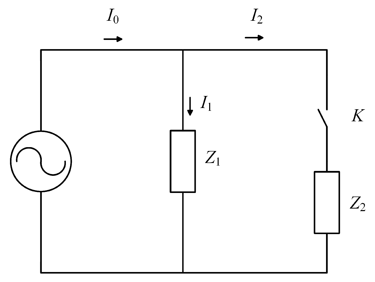
Originally, the inspiration about this paper comes from the parallel circuit shown in Figure 1. Assume that the main circuit current is $I_0$, and the branch currents are $I_1$ and $I_2$ respectively, and the background load and the target load are $Z_1$ and $Z_2$ respectively. When the switch K is turned off, we have the equation $I_{0\left(off\right)}=I_{1\left(off\right)}$, and $I_{0\left(off\right)}$ is known. After the switch K is turned on, we have the equation $I_{0\left(on\right)}=I_{1\left(on\right)}+I_{2\left(on\right)}$ according to Kirchhoff’s current law (KCL), and $I_{0\left(on\right)}$ is known. In the ideal case, it will be ignored that the effect of $Z_2$ on $Z_1$ and the fluctuation of $Z_1$ branch, thus $I_{1\left(off\right)}=I_{1\left(on\right)}$, further $I_{2\left(on\right)}$ can be expressed by:

$$\begin{array}{cc}\hfill I_{2\left(on\right)}& =I_{0\left(on\right)}-I_{1\left(on\right)}\hfill \\ & =I_{0\left(on\right)}-I_{1\left(off\right)}\hfill \\ & =I_{0\left(on\right)}-I_{0\left(off\right)}.\hfill \end{array}$$

(1)

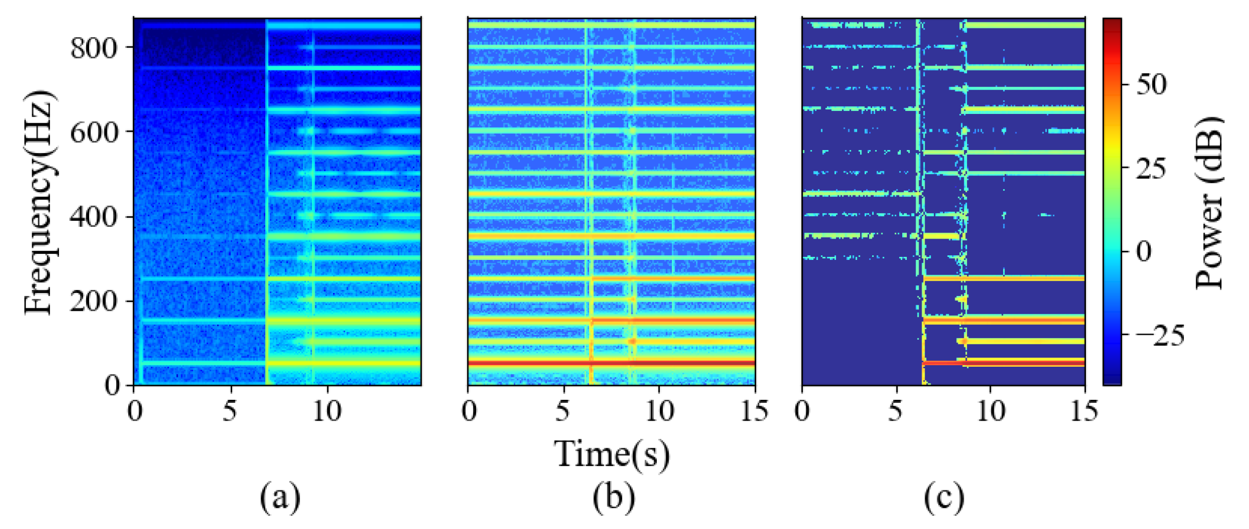
However, experiments shown in Figure 2 prove that Equation (1) does not strictly hold. Figure 2a shows the microwave spectrogram without background loads, which is measured in the laboratory. Figure 2b shows the microwave spectrogram in the UK-DALE dataset, Figure 2c shows the spectrogram calculated by spectral estimation based on the previous hypothesis of Equation (1). Although there is a strong correlation between Figure 2a and Figure 2c, spectral estimation does not eliminate the background load precisely, there are still intermittent spectral lines before the appliance is turned on. Besides, compared to Figure 2a, some detail components are eliminated in Figure 2c after the appliance is turned on. These phenomena prove that the background load has a certain degree of stationarity, but this does not mean it is exactly unchanged, and $I_{1\left(off\right)}$ is not equal to $I_{1\left(on\right)}$. Accordingly, the background load needs to be estimated more reasonably.

On this issue, this paper proposes a novel approach, concatenate deep neural network, to estimate the features of $I_{2\left(on\right)}$ indirectly, which can be represented as:

$$\begin{array}{cc}\hfill X_{2\left(on\right)}& =d_{\varphi }(X_{0\left(on\right)},X_{1\left(on\right)})\hfill \\ & =d_{\varphi }(X_{0\left(on\right)},s_{\phi }(X_{0\left(off\right)},X_{0\left(on\right)})),\hfill \end{array}$$

(2)

where $s_{\phi }$ is the function to extract the similar part of two features $\{X_{0\left(off\right)},X_{0\left(on\right)}\}$, $d_{\varphi }$ is the function to extract the different part of two features $\{X_{0\left(on\right)},X_{1\left(on\right)}\}$, X with different subscripts are features of spectrograms computed by the corresponding current, which can be calculated by:

$$X=f_{\theta }\left(SI\right)$$

(3)

where $SI$ is the spectrogram. The function $f_{\theta }$ is used to extract the features of the mixed load spectrogram and the background spectrogram.

The inspiration of function $s_{\phi }$ and $d_{\varphi }$ borrows from Code Division Multiple Access (CDMA), which allows multiple users to transmit independent information within the same bandwidth simultaneously, and the orthogonal spreading code is used to distinguish and extract signals from different users [31].

In the circuit model, the main circuit current $I_0\left(t\right)$ is given by:

$$I_0\left(t\right)=\sum _{k=1}^K{I}_k\left(t\right),$$

(4)

where K is the number of branches. The branch current $I_k\left(t\right)$ is expressed as:

$$I_k\left(t\right)=I_k^{rated}{c}_k\left(t\right)$$

(5)

where $I_k^{rated}$ is the rated current of the load on the k-th branch, which is a constant, and the $c_k\left(t\right)$ represents the time-varying noise function of the load.

Since appliances are relatively independent in construction and operation, their noise functions are almost uncorrelated with each other and can act as the spreading code in CDMA.

The i-th branch current is recovered by multiplying the noise function:

$$\begin{array}{cc}\hfill z_k\left(t\right)& ={\int }_{t_i}^{t_i+T}{I}_0\left(t\right)c_i\left(t\right)dt\hfill \\ & ={\int }_{t_i}^{t_i+T}\sum _{k=1}^K{I}_k\left(t\right)c_i\left(t\right)dt\hfill \\ & ={\int }_{t_i}^{t_i+T}\sum _{k=1}^K{I}_k^{rated}{c}_k\left(t\right)c_i\left(t\right)dt\hfill \end{array}$$

(6)

As the spreading code in CDMA is designed, the noise functions are assumed to be orthogonal in the ideal case, where

$${\int }_0^T{c}_k\left(t\right)c_i\left(t\right)dt=\left\{\begin{array}{cc}T,& \mathrm{for}i=k\\ 0,& \mathrm{for}i\ne k,\end{array}\right.$$

(7)

Therefore the branch current is restored as:

$$z_i\left(t\right)=I_i^{rated}T.$$

(8)

Unfortunately, unlike CDMA, it is difficult to get the precise “spreading code” for each appliance in practice, and background loads usually consist of multiple loads. Therefore the method of network fitting is used to recover branch current. The first step is to extract the spreading code, and the second step is to reconstruct the feature of the branch current. Then the simplified form of Equation (4) is:

$$\begin{array}{cc}\hfill I_0\left(t\right)& =I_B\left(t\right)+I_L\left(t\right)\hfill \\ & =I_B^{rated}{c}_B\left(t\right)+I_L^{rated}{c}_L\left(t\right),\hfill \end{array}$$

(9)

where $I_B$ and $I_L$ represent the branch current of background loads and the load to be recognized (i.e., target load), respectively. $c_B\left(t\right)$ and $c_L\left(t\right)$ are weakly correlated. In practice, it is easy to get the previous background loads $I_{B^{\prime }}\left(t\right)$ before the target load is turned on. On the hypothesis that background loads are stationary in a short time, the relationship between the noise functions $c_{B^{\prime }}\left(t\right)$, $c_B\left(t\right)$ and $c_L\left(t\right)$ is stated as:

$${\int }_0^T{c}_i\left(t\right)c_{B^{\prime }}\left(t\right)dt\approx \left\{\begin{array}{cc}T,& \mathrm{for}i=B\\ 0,& \mathrm{for}i=L\end{array}\right.,$$

(10)

In fact, such estimation is not rigorous, because stationarity does not mean complete equality, and weak correlation does not mean strict independence. Thus the similarity learning module $s_{\phi }$ is equiped to fit Equation (10), and the feature of background loads is obtained by:

$$feature\left(I_B\left(t\right)\right)=s_{\phi }\left(I_0\left(t\right),I_{B^{\prime }}\left(t\right)\right).$$

(11)

For the branch current, $I_L\left(t\right)$ can be calculated by subtraction through Equation (9). For the corresponding feature, the difference learning module $d_{\varphi }$ is used to fit the subtraction operation and obtain the feature of $I_L\left(t\right)$ by:

$$feature\left(I_L\left(t\right)\right)=d_{\varphi }\left(feature\left(I_0\left(t\right)\right),feature\left(I_B\left(t\right)\right)\right).$$

(12)

In summary, the model consists of an embedding module, a similarity learning module, a difference learning module and a classifier, which realizes the complete process of feature extraction, feature selection, and classification.

3.2. Model Architecture

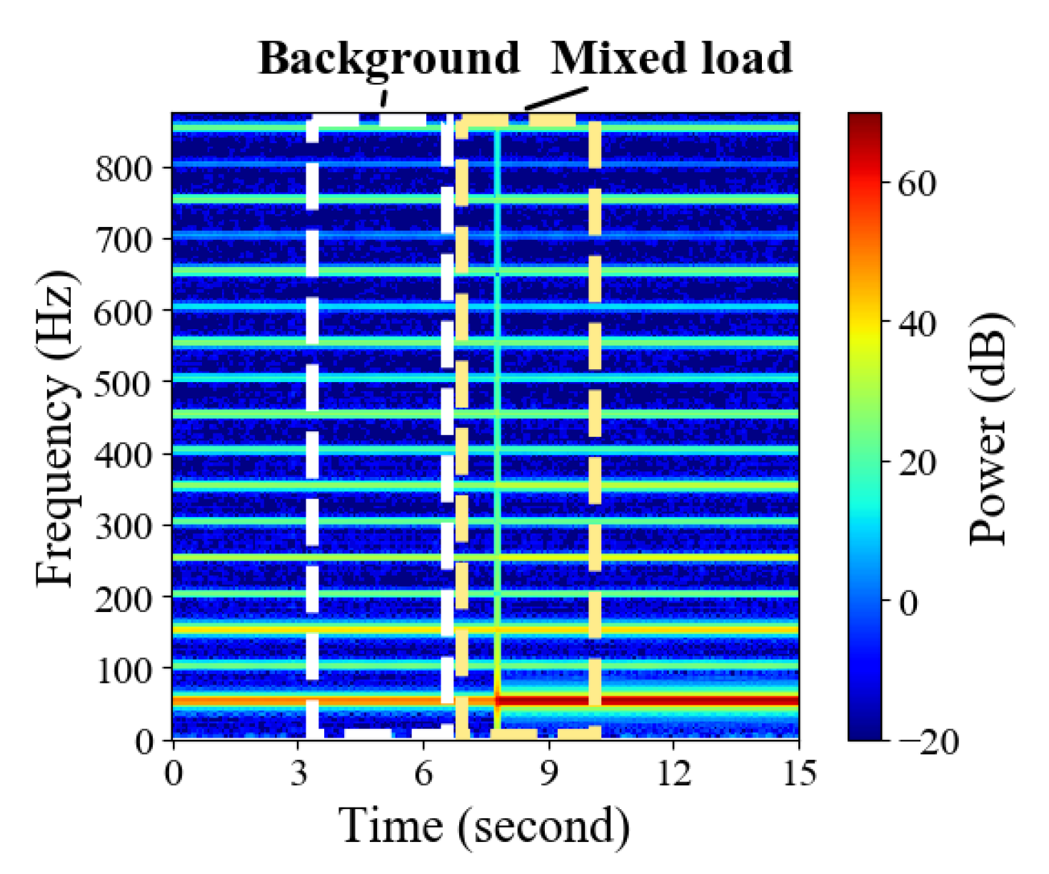
Based on the previous hypothesis, each spectrogram image is split into two blocks representing the background load and the mixed load as shown in Figure 3. Two blocks are input into the network simultaneously, which can be seen in Figure 4.

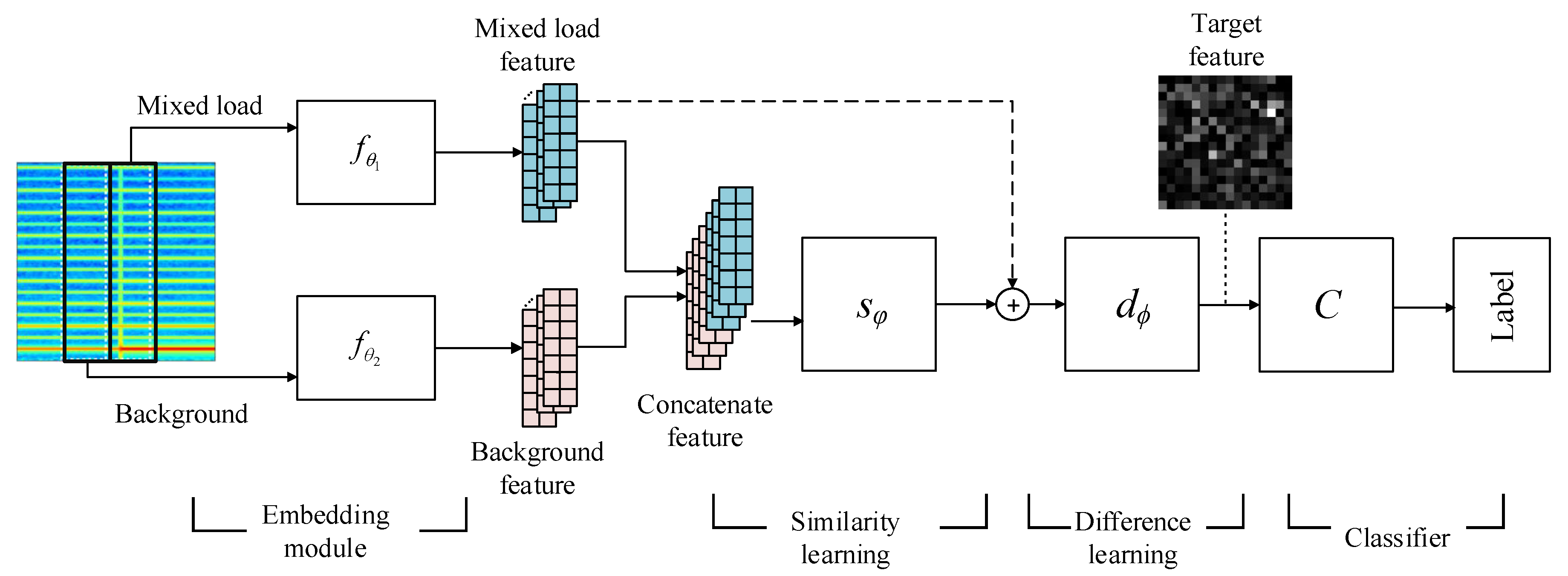
The CNNs in the embedding module are placed at the front end of the network to convert the image matrix into a vector, which is $f_{\theta }$ in Equation (3), and here the module comprises two networks $\{f_{{\theta }_1},f_{{\theta }_2}\}$ with the same structure and different parameters. The similarity learning module $s_{\phi }$ is used to generate the similar part in the concatenate feature and get the background feature behind the mixed feature, we refer to this as the “implicit background”, distinct from the “explicit background” extracted from the background-only load. The concatenation is channel-wise. The difference learning module $d_{\varphi }$ converts the features of the mixed load and the “implicit background” to the target feature $X_{2\left(on\right)}$. The final classifier determines the label of the target load through the target feature maps. The loss function is the cross-entropy function:

$$L=-\left(\sum _{i=1}^C{y}_i\log Z_i+(1-y_i)\log (1-Z_i)\right),$$

(13)

where $y_i$ is the i-th bit of the one-hot label y of C classes, and $Z_i$ is the i-th element of the network output Z with the softmax activation, which can be represented as:

$$Z=\mathrm{softmax}\left(h_{\sigma }\left(X_{2\left(on\right)}\right)\right),$$

(14)

where $h_{\sigma }$ is the classifier to map the obtained target spectrogram feature to the C-dimensional vector, and softmax is the activation.

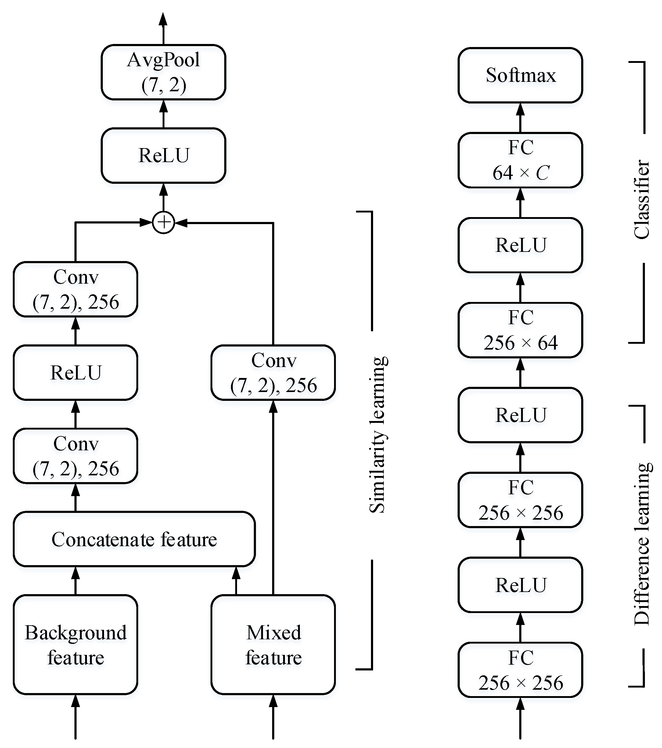
Figure 5 presents the detail architecture of the proposed network with the embedding module omitted. Similarity learning module seems to be a residual block even though it is not identical. The shortcut connection here aims to convey information about the mixed feature. Each convolutional layer (Conv) comprises a 256-filter convolution of kernel size $7\times 2$ and stride 1. The kernel size is determined by the embedding vector computed by the CNN. In all experiments, the size of the embedding vector (the background feature and the mixed feature) is $7\times 2\times 256$. The similarity learning module is followed by an average-pooling layer (AvgPool) with kernel size $7\times 2$ to compress the feature map in height and width. The output size of two fully connected (FC) layers in the difference learning module is 256. For the classifier, two FC layers are 64 and C dimensional, respectively.

4. Experiments and Discussion

The proposed approach is compared with two baselines and evaluated on the UK-DALE dataset and the BLUED dataset to test its universality. An energy disaggregation result on the UK-DALE dataset will be also provided.

4.1. Dataset and Data Preprocessing

Both the real and imaginary part of spectrograms are taken as model input, in other words, complex spectrograms are computed instead of power spectrograms or magnitude spectrograms. The two-channel data is more expressive not only because it contains phase information, but also due to the additivity of spectrograms in the complex domain. As envisaged, the background load can be removed from the mixed load on this account.

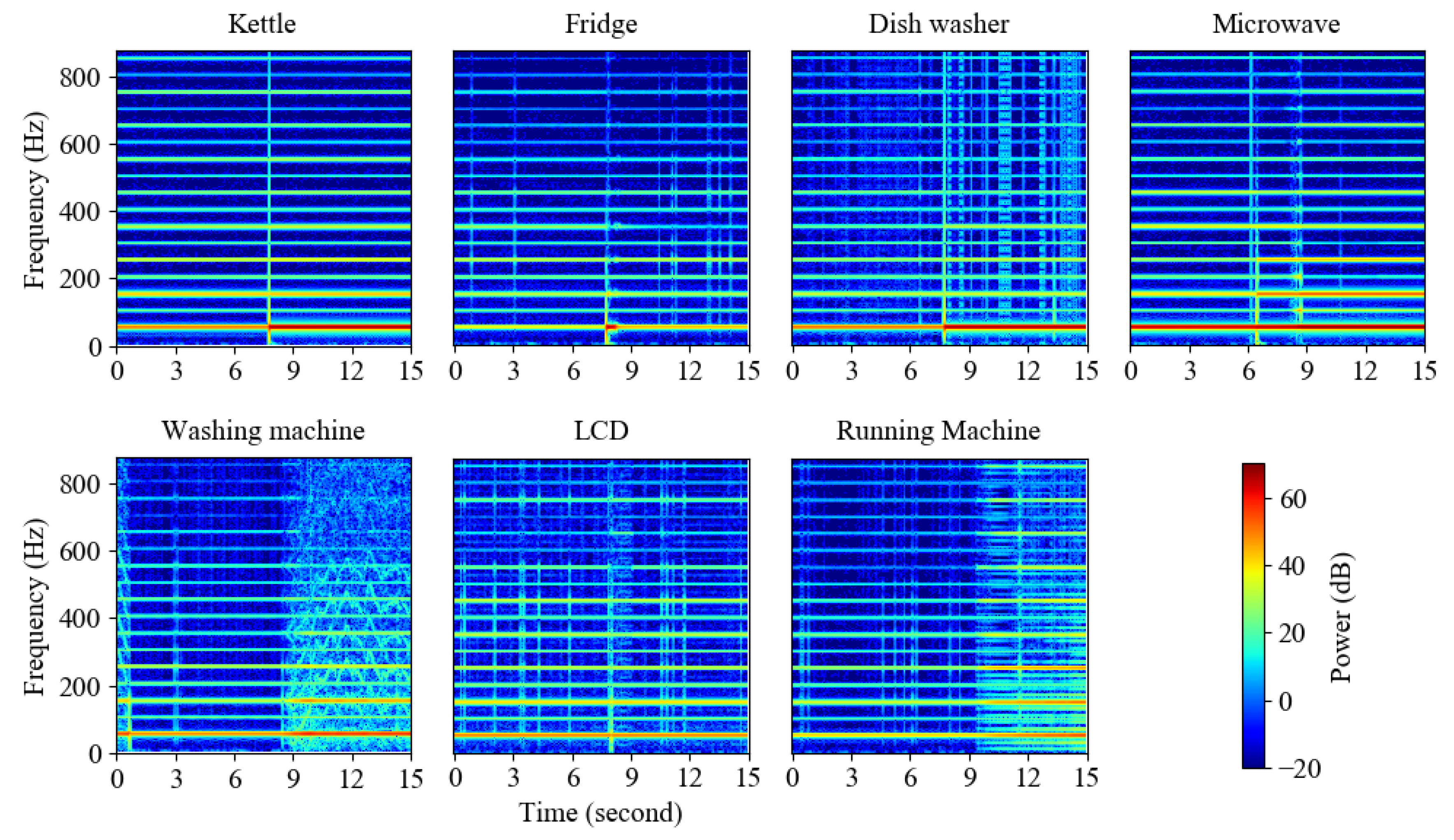
Every switching event contains 7-second current data, that is, 14,000 data points. As shown in Figure 6, plenty of samples are drawn to confirm that background loads are stationary in a 7-second window in most cases. Note that 15-second spectrograms are drawn in this paper in order to give a more complete demonstration, but this does not affect the 7-second spectrograms actually used in experiments. The size of an original 7-second spectrogram is $224\times 100\times 2$, the first two dimensions represent frequency and time, and the last dimension represents real and imaginary part. The switching point of each sample is located slightly after the midpoint of the time axis. As shown in Figure 3, two blocks are split from the original image as the proposed network input, and the splitting line is in the midpoint of the time axis. Every block of input image has a size of $224\times 50\times 2$.

4.1.1. UK-DALE

Most of our experiments are based on the UK-DALE dataset. The UK-DALE dataset contains electrical data from 5 houses for up to 655 days. A 1/6 Hz aggregate (mains) and individual appliance (submetered) power data were recorded for each house. Houses 1, 2, and 5 are selected as our original data source because only these 3 houses contain 16 kHz aggregate voltage and current data, then 16 kHz data is downsampled to 2 kHz to draw spectrograms. For submetered data, dataset authors did not record 16 kHz data. The switching events are detected with the help of submetered data (6-second time interval). For all experiments on UK-DALE, house 1 and house 5 data are set as the training set, and house 2 data is set as the test set to measure the generalization ability of our model. Seven classes of appliances are used for classification—kettle, fridge, dish washer (DW), microwave (MW), washing machine (WM), laptop or monitor (LCD), and running machine (RM). The number of appliances in each house and appliance spectrograms are shown in

Table 1. The number of appliance events per house in UK Domestic Appliance-Level Electricity dataset (UK-DALE).

Appliance	House 1	House 2	House 5
Kettle	4430	508	171
Fridge	7525	2172	2453
DW	2797	163	235
MW	536	299	29
WM	12311	785	521
LCD	4022	862	387

and Figure 6, respectively.

4.1.2. BLUED

Unlike the UK-DALE dataset, the BLUED dataset collects data from a house for only 8 days, which also has dozens of appliances, so each appliance has very few samples.

Table 2. Appliances used in Building-Level fUlly labeled dataset for Electricity Disaggregation (BLUED).

Appliance	Label	#Events
Fridge	Phase A, 1	282
Lights1 (backyard lights, washroom light, bedroom lights)	Phase A, 2	17
High-Power1 (Hair dryer, air compressor, kitchen aid chopper)	Phase A, 3	18
Lights2 (desktop lamp, basement light, closet lights)	Phase B, 1	38
High-Power2 (printer, iron, garage door)	Phase B, 2	52
Computer and monitor (computer, LCD monitor, DVR)	Phase B, 3	130

shows the selected appliances to facilitate comparison with the published work based on Fast Shapelets [32]. Raw data (12 kHz) is also downsampled to 2 kHz to draw the same size spectrogram as the one in the UK-DALE dataset. The validation set accounts for 33% and a 3-fold cross-validation is adopted.

4.2. Experimental Infrastructure

All neural networks in classification tasks are implemented using TensorFlow and trained on NVIDIA GeForce GTX 1080 GPUs.

In this paper, all networks are trained using Adam optimizer [33], and the initial learning rate is set to 0.001 for all networks, although some exceptions will be supplemented later.

4.3. The Recognition Result on UK-DALE

Two different prevalent networks are chosen as the embedding module of the model: Xception and DenseNet-121. We name these models Concatenate-CNNs. Meanwhile, two baselines are used to compare with the proposed networks. The model input and description is shown in

Table 3. Model input and description.

Model	Model Input	Model Description
CNN (baseline 1)	One $224\times 100\times 2$ original spectrogram	CNN with a FC classifier
CNN-SE (baseline 2)	One $224\times 100\times 2$ original spectrogram subtracts the estimated background	CNN with a FC classifier
Concatenate-CNN	Two $224\times 50\times 2$ spectrograms split from the original spectrograms	CNN with a similarity learning module, a difference learning module and a FC classifier

.

The first baseline is to classify appliances without the disposal of background loads. The original $224\times 100\times 2$ spectrogram is input into the CNN without concatenate features and following networks.

The second baseline is to deal with the background load with spectral estimation (SE). The model input is the estimated target spectrogram which is shown in Figure 2c, the network is the same as the first baseline, and we call this CNN-SE. In this case, the background current is assumed to be invariant during the window. Specifically, the background feature is obtained by calculating the average spectrum of the first 3 seconds in the entire 7-second window, the target spectrogram is obtained by subtraction between the original spectrogram and the calculated background spectrogram.

In Concatenate-DenseNet-121 and its two baselines, the growth rate is set to 32 and the compression rate is 0.5. Other parameters have been illustrated in the last section.

Here are three metrics to evaluate the performance. ’Recall’ indicates the proportion of samples of one class are correctly recognized, which is given by:

$$recall=\frac{TP}{TP+FN}.$$

(15)

’Precision’ represents the proportion of samples recognized as one class and truly belong to that class, which is calculated by:

$$precision=\frac{TP}{TP+FP}.$$

(16)

where true positives (TP) are the number of events correctly classified when the appliance was on, false positives (FP) are the number of events classified as on being the appliance off, and false negatives (FN) represent the number of events classified as off being the appliance on.

The F1-score combines recall and precision, here appliance events are classified without estimating the power consumption, thus the F1-score is reported [34], which is given by:

$$F1-score=2·\frac{precision·recall}{precision+recall}.$$

(17)

The performance of these models on the UK-DALE dataset is reported in

Table 4. Comparison of the proposed model and two baselines on house 2 data of the UK-DALE dataset with recall (%), precision (%), and F1-score (%). Best results are shown in bold.

Model	Metrics	Kettle	Fridge	DW	MW	WM	LCD	RM	Average
Xception	Recall	91.3	98.1	79.1	98.7	96.9	63.5	42.9	81.5
	Precision	91.7	99.9	39.1	98.3	77.6	99.5	81.8	84.0
	F1-score	91.5	99.0	52.3	98.5	86.2	77.5	56.3	80.2
Xception-SE	Recall	97.6	93.9	77.3	98.7	96.3	87.6	33.3	83.5
	Precision	93.0	99.0	35.9	98.7	95.6	98.3	87.5	86.8
	F1-score	95.3	96.4	49.0	98.7	95.9	92.6	48.3	82.3
Concatenate-Xception	Recall	99.6	99.6	84.7	96.7	98.9	71.9	52.4	86.2
	Precision	95.3	99.5	40.7	99.7	93.0	98.4	91.7	88.3
	F1-score	97.4	99.6	55.0	98.1	95.9	83.1	66.7	85.1
DenseNet-121	Recall	100	99.8	71.8	99.7	95.5	81.2	71.4	88.5
	Precision	91.4	99.6	66.9	98.7	85.7	99.4	71.4	87.6
	F1-score	95.5	99.7	69.2	99.2	90.3	89.4	71.4	87.8
DenseNet-121-SE	Recall	99.2	86.4	87.7	99.0	97.8	74.2	71.4	88.0
	Precision	95.6	99.9	22.3	99.7	95.5	99.5	78.9	84.5
	F1-score	97.4	92.7	35.6	99.3	96.7	85.0	75.0	83.1
Concatenate-DenseNet-121	Recall	100	99.6	77.9	99.3	92.4	93.0	57.1	88.5
	Precision	92.5	99.2	62.6	100	95.9	98.9	85.7	90.7
	F1-score	96.1	99.4	69.4	99.7	94.1	95.9	68.6	89.0

. The performance of concatenate models is highly depended on the embedding module, and concatenate structure improves the classification result on this basis. For two different CNNs as embedding layers, Concatenate-CNN models perform better than two baselines in average F1-score, as well as recall and precision for most appliances. The proposed model can achieve an equilibrium result among appliances in F1-score. However, the second baseline (spectral estimation) is just slightly better than the first baseline in Xception-SE, and DenseNet-121-SE is even worse than DenseNet-121. Accordingly, Concatenate-CNN models can eliminate background loads better, and the results make clear that background loads are not exact stationary. It is not rigorous to estimate the target spectrogram by directly subtracting the background spectrogram (baseline 2).

In

Table 5. F1-score (%) on house 2 data of the UK-DALE dataset. Fully connected (FC) output size/Conv filter size and Conv kernel size are tuned in Concatenate-DenseNet-121.

No.	FC Output Size/Conv Filter Size	Conv Kernel Size	F1-score
1	128	(7,2)	88.1
2	256	(7,2)	89.0
3	512	(7,2)	88.5
4	1024	(7,2)	89.5
5	256	(3,2)	87.1
6	256	(5,2)	88.1

, six options of network parameters in the similarity learning module and the difference learning module are compared. Small differences among models 1/2/3/4 prove that the proposed model is insensitive to FC output size/Conv filter size. Model 4 is marginally better than model 2, but the huge parameters increase model complexity and inference time. Model 2 is slightly better than model 6 and significantly better than model 5, which indicates that Conv kernel size has an observable effect on the model. To sum up, model 2 is selected for the rest of this paper.

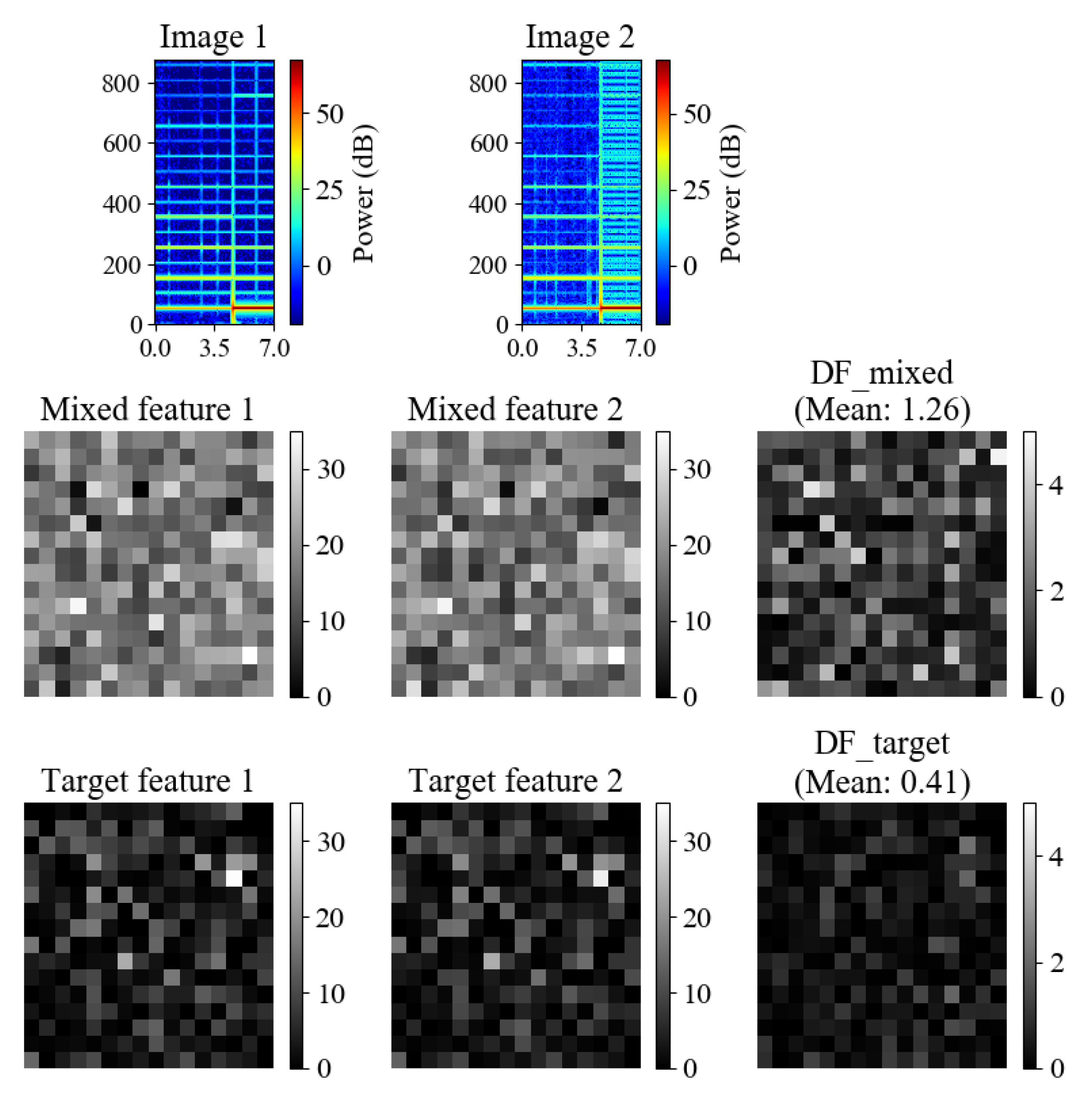
To further visualize the effectiveness of the model, the network’s response to two same class samples at different layers is shown in Figure 7, and the mixed feature and the target feature have been indicated in Figure 4. The shown mixed feature is averaged in height and width, retaining channel data. The difference of features is obtained by calculating the absolute value of the difference between the two columns on the left. Within a class, the target feature is more similar than the mixed feature, that is to say, the difference of target features (DF_target) is smaller than the difference of mixed load features (DF_mixed).

4.4. The Recognition Result on BLUED

The BLUED dataset contains many types of appliances with few samples, thus the model parameters of Concatenate-DenseNet-121 on UK-DALE are retained and applied to the BLUED dataset to avoid overfitting, then the BLUED data is trained for 30 epochs at a small learning rate of 0.0001.

The result of classification on the BLUED dataset is shown in

Table 6. The performance of classification on the BLUED dataset.

Label	Recall	Precision	F1-score
A1	98.8	95.5	97.1
A2	50.0	91.7	64.4
A3	71.4	94.4	81.2
B1	82.1	84.2	83.1
B2	94.1	98.0	96.0
B3	87.5	76.4	81.6
Average	80.7	90.0	83.9
Fast Shapelets [32]	77.6	69.7	72.3

. The Concatenate-DenseNet- 121 distinguishes 6 classes of appliances, whereas the Fast Shapelets algorithm [32] trains a single classifier on each phase, which only needs to distinguish 3 classes at a time. Nevertheless, the proposed approach improves recall by 3.5%, precision by 19.1%, and F1-score by 11.8%. The result on the BLUED dataset shows the validity of the model on small samples.

4.5. The Energy Disaggregation Result on UK-DALE

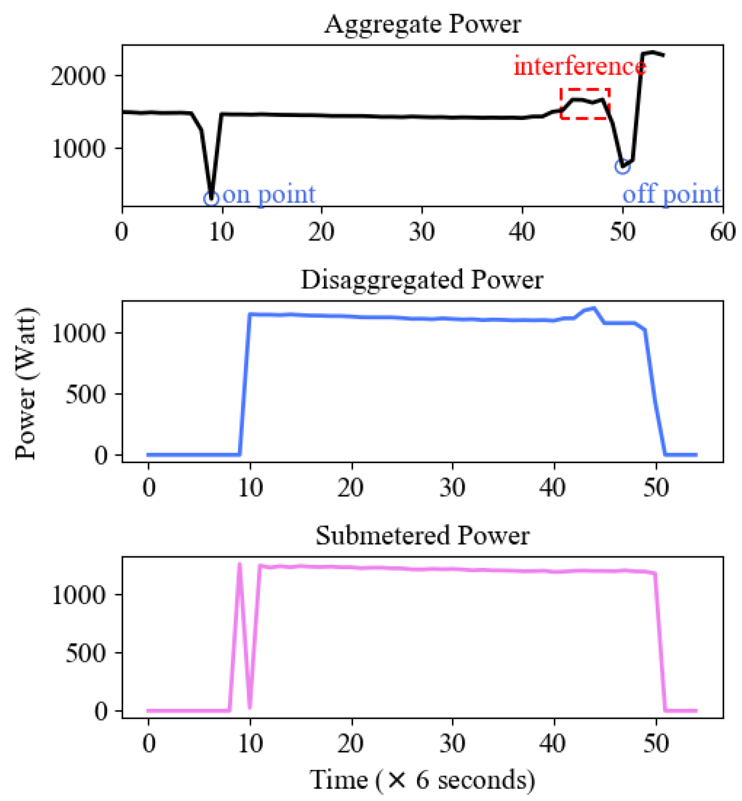
The main goal of this paper is to recognize the type of appliances, and energy disaggregation is considered a by-product. Switching events recognized by the previous appliance recognition algorithm determine where the appliance cycle is located, thus the appliance recognition results have a great impact on energy disaggregation. On-events are recognized by the Concatenate-DenseNet-121 network, then off-events are recognized through the power of previous on-events. After determining on/off time, the disaggregated active power data is derived from the translation and smoothing of the aggregate data. The entire process of energy disaggregation is summarized in Algorithm 1 and Figure 8 is an example of energy disaggregation.

Algorithm 1 Work Flow of Energy Disaggregation

Require: The aggregate power data at time t, $P_A\left(t\right)$    The on-events recognized by the classification task, $E_{on}=\left\{E_{on}\left(1\right),\cdots ,E_{on}\left(n\right)\right\}$    The power of individual appliance l, $P_l$ 1: Set threshold $T_l$ for appliance l 2: Detect a falling edge e 3: ife matches the power of $E_{on}\left(k\right)\in E_{on}$ then 4:  Determine the appliance label l and on/off time $t_{on}/t_{off}$ of an operation cycle 5:  for $i=t_{on}$ to $t_{off}$ do 6:   $P_A\left(i\right)\leftarrow P_A\left(i\right)-P_A\left(t_{on}\right)$ # Translation 7:   if $|P_A\left(i\right)-P_l|>T_l$ then 8:    $P_A\left(i\right)\leftarrow P_l$ # Smoothing 9:   end if 10:  end for 11:  Delete $E_{on}\left(k\right)$ in $E_{on}$ 12: end if

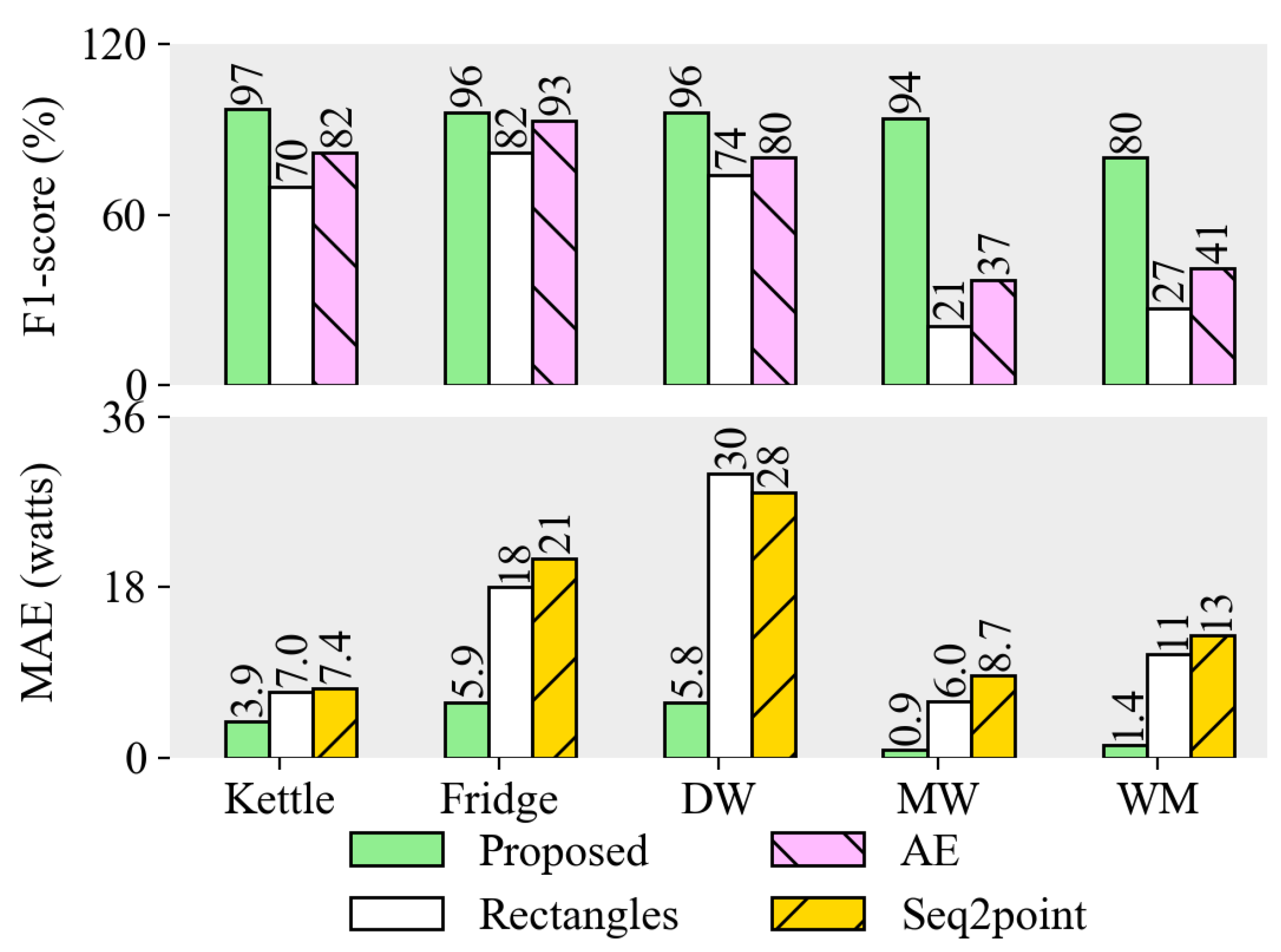
Five target appliances are selected for energy disaggregation except for LCD and RM in the classification task. The performance is presented on house 2 appliances with the training of house 1 and 5 data. True or false binary judgments no longer depend only on the classification of switching events, but whether each data point matches, thus the F1-score here takes power estimation into account, called the M-fscore in [34]. Mean absolute error (MAE) is introduced to measure the error in every single point [15]. Figure 9 shows the disaggregation result on house 2. The proposed model is compared with the best result in Kelly and Knottenbelt’s paper [15] in terms of F1-score and MAE, that is, the “Rectangles” architecture, and the performance is also compared with the result of AE [28] in F1-score and seq2point network [29] in MAE.

The energy disaggregation results of the recognition model outperform the network dedicated to energy disaggregation. With high disaggregation accuracy, concatenate CNNs can be used as an auxiliary tool for energy disaggregation. Compared with the other two methods, all the metrics are greatly improved, especially MAE is reduced in DW, MW, and WM.

The result proves that once the type of switching event is determined, the power waveform does not need a point-to-point reconstruction with neural networks or other approaches. The nuances in waveforms have a small effect, but the influence of incorrect appliance recognition is more critical. The events in the proposed approach are different from those in Kelly and Knottenbelt’s paper [15]. The event number of washing machine in this paper (Table 1) far exceeds theirs (less than 600). This is because multiple state transitions in each entire operation cycle are monitored in this paper. The location of every state transition greatly improves the result of energy disaggregation. Multi-state and programmable appliances will be a trend in the future, thus it is difficult to capture and train the entire operating cycle due to numerous combinations of states. It is worth mentioning that the approach in this paper recognizes appliances by high-frequency data, while the other methods in this section used low-frequency data. Obviously, high-frequency data is conducive to locating and distinguishing appliance events, and eliminating the influence of background loads facilitates energy disaggregation.

Table 7. The average execution time (AET) of the proposed model.

Model	AET (ms)
Concatenate-DenseNet-121 (CPU)	221
Concatenate-DenseNet-121 (GPU)	69

records the average execution time (AET) of the Concatenate-DenseNet-121 model. The CPU option means the model is executed with an Intel Core i3 processor and 8 GB RAM. The GPU option has been stated in Section 4.2. The AET consists of the inference time of the classification task and the running time of the disaggregation task. The AET of the proposed model is short enough to meet the requirement of continuous operation.

5. Conclusions

The concatenate convolutional neural networks proposed in this paper can apply favorably to appliance recognition and energy disaggregation. The proposed models are evaluated on two real world datasets: UK-DALE and BLUED. Experiment results show the capacity of the proposed model, which can partly resist the interference of the background load on both large and small samples. Besides, the approach presents great generalization ability in appliance recognition and energy disaggregation. The hypothesis of short time stationarity is a premise of the proposed model, which also restricts the window length of samples at the same time. However, there is still the exception that the transient-state process of some appliances is more than three seconds (e.g., running machine). Therefore, we intend to break through the restriction and estimate target features from the longer time mixed load in the future.

References

- Wytock, M.; Kolter, J.Z. Contextually Supervised Source Separation with Application to Energy Disaggregation. In Proceedings of the 28th AAAI Conference on Artificial Intelligence, Québec City, QC, Canada, 27–31 July 2014; pp. 486–492. [Google Scholar]
- Yu, L.; Li, H.; Feng, X.; Duan, J. Nonintrusive appliance load monitoring for smart homes: Recent advances and future issues. IEEE Instrum. Meas. Mag. 2016, 19, 56–62. [Google Scholar] [CrossRef]
- Siano, P. Demand response and smart grids—A survey. Renew. Sustain. Energy Rev. 2014, 30, 461–478. [Google Scholar] [CrossRef]
- Ephrat, A.; Mosseri, I.; Lang, O.; Dekel, T.; Wilson, K.; Hassidim, A.; Freeman, W.T.; Rubinstein, M. Looking to listen at the cocktail party: A speaker-independent audio-visual model for speech separation. ACM Trans. Graph. 2018, 37, 112. [Google Scholar] [CrossRef]
- Mogami, S.; Sumino, H.; Kitamura, D.; Takamune, N.; Takamichi, S.; Saruwatari, H.; Ono, N. Independent Deeply Learned Matrix Analysis for Multichannel Audio Source Separation. In Proceedings of the IEEE 26th European Signal Processing Conference (EUSIPCO), Rome, Italy, 3–7 September 2018; pp. 1557–1561. [Google Scholar]
- Chollet, F. Xception: Deep learning with depthwise separable convolutions. In Proceedings of the IEEE Conference on Computer Vision and Pattern Recognition (CVPR), Honolulu, HA, USA, 22–25 July 2017; pp. 1251–1258. [Google Scholar]
- He, K.; Zhang, X.; Ren, S.; Sun, J. Deep residual learning for image recognition. In Proceedings of the IEEE Conference on Computer Vision and Pattern Recognition (CVPR), Las Vegas, NV, USA, 27–30 June 2016; pp. 770–778. [Google Scholar]
- Huang, G.; Liu, Z.; Van Der Maaten, L.; Weinberger, K.Q. Densely connected convolutional networks. In Proceedings of the IEEE Conference on Computer Vision and Pattern Recognition (CVPR), Honolulu, HA, USA, 22–25 July 2017; pp. 2261–2269. [Google Scholar]
- Kelly, J.; Knottenbelt, W. The UK-DALE dataset domestic appliance-level electricity demand and whole-house demand from five UK homes. Sci. Data 2015, 2, 150007. [Google Scholar] [CrossRef] [PubMed]
- Anderson, K.; Ocneanu, A.; Benitez, D.; Carlson, D.; Rowe, A.; Berges, M. BLUED: A fully labeled public dataset for event-based non-intrusive load monitoring research. In Proceedings of the 2nd KDD Workshop on Data Mining Applications in Sustainability (SustKDD), Beijing, China, 12–16 August 2012; pp. 12–16. [Google Scholar]
- Hart, G.W. Nonintrusive appliance load monitoring. Proc. IEEE 1992, 80, 1870–1891. [Google Scholar] [CrossRef]
- Carli, R.; Dotoli, M. Energy scheduling of a smart home under nonlinear pricing. In Proceedings of the 53rd IEEE Conference on Decision and Control, Los Angeles, CA, USA, 15–17 December 2014; pp. 5648–5653. [Google Scholar]
- Sperstad, I.B.; Korpås, M. Energy Storage Scheduling in Distribution Systems Considering Wind and Photovoltaic Generation Uncertainties. Energies 2019, 12, 1231. [Google Scholar] [CrossRef]
- Hosseini, S.M.; Carli, R.; Dotoli, M. Model Predictive Control for Real-Time Residential Energy Scheduling under Uncertainties. In Proceedings of the 2018 IEEE International Conference on Systems, Man, and Cybernetics (SMC), Miyazaki, Japan, 7–10 October 2018; pp. 1386–1391. [Google Scholar]
- Kelly, J.; Knottenbelt, W. Neural NILM: Deep neural networks applied to energy disaggregation. In Proceedings of the 2nd ACM International Conference on Embedded Systems for Energy-Efficient Built Environments, Seoul, South Korea, 4–5 November 2015; pp. 55–64. [Google Scholar]
- Parson, O.; Ghosh, S.; Weal, M.; Rogers, A. Non-intrusive load monitoring using prior models of general appliance types. In Proceedings of the 26th AAAI Conference on Artificial Intelligence, Toronto, ON, Canada, 22–26 July 2012; pp. 356–362. [Google Scholar]
- Chang, H.H.; Chen, K.L.; Tsai, Y.P.; Lee, W.J. A new measurement method for power signatures of nonintrusive demand monitoring and load identification. IEEE Trans. Ind. Appl. 2012, 48, 764–771. [Google Scholar] [CrossRef]
- Froehlich, J.; Larson, E.; Gupta, S.; Cohn, G.; Reynolds, M.; Patel, S. Disaggregated end-use energy sensing for the smart grid. IEEE Pervasive Comput. 2011, 10, 28–39. [Google Scholar] [CrossRef]
- Kahl, M.; Haq, A.U.; Kriechbaumer, T.; Jacobsen, H.A. WHITED—A Worldwide Household and Industry Transient Energy Data Set. In Proceedings of the 3rd International Workshop on Non-Intrusive Load Monitoring, Vancouver, BC, Canada, 14–15 May 2016. [Google Scholar]
- Chui, K.; Lytras, M.; Visvizi, A. Energy Sustainability in Smart Cities: Artificial intelligence, smart monitoring, and optimization of energy consumption. Energies 2018, 11, 2869. [Google Scholar] [CrossRef]
- Figueiredo, M.; De Almeida, A.; Ribeiro, B. Home electrical signal disaggregation for non-intrusive load monitoring (NILM) systems. Neurocomputing 2012, 96, 66–73. [Google Scholar] [CrossRef]
- Le, T.T.H.; Kim, H. Non-Intrusive Load Monitoring Based on Novel Transient Signal in Household Appliances with Low Sampling Rate. Energies 2018, 11, 3409. [Google Scholar] [CrossRef]
- Gillis, J.M.; Morsi, W.G. Non-intrusive load monitoring using semi supervised machine learning and wavelet design. IEEE Trans. Smart Grid 2016, 8, 2648–2655. [Google Scholar] [CrossRef]
- Hassan, T.; Javed, F.; Arshad, N. An empirical investigation of V-I trajectory based load signatures for non-intrusive load monitoring. IEEE Trans. Smart Grid 2014, 5, 870–878. [Google Scholar] [CrossRef]
- He, K.; Stankovic, L.; Liao, J.; Stankovic, V. Non-intrusive load disaggregation using graph signal processing. IEEE Trans. Smart Grid 2018, 9, 1739–1747. [Google Scholar] [CrossRef]
- Makonin, S.; Popowich, F.; Bajić, I.V.; Gill, B.; Bartram, L. Exploiting HMM sparsity to perform online real-time nonintrusive load monitoring. IEEE Trans. Smart Grid 2016, 7, 2575–2585. [Google Scholar] [CrossRef]
- Cominola, A.; Giuliani, M.; Piga, D.; Castelletti, A.; Rizzoli, A.E. A hybrid signature-based iterative disaggregation algorithm for non-intrusive load monitoring. Appl. Energy 2017, 185, 331–344. [Google Scholar] [CrossRef]
- Barsim, K.S.; Yang, B. On the Feasibility of Generic Deep Disaggregation for Single-Load Extraction. In Proceedings of the 4th International Workshop on Non-Intrusive Load Monitoring, Austin, TX, USA, 7–8 March 2018; pp. 1–5. [Google Scholar]
- Zhang, C.; Zhong, M.; Wang, Z.; Goddard, N.; Sutton, C. Sequence-to-point learning with neural networks for non-intrusive load monitoring. In Proceedings of the 32nd AAAI Conference on Artificial Intelligence, New Orleans, LA, USA, 2–7 February 2018; pp. 2604–2611. [Google Scholar]
- Mocanu, E.; Nguyen, P.H.; Gibescu, M. Energy disaggregation for real-time building flexibility detection. In Proceedings of the 2016 IEEE Power and Energy Society General Meeting (PESGM), Boston, MA, USA, 17–21 July 2016; pp. 1–5. [Google Scholar]
- Hanzo, L.; Yang, L.L.; Kuan, E.L.; Yen, K. Single and Multi-Carrier DS-CDMA: Multi-User Detection Space-Time Spreading Synchronisation Networking and Standards; John Wiley & Sons: New York, NY, USA, 2003; pp. 35–80. [Google Scholar]
- Patri, O.P.; Panangadan, A.V.; Chelmis, C.; Prasanna, V.K. Extracting discriminative features for event-based electricity disaggregation. In Proceedings of the 2014 IEEE Conference on Technologies for Sustainability (SusTech), Ogden, UT, USA, 30 July 2014; pp. 232–238. [Google Scholar]
- Kinga, D.P.; Ba, J. Adam: A Method for Stochastic Optimization. In Proceedings of the 3rd International Conference for Learning Representations (ICLR), San Diego, CA, USA, 7–9 May 2015. [Google Scholar]
- Makonin, S.; Popowich, F. Efficient sparse matrix processing for nonintrusive load monitoring (NILM). Energy Efficien. 2014, 8, 809–814. [Google Scholar] [CrossRef]
Figure 1.
The parallel circuit.
Figure 2.
Spectrograms of microwave. (a) The spectrogram with no background load. (b) The spectrogram with background loads (c) The estimated spectrogram.
Figure 3.
The background load part and the mixed load part of a complete spectrogram.
Figure 4.
The structure of concatenate convolutional neural networks (CNNs). The concatenation operation is channel-wise.
Figure 5.
The detail architecture of similarity learning and difference learning module. The addition operation ⨁ in similarity learning module is element-wise.
Figure 6.
Spectrograms drawn from appliances in UK Domestic Appliance-Level Electricity dataset (UK-DALE).
Figure 7.
An example of the network Concatenate-DenseNet-121’s response at different layers. The model input is two kettle samples with different background loads. For each layer, the output is reshaped to form a 2D image.
Figure 8.
An example of energy disaggregation. The red dashed box stands for interference from other appliances. The blue circle stands for on/off points of an operation cycle.
Figure 9.
Energy disaggregation results on the UK-DALE dataset.