Oil Factor in Economic Development


1
Department of Economy and Management, Azerbaijan State University of Economics (UNEC), Istiqlaliyyat Str. 6, Baku AZ‒1001, Azerbaijan
2
Department of Regulation of the Economy, Azerbaijan State University of Economics (UNEC), Istiqlaliyyat Str. 6, Baku AZ‒1001, Azerbaijan
*
Author to whom correspondence should be addressed.
Energies 2019, 12(8), 1573; https://0-doi-org.brum.beds.ac.uk/10.3390/en12081573
Submission received: 25 March 2019
/
Revised: 14 April 2019
/
Accepted: 18 April 2019
/
Published: 25 April 2019
Abstract
:The research examines the role of oil in the world economy and the evaluation of the oil factor in the economy of Azerbaijan. The error correction model (ECM) has been used in terms of reliability of the obtained results, and assessment has been done by the FMOLS, DOLS and CCR co-integration methods. Engel-Granger and Phillips-Ouliaris co-integration tests have been used for checking the co-integration relations among variables. Times series have been checked whether they are unit root (Augmented Dickey-Fuller (ADF), Phillips-Perron (PP) and Kwiatkowski-Phillips-Schmidt-Shin (KPSS) as a methodology of the research. The results of the research reveal that daily oil production and consumption have less effect on the formation of the world oil prices. On the other hand, the impact of the world GDP and world industry production volume is a bit more. Generally, the influence of these factors on oil market has been reduced gradually. However, the reverse process is observed during the analysis of the influence of oil production and oil price on the main indicators of Azerbaijan and Kazakhstan. Therefore, Azerbaijan and Kazakhstan are an oil-exporting countries which is why their macroeconomic indicators, especially currency, GDP and DNP, heavily depends on the oil factor. The research has been limited but highlights the obtained results to some problems and this must be considered as a new source for future research. Thus, the similar studies have been considered to be done thoroughly on several alternative econometric models, but a lack of statistical information on a yearly basis and strong currency intervention constitute some barriers to transiting to a floating currency. The practical importance of the research is to prove that the dependency of the oil prices on the world GDP and world industry production, daily oil production and world oil consumption have decreased gradually. In the second part of the research, the dependency of the Azerbaijan and Kazakhstan economies on oil was proved. This might be a signal to transfer oil resources into human capital.
1. Introduction
Oil remains as main source of energy for the world. Numerous countries are the participants in this process. Currently, there are more than 100 oil-exporting countries in the world. Oil prices affect both oil-exporters and importers. The oil price affects the producers and the level of production expenditures. Some countries’ economy are highly reliant on oil and oil products. That is why research on oil and its role in the economy is very important.
Oil factors affect political and economic processes. In turn, these affect the price level, inflation, economic revival, finance and stock market and economic growth as a whole. Meanwhile, it affects the formation of alternative energy resources and the development of these resources.
However, these influences are reciprocal. Thus, some non‒oil factors affect oil production and the development of the oil sector as well as some non-oil factors. The level of oil price and its formation is determined by the demand and supply of fuel in the world market. It is divided into traditional and recent factors.
The traditional ones are as follows: a period (of restoration and downsizing) in the world economy; the magnitude of oil production and extravagant oil deposits; the geopolitical situation of the main oil exporting regions; information about the exhaustion of oil reserves in the planet; oil and oil reserves in oil importing countries and the level of reserves of oil exporting countries; the statements of OPEC members concerning production quotas and price targets; oil infrastructure and natural and technical calamities; seasonal meteorological conditions; constraints between supply and demand to oil quality; ecological problems, etc.
The recent ones are as follows: impossibility of regulation of the financial market, opening oil markets to financing and extreme speculation; the growth of oil demand in new market economies; the fluctuation of the euro to dollar exchange rate. These and similar factors have a special weight and influence on the terms of demand and supply in the physical and “paper” oil markets.
While analysing the oil market structure, it is important to pay attention to standard parameters of real commodity flow, demand change and the dynamics of oil production in the main exporting countries. However, oil-importing countries pay attention to the volume of strategic and commercial reserves. It has a long time that oil prices are not determined as it is now in the commodity market. Pricing is not carried out in the physical commodity market but in stock.
As a result of the development of derivative oil trading, a large amount of capital has penetrated into the market. This tendency has already turned it into a market with a high volatility from the classic financial market into currency and financial markets.
During the summit in Er‒Riad in 2007 November, the heads of state present mentioned that the current trend in the market that formulates the world oil market is not related to OPEC. The summit participants concluded that financial factors have a crucial role by analyzing the lack of production capacities in oil production, reduction in the world oil reserves, natural cataclysms, political events and processes, and financial factors. Oil has turned into a speculative object in the financial market rather than a real commodity. In this regard, the role of the oil factor in the economy has been investigated in terms of oil imports, oil production, economy of exporting countries, conjuncture of financial and stock markets and exchange rates.
After the 1990s, like other former Soviet Union republics, Azerbaijan and Khazakhistan declared their political independence. They were very strong partners of USSR in the world. Both of them embarked on producing and exporting hydrocarbon resources to the world market since they were now politically independent countries. That’s why their social and economic development, financial stability, GDP and other macroeconomic indicators became dependent on oil prices. However, these two countries made reforms in order to minimize the dependency and use resources effectively. Our research and analysis addresses the significance of this policy.
2. Literature Review
2.1. Oil and Economics
Researching energy production as a distinct factor began in economics when the world witnessed the first oil shock, in a sense, the oil market price increase in 1973. Since then economists have done a plethora of studies to assess the flexibility of production functions, especially energy and other factors [1,2,3,4]. Solow mentioned that flexibility was the key indicator to fathom the influence of price fluctuations on macroeconomics for the energy sector [5]. Kim and Loungani [6], Rotemberg and Woodford [7] and Finn [8] considered energy as a production factor in order to analyse the effectiveness of oil price changes. Carlstrom and Fuerst [9] and Leduc and Sill [10] analyzed price, money and credit policy during oil price shocks. However, most of these studies have been devoted to oil-importing countries.
Oil is different from other commodities for its features and lack of renewability. Some countries hope to importing oil because oil exporters are not many. Azerbaijan’s economy largely depends on factors that occur in the world oil market because it is also an oil exporter.
The development of economics as well as oil and gas infrastructure of oil-exporting countries has closely tied up with the prices of raw materials, either in external or internal marketx. Price fluctuations directly affect the market. It either increases or reduces competitiveness. Oil price dynamics might generate hesitations, especially in energy and oil crises. This has happened several times in countries where a market structure has developed.
A number of factors cause the increase in oil price: the growth rate of the world economy, price fluctuations in previous years, demand for raw materials, population (for example in Southeast Asia), hydrocarbon resources in different countries and regions, investment allocations of key players in the market and other factors. Reduction in oil price expands instability factors in the economy of exporter countries. It has already been revealed that the sharp increase in oil prices in 2000 was the result of military operations of the USA and Western countries in Iraq as well as political and military events in Northern Africa and Near East countries. On the other hand, ongoing demand for energy in Asian countries, especially China, had a great effect on the prices.
Ghalayini [11] researched the fluctuation of oil prices and concluded that price shocks affected macroeconomic indicators through different channels. Geopolitical doubts and certain market dissensions paved the way for mercenaries and speculative resources to affect the world oil market. In turn, this caused an increase of prices for a short period again [12]. Other economists like Hamilton [13] and Bruno and Sachs [14], who researched the fluctuation of oil prices, explained the impact of oil prices on economic development, instability of financial growth and inflation in 1950‒1979 in the UK. They came to a conclusion that the variables were closely connected to each other. Thus, fluctuations affects large economies unconstructively. The increase of oil price causes the increase of prices in the economy and reduces employment and productivity [15].
The influence of oil prices on macroeconomic indicators has been widely examined since Hamilton [13]. Hamilton [16] proved that the increase of oil price is more important than its fall. Hamilton used Sims’ [17] VAR method [18] to analyze the American economy during 1948‒1980 and concluded that oil prices and GDP growth in the USA were strongly correlated. Meantime, he also mentioned that oil price had been sharply changed until the recession period after World War II. Hamilton and other researchers (Gisser and Goodwin [19], Mork [20], Lee and others [21], Hamilton [22], Hamilton [23]) concluded that oil price had a negative influence on the GDP of the USA.
Some researchers noted that real oil prices were linear, but this rises the question of whether the influence of oil prices is really linear or not? Economists has been drawn by this problem. Mork [20] made a new proposal. He used information about the oil price fluctuations and pointed out that the oil price change had an asymmetric influence on the GDP of the USA. After Mork [20], Hamilton [22] proposed a non-linear method. He called it a quick method that responds to a non-linear modelling of oil prices. He named it “net growth of oil price” (NOPI). After Hamilton, Lee et al. [21] used GARCH model and indicated another non-linear oil-price function.
The asymmetric influence of oil price fluctuations on the economy was noted in the Andreopoulos [24], and Kilian and Vigfussion [25] studies. Structural models of the asymmetric effect on energy price fluctuation might not be assessed through the VAR method in their studies. They proposed an alternative structural regression of tests of symmetry to estimate models. They suggest a fundamental change is required in the methods to estimate the asymmetric effects of oil energy price shocks although this evidence is noted as complementary rather than a challenge by Hamilton [26].
What might the reasons of asymmetric effects of oil price fluctuation be? Is this the reason of currency policy or anything else? Hamilton [27] proposed that the reason for assymmetry might be the regulations of oil price changes. Ferderer [28] provided a number of explanations. According to his results, sector fluctuations and uncertainty in the economy might be linked with asymmetry but money and credit policy are not responsible for the asymmetry effect of oil price fluctuations. However, Bernanke et al. [29] concluded that the influence of oil crisis on the economy happens because of oil price changes. Currency policy is responsible for the asymmetry fluctuations of oil prices. They assume that currency policy might be used to minimize the results of recession periods. However, Hamilton and Herrera [30] criticised this statement. In a response to Hamilton and Herrera, Bernanke et al. [31] confirmed that the intensity of any external shock depends on the response of financial institutions to the same shock.
Raw material fluctuations are a common case for the global oil market. Thus, the world economy met a number of changes in raw material price in different periods. Oil price fluctuations are closely tied with historical events. For example, Hamilton [32] patterned a series of events that have affected oil prices such as the oil crisis after World War II, the Suez Cannel crisis in 1956–1957, the embargo on oil exports by OPEC in 1973–1974, the Iranian revolution in 1978–1979, the Iran–Iraq war in 1980, the Persian Gulf war in 1990–1991 and oil price increases in 2007–2008. Oil prices soared up to a historical record—140 US dollars per barrel—in 2008. This has been the highest price seen in the oil market [33].
Besides, it has been concluded that oil pricex interconnect with the legislation of local authorities [34]. The increase of oil prices causes inflation to go up and reducex the profitx generated from products and services and weakens economic development. Every government faces this problem when they want to increase oil prices [35]. Oil prices have a huge influence on the world economy but it is hard to determine because they are different for each country [36,37].
Besides, Katsuya [38] examined the effect of oil prices and credit fluctuations on real GDP and inflation in Russia in 1997–2007 and confirmed that the influence of money and credit fluctuations on economy is more powerful than that of oil fluctuations. However, this result is the opposite of what Hamilton and Herrera [30] determined.
Kilian [39] concluded that although external oil factors and fluctuations in 1970 influenced the economy significantly, the American economy was less affected by them, compared to other factors. Edelstein and Kilian [40] used the VAR method and gave evidence that the oil price influence is not as much as that of other factors.
Michael [41] has concluded that impact of energy resources on the economy is completely different from other resources. He claimed that inflation was directly influenced by oil prices. Besides, Turkish scholars Berument and Tasc [42], Aydo Agush [43], Olgun [44] researched the influence of oil prices on Turkey, inflation and economic development. They concluded that salary and other factors such as profit, interest rate and rent must be regulated on the basis of oil prices and the level of correct prices.
While talking about the demand and supply for fluctuating oil prices, China, the main oil importer, must be specifically noted. China also produces oil but its demand outweighs supply. That is why oil prices are expected to increase because of oil demand [45]. China occupies the second place for oil consumption and oil importing economy in terms of GDP. China is currently using all its power and resources in order to reach energy resources and foreign assets. It is assumed that China will have used more than half of world oil consumption by 2035. Lin and Chunping have done a thorough study of oil consumption in the transport sector in China’s economy. They have indicated a dependency among oil consumption, GDP, road conditions, productivity and oil prices [46]. Kilian [47] stated that rapid development of economic systems such as China’s have caused the increase of world oil demand and the surge in oil prices in 2008.
2.2. Oil Prices and the Stock Market
The stock market is one of the main indicators for market-oriented countries that is why, studying the mutual relations of these factors with oil prices is important. Nicholas and Miller [49] analysed mutual relations between share prices in developed countries (Australia, Canada, France, Germany, Italy, Japan, Great Britain, USA) and structural changes of oil market using a SVAR model.
They concluded that fluctuations in oil market didn’t affect much the stock market.
Basher and Sadorsky [50] researched the mutual relations between oil prices and emerging stock markets using the example of Brazil, Russia, India, China (BRIC) and the CAPM model. They concluded that the stock markets of Russia and Brazil were strong, while India and China witnessed the opposite. Aloui et al. [51] researched the impact of oil prices on the stock market of the developing countries (roughly 25 countries). They proved that oil prices are not strong enough to analyse the dependency and co-integration of data in 1997–2007. However, we have witnessed the opposite in the studies. They are asymmetric. Undoubtedly, dependency is positive for all countries, but it doesn’t have enough potential to determine the stock market on long term. Moreover, Kilian and Park [52] mentioned that the increase of oil price had a negative impact on the stock market.
Filis et al. [53] revealed a direct relationship between markets in Canada, Mexico, Brazil, USA, Germany, and The Netherlands from January 1987 to December 2009. They concluded that the dependency between developing countries in the crisis was in progress. Li et al. [54] researched mutual relations between oil price and the Chinese stock market using co-integration and casual analysis. Data were taken from July 2001 to October 2005 and from November 2005 to June 2007. It was determined that the dependency was direct.
In relatively stable periods, a bilateral interdependence between oil production and stock market indices is observed. We can’t consider it unexpected: demand for oil has declines in crisis periods. We can observe this in its production.
The researchers Rangan and Modise [55] stirred controversy by putting forth some ideas about the impact of oil price on the stock market (monthly indicators of 1997–2010) of the developing countries (on the example South Africa). The correlation has not been determined and its coefficient was low. Hammoudeh and Eleisa [56] researched the mutual dependency between the value of shares and oil price in five countries around the Persian Gulf (namely Bahrein, Kuwait, Oman, Saudi Arabia and United Arab Emirates). They concluded that there is a relationship between the value of shares and oil prices in the stock market of Saudi Arabia. Awartani and Maghyereh [57] researched the impact of world oil market on the stock markets in the Persian Gulf—Bahrein, Kuwait, Oman, Qatar, Saudi Arabia and the UAE (January 2004 and December 2011). They concluded that oil market largely depended on oil production in crisis periods by using analysis and a GARCH model. The volatility of the market increased in this period, but in relatively stable periods, its dependency on oil production is relative weak.
2.3. Oil Price and Exchange of Currency
Theoretically, oil price fluctuations influence on the currency of exporting countries in two directions:
In terms of trade—in the case oil prices soar, trade balances rocket, respectively, for oil exporting countries. By the time, their currency becomes expensive in the ratio of USD which is the currency of all contracts and purchases.
In the effect of wealth—while oil prices increase, wealth is transferred from oil importing countries to oil exporting countries. That’s why, their currency is getting expensive at the expense of international investors who create demand in the market by obtaining currency of oil exporting countries.
Keynes mentioned that the weakest point of Cassels’ “The Purchasing-Power-Parity Theory of Exchange Rates” was ignoring the changes in terms of trade. Not only does he refute the results of this theory, but also made it more fraudulent in the short term [58]. Gregorio and Wolf’s [59] research papers were just about the same issue. A plethora of researchers have examined the relations between oil price and exchange rates. Some researchers have indicated the cause and effect interrelations between price and exchange rates (Amano and Van Norden [60], Akram [61], Benasasy-Quere et al. [62], Lizardo and Mollick [63]). However, others proved the opposite: exchange rates affect oil prices (Brown and Phillips [64], Cooper [65], Yousefi and Wirjanto [66], Zhang et al. [67]). Some scientists give evidence that there are no relations between oil price and exchange rates.
Coudert et al. [68] calculated that long‒term flexibility of real exchange rates of currency for raw-material exporting countries on raw material prices was not so high. This flexibility is around 0.5 but for oil, it is around 0.3. Such cases are not observed in all raw-material exporting countries.
Cashin et al. [69], observed real prices on raw material and co-integration of real exchange rates only in 1/3 of 58 raw-material exporting countries in 1980–2002. They didn’t confirm that real prices of raw materials played an important role on exchange rates, but they succeeded in indicating that real prices are an important factor for raw-material exporting countries. Besides, Habib and Kalamova researched the exchange rates of Norway, Russia and Saudi Arabia and concluded that only the Russian rouble had an co-integration with oil prices in 1995–2006 [70].
Barsky and Kilian [71] concluded that the economic downsizing during the 70–80s of the XXth century was closely linked with the currency policy of the U.S. Federal Reserve System in order to eliminate the negative effects that the oil sector had created. Moreover, we have recently reseached Tony Klein’s article titled “Trends and Contagion in WTI and Brent Crude Oil Spot and Futures Markets during 2007–2017” [72].
Scientists-economists have applied a number of econometric models in order to research the influence of oil price on the world economy, stock market, oil exporting and importing countries’ economy and currency.
Buetzer et al. [73] did the largest empiric research work in 1986–2013 embracing 43 countries but couldn’t find any evidence proving a systematic revaluation of oil exporting country’s currencies after oil shocks. This partially relates to the fact that oil exporting countries actively increase foreign exchange rates in order to soften revaluation pressures on their currency. However, oil shocks are not important factors for the global configuration of exchange rates.
Many studies have highlighted that raw material prices are less exogenous toward exchange rates. For example, Chen and Rogoff researched how exogenous raw material prices were toward exchange rates of raw-material exporting countries such as Australia, Canada and New Zealand and concluded that price fluctuations penetrated into the exogenous shocks of trade terms. These shocks significantly affect to the main part of their exports. Thus, the world prices of raw material towards exchange rates are exogenous [74].
Nominal information is used in the calculations. Calculations have been implemented with the help of softwares like Gretl and EViews. They noted that the simple dependency coefficient is 0.084 by researching dependency between oil price and the rouble exchange rate (T = 835). The “null hypothesis” is rejected: t‒statistics = 2.436, bilateral p‒value = 0.015. This argument doesn’t support the opinions of Buetzer et al. [68] which the same as in the theory. Oil shocks are not important factors for the global configuration of oil shocks. However, the simple dependency coefficient increased by 0.962 in 9 June 2014–28 January 2015 (Т = 82). The “null hypothesis” is vehemently rejected. t = 45,723, р = 0. The main reasons why the rouble declined in March 2015 and June 2014 were revealed by this. It also refers to the Azerbaijani manat.
Buetzer et al. [75] noted that “rouble is not a norm, it is exception”. Oil prices have declined recently. Exchange rate markets must consider this. However, oil prices are not closely related to exchange rates, so oil price volatility was observed from an economic point of view. That is why, there are two factors which feature the tendency of oil changes in econometric models. Recently, there is an increasing tendency towards establishing mutual relationships between oil prices and the dollar. For example, Yousefi and Wirianto researched the fluctuation of cause and effect relations between OPEC tariffs and USD exchange rates using the Generalized Methods of Moments of Khansen in 2004 and proved that there was a negative dependency between them. Cifarelli and Paladino researched the mutual relationships of the USA oil price dynamics and the movement of exchange rates using a CCC GARCH‒M multi-variant model and revealed their mutual impact [76].
In 2004, Akram studied the non-linear interaction between the oil price and the exchange rates of some European countries (especially Norway) [61]. Further studies have also referred to the ratio between the oil prices and the exchange rates as well as the mutual impact between them. For example, Krichene used VECM and TGARCH models in order to confirm the impact of the nominal exchange rates in the example of the US on both increases and declines in oil prices in 2005 in the long and short-term period [77].
In 2010, Lizardo and Mollick used co-integration analysis to reveal the impact of oil prices on the dollar exchange rate in the long term. Thus, the increase in the real price of oil causes the reduction of the dollar in the oil exporting countries. These studies confirm that there is a contradiction between the oil price and the exchange rate [63]. The USA delineated the structure of interdependency between oil price and dollar in different times in the USA and Germany using the Bekiros and Dick Augmented Dickey-Fuller-ADF method [78]. By using a VAR (Chow test) model, Ramazan et al. [79] proved that oil price impacts the dollar weakly but stably in the long term, however, it has a more obvious impact in the short-term in the USA.
3. Data
In this research, world GDP, world industry production, daily oil production and including oil price have been generated using internet resources [www.ycharts.com]. Azerbaijan and Kazakhstan macroeconomic indicators have been taken from the Azerbaijan State Statistics Committee [www.stat.gov.az] and Kazakhstan State Statistics Committee [www.stat.gov.kz], respectively.
3.1. World Economy and Oil Prices
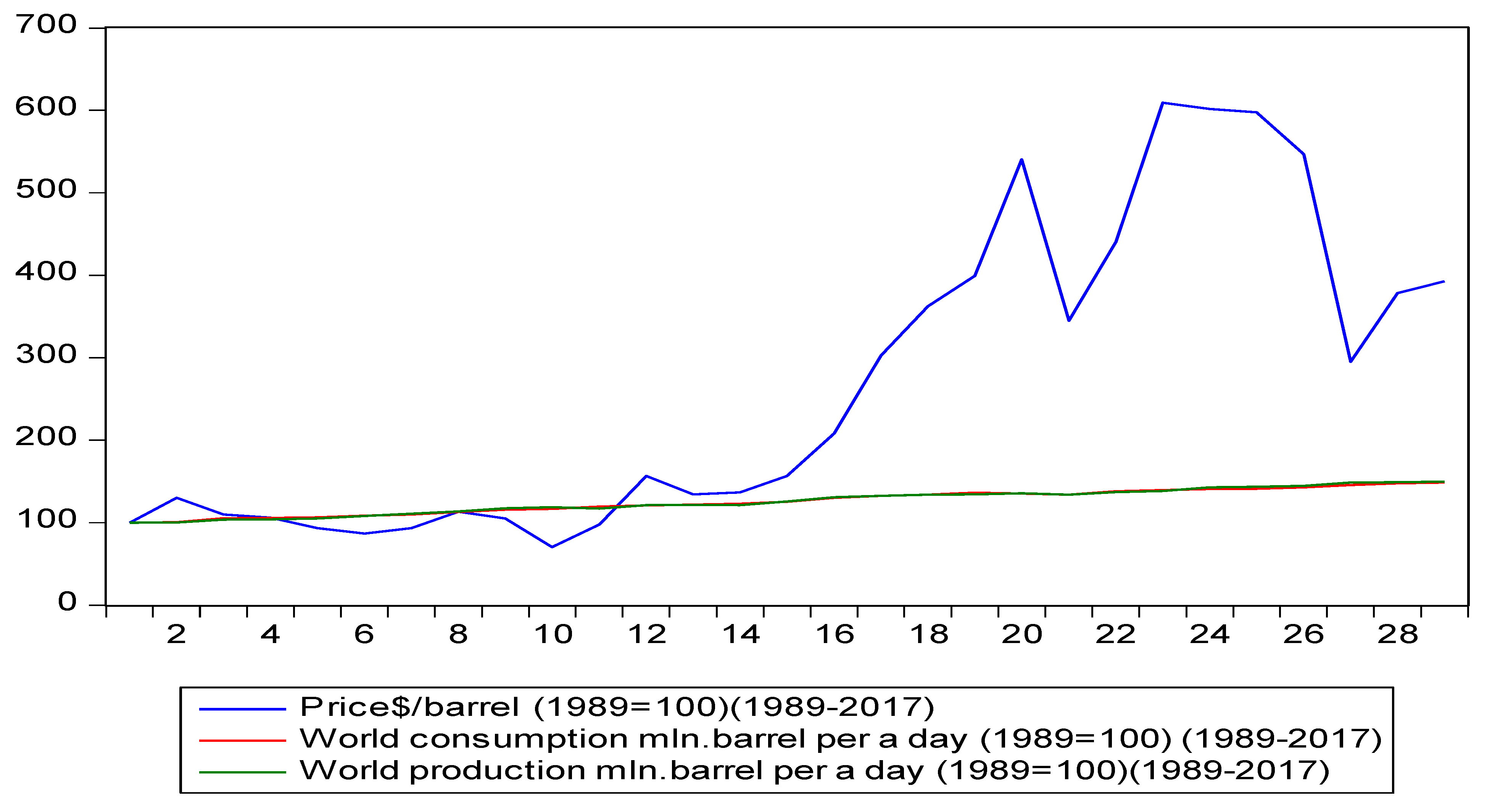
The necessity of scrutinizing the dependency of the production and consumption, literally supply and demand, in the world on the fluctuation of oil prices is waxing paramount because oil affects not only socio-economic processes but also political one. Thus, during 1989–2015 demand and supply in the world for oil constantly increased while we cannot say the same thing about oil prices. Therefore, recent changes in oil prices are divided into three phases and each of them are further divided into several stages. The first period encompasses 1989–1992, 1992–1996 and 1996–2000, the second period includes 2000–2003, 2003–2008 and 2008–2014 and the third period comprises the years 2014–2016. The changes in the price are closely related to the Gulf War in 1989–1992, while the reduction in oil prices in 1992–1996 was caused by political turmoil and the political realignment of the world. The plunge in oil prices was closely tied with economic crises in Russia and East Asian countries in 1996–2000 (Barings, England Bank, was symbolically sold for 1$ and the rouble came down twice in Russia and stock market was paralysed). Although a revival in the world market in 2000 caused the growth of oil prices, the following years resulted in a decline. However, the main reason of the fluctuation in oil prices—hitting the peak in 2008 and then plummeting afterwards—has been the recession in the mortgage and stock market as a driving factor of the economic crisis which commenced in 2008 but slackened relatively in 2011–2014. Furthermore, paramount events in the world politics have occurred recent years: crises in Ukraine and Syria.
Later it fluctuated around 60–65 $/barrel in 2016–2017. Analysing the first quarter of the oil price fluctuations we reveal that economic development is a motive for fluctuations besides political ones—the formation of oil demand in a real sector—and might cause a constant increase of GDP during this period. However, financial market indicators of GDP have to be considered, so modifications in the oil market, especially oil prices, reveal that it has already become one of the financial portfolios rather than a real commodity. This can be related with the expansion of futures operations in the oil market since 2000.
It is crystally clear that there are no any logical and economic relations between oil prices though we observe a dynamic compatibility in world GDP, industrial production, demand and supply of oil. We can come to a conclusion based on mathematical and economical models that reflect reciprocal relations among world GDP, demand and supply of oil and oil prices.
Research shows that although the oil production and consumption soared by 19–20% in 1989 compared to 2000, the oil price rocketed by 57%. These indicators were 37–38% and 610%, respectively. There is no need to comment on this. The main reason why we focus on 2011 is because of the highest oil prices and crisis in the Near East and the probability of the reduction of oil prices in the future that happened three years later.
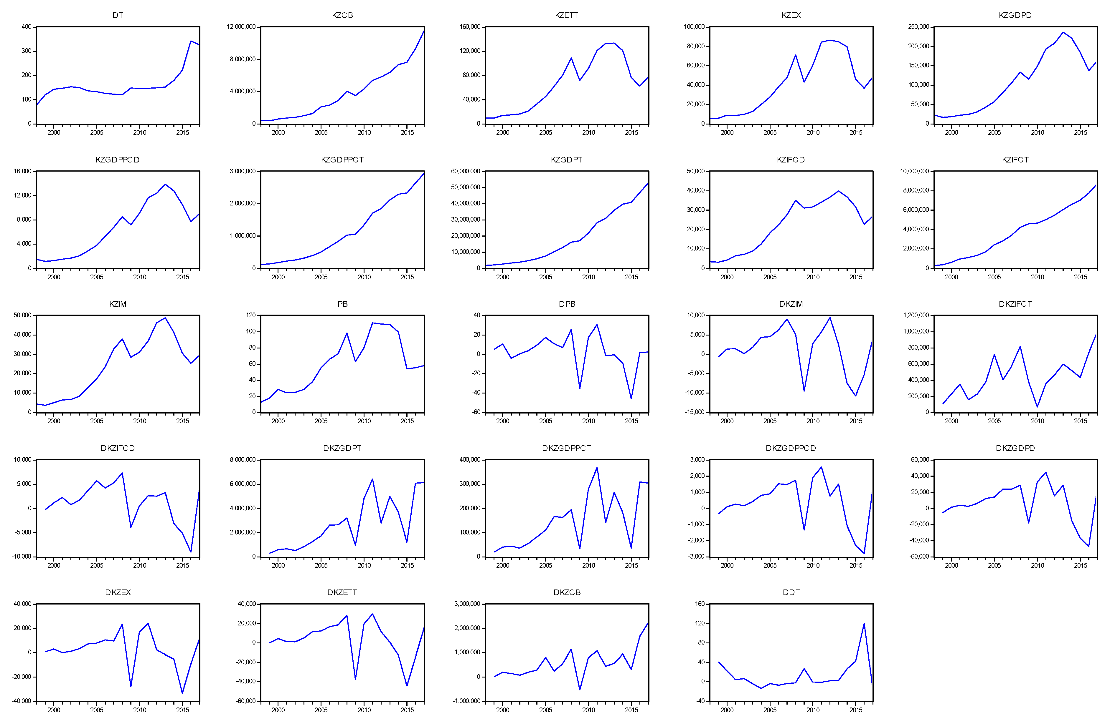
In general, models that illustrate the dependency among world GDP, world industry production, world oil consumption and production between 1989–2015 are evidence of what had been mentioned above.
3.2. Economic Development of Azerbaijan and Analysis of Oil Price (Factor)
Azerbaijan has maintained sustainable economic development and macroeconomic stability thanks to its socio-economic development strategy. As a result of the implementation of this strategy the diversification in the economy and the development of the non-oil sector as well as regions have been accelerated, the effective usage of strategical securities has been sustained and this has paved the way for a strong sustainable development foundation and the integration of the Azerbaijani economy into the world economic system and the well-being of its population.
Taking the case of 2000–2017, we can estimate a long-term increase in 2000–2008, a short-term decrease in 2008–2009 and an increase in 2009–2012 again. Afterwards, we can observe a slight decrease between 2012 and the first half of 2014 and a sharp decrease in 2014–2015. After the second half of 2014, the best period of oil prices has stopped. Oil prices have decreased approximately two-fold and led to the profitability of large-scale investment projects. In turn, it has made oil and gas companies who were in need of floating financial resources sell their assets (example, loan issuing by SOCAR, Azerbaijan).
If we design a graphic that illustrates the dynamics of oil on a yearly basis, it will be a polynomial linear graphic which paves the way for us to show realities. We can surmise that oil prices will fluctuate in a given time on a positive trend within the context of the sinusoid. It might be forecast that it would be relatively less reduction in 2015–2017 compared to 2013–2014. Afterwards, it will follow an increase in 2018–2021. However, this trend is useless in a real situation in order to forecast. Thus, oil prices exceeded the extreme point in 2013 and 2014 and since then, started going down. According to this, oil prices should have reduced up to 55.5 dollars at the beginning of 2016, but this situation wouldn’t be real.
The simpler economic interpretation embraces linear and exponential trends. The quality of this model is quite high and the determination coefficient is R2 > 0.87. It shows that researched oil prices depend on time. In the last 15 years oil prices have increased 6.78% on average, equivalent to 10.56 dollars.
The analysis of dynamics of oil prices reveals that oil prices declined drastically in economic crises periods (2008–2009 and 2014–2015). Thus, they decreased from 142 dollars in July to 42.8 dollars in December in 2008 (a nominal price decrease of 70%) while in 2014 they went down sharply from 110 dollars to 51 dollars in June and December, respectively (a decreased by 54%).
Price fluctuations for energy directly affect economic growth. This is confirmed by the dynamics of oil prices. Oil price hesitations influence the dynamics of macroeconomic indicators. Fluctuations of oil prices affect the revenue generated from crude oil exports and cause a large amount of investment (in the case prices soar upwards) or disappearing investment (in case prices plummet) and as a result, oil prices and indices for investment on fixed assets reflect its true value.
It is necessary to mention that the volume of the exports generated mainly from energy resources depends significantly on oil prices. Drops in oil price reduce the volume of the exports. For instance, as a result of the drop in oil prices by 55.4% in the 2008–2009 economic crises (from 139 to 62 dollars), exports greatly decreased. The consumer price index (CPI) increased up to 20.8% in 2008 and 10.1% in 2014. Thus, while oil price was decreasing in the market, the manat to dollar exchange rate was devaluated twice in 2014. However, since the Central Bank did not have policy and subjective factors in 2008–2009, the exchange rate of manat remained stable. As a result, 15 billion dollars was lost because of illegal operations by the International Bank in 2014–2015.
Thus, statistical analysis shows that key macroeconomic indicators depend on exporting energy resources. It features raw material resources of Azerbaijan economy. Unlike Azerbaijan, in Russia not only a drop in oil prices but also the complex geopolitical situation, sanctions by Western countries and the response by Russia exacerbated macroeconomic indicators: limited penetration into the financial markets of Western countries, prohibition to export some state-of-the-art technologies to Russia, reduction in foreign investment and uncertainty in business environment.
Recently, the Azerbaijani economy and some of its macroeconomic indicators have been affected by unstable situations happening in the world economy. Investment, oil production and oil price indicators are worthwhile when we analyze economic development in terms of sources in the Republic. Thus, we can witness that those indicators emerge as macroeconomic indicators and main economic factors in the analysis of international finance organization. That is why we have taken these factors into consideration.
4. Methodology and Econometric Models
Model Specification
Initially, we have checked the stationarity of time series and have converted them from non-stationary into stationary. We have conducted a single root test. Having used macroeconomic indicators, we have established separate and combined models that indicate the dependency of world oil prices on the world GDP, world industry production, daily oil production and consumption (demand). Furthermore, we have established models that reflect the dependency of world oil price and oil production volume based on the macroeconomic indicators of Azerbaijan and Kazakhstan.
There is a regression equation for variables which are originally stationary in the first phase and simultaneously are differentiated stationary. We have to note that there is a calculation for stationary checking (single root tests) below:
In this equation, and represent regression coefficients, and —independent and dependent values, —white noise error, and represents time. Having completed the regression equation, the next step is checking the action of white noise error. If εt is stationary, it means variables possess co-integration links and they are not spurious. That is why Equation (1) is considered a long-term equation. The last step is to evaulate ECM by using white noise error () and stationary variables for checking the dependency and direction of cause and effect relations:
We will use error correction model (ECM). The formula is as follows:
This is the ECM structure with two variables (one dependent and the other one independent variable) in the equation. Here, is the dependent variable, is the independent and explanatory variable. shows the constant term of the model and means the white noise error. indicates long-term and and short-term period coefficients. If coefficient is θ statistically significance and negative, then we can consider the co-integration relation as constant. It means that digressions for a long-term or balance in a short-term are temporary and will be corrected in the long-term. It must be noted that is expected to be −1 and 0.
Having proven the co-integration relationship among variables, long-term coefficients will be assessed in the next phase. We can calculate it in terms of y when the coefficients in the long-term in equation are zero ( = 0):
Later, we can check the stability of co-integration relation by reassessing it instead of long-term coefficient part () in Equation (1) by calculating the long-term white noise error (ECTT). In other words, the formula of the model will be as follows:
If n−1 = p and m−1 = q:
Let’s accept p = 0; q = 0 and set up simple linear correction model and analyze it:
While analyzing the work of Engle and Granger, the main problem that we encounter is the assessment of the co-integration equation (see Equation (1)) in a short and long term and finding alternative methods.
While developing the test, Granger and Engle [80] considered that assessment results obtained through the OSL method are consistent and efficient. However, the explanation of coefficients obtained through OSL is not right based on traditional t-statistics, because, dynamic forms in the static equation and standard errors are not included and inclined. Especially, this inclination is high in small-sized samples [81]. In order to solve the problem, there have been different approaches and assessment methods [82,83,84]. We do not provided detailed information here because this has been elabored by Utkulu [85]. Inder [86] mentioned that we had better use dynamic models rather than correction of long-term coefficients. Moreover, Stock and Vatson [87] indicated that DOLS (based on Monte Carlo simulations) performed better than other alternative methods for small-sized groups. For getting precise results, the Engle-Graner cointegration equation has been assessed using FMOLS and DOSL as well as CCR methods in this article.
There is a lot of information about the stationary and significance of variables in time series analysis in modern econometric books [88,89,90]. First of all, the stationarity of time series has been checked and tested though three commonly‒accepted tests (Augmented Dickey-Fuller—ADF; Phillips-Perron—PP and Kwiatkowski-Phillips-Schmidt-Shin—KPSS). Tests have been done through the EVIEWS 9 software. Fully Modified Ordinary Least Squares (FMOLS) is one of the alternative co-integration methods proposed by Phillips and Hansen [82] FMOLS realizes an auto-correction of the problems created from endogenic and consecutive correlations which are supposed to be considered in econometric assessments. Dynamic Ordinary Least Squares method (DOLS) has been proposed by Stock and Watson as an asymptotic efficient assessment tool [87]. This method offers an assessment methodology for eliminating endogenic problems or mutual impact in co-integration systems. Canonic co-integration regression (CCR) has been developed by Park [91] and is very close to FMOLS. It enables us to obtain asymptotic efficient results while assessing through OLS.
It must be considered that there is a complex assessment rule of this co-integrated method and the mathematical calculation of Phillips and Hansen [83], Stock and Watson (DOSL) [87] Philips-Ouliaris [92] that will not be covered in details here. There is a regression equation for variables which are originally stationary in the first phase and simultaneously are differentiated stationarily. We have to note that there is a calculation for stationarity checking (single root tests) below: in terms of checking the reliability of results, Musayev and Aliyev have assessed variables through FMOLS, DOLS and CCR co-integration methods [93,94].
5. Empirical Results and Discussion
5.1. Results Unit Root Test
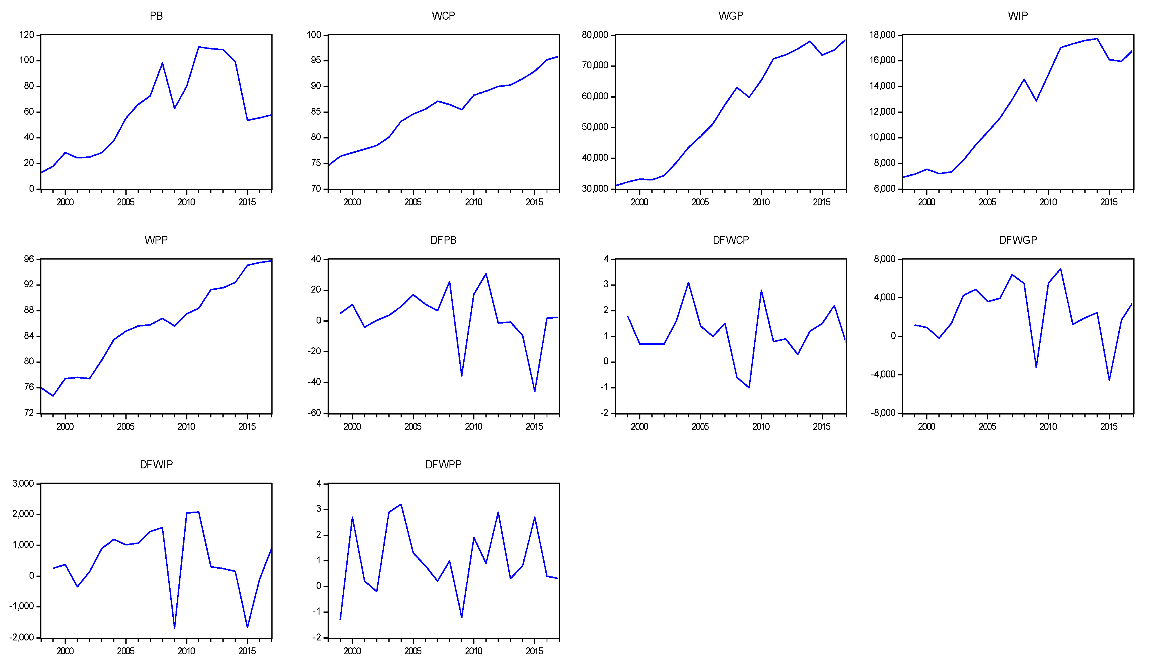
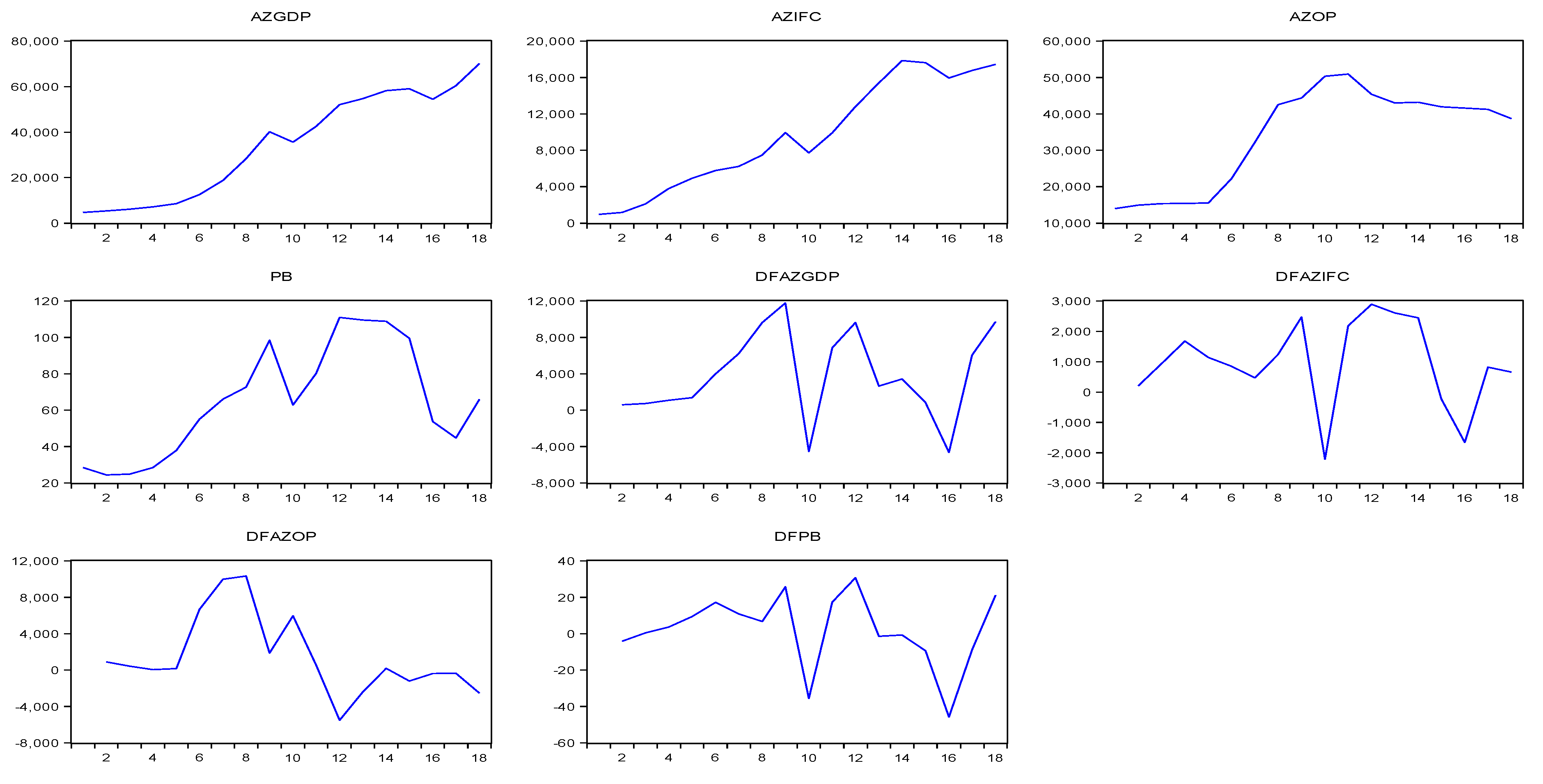
ADF reveals that world GDP, world industry production, oil prices, world oil production (supply) and world oil consumption (demand) are in the 1st difference and stationary in three cases (constant; constant and linear trend; none). Only world GDP in the 1st difference is not stationary in one case (none). This result is suitable for the method. The PP result is similar to the ADF test, but it is a bit unclear (Table A8.W, Table A9.W, Table A10.W and Table A11.W.) Thus, world GDP and oil process are stationary (none) both in 1st difference and in simple case. KPSS test is also unclear. The abovementioned facts might be referred to time series tests of the Azerbaijan and Kazakhstan macroeconomic indicators. However, three time series (azpcim, azpcipcm, dm) are stationary in the 2nd difference of ADF and PP significance test (Table A12.AZ, Table A13.AZ, Table A14.AZ, Table A15.AZ and Table A16.AZ; Table A23.KZ, Table A24.KZ and Table A25.KZ).
5.2. Empirical Results
The coefficients of only two of the models (models 1 and 2) that reflect the impact of World GDP, world industry production, daily oil production (supply) and oil consumption (demand) on oil price are statistically significant. In other words, world GDP and world industry production influence on world oil prices (Table 1). It can be inferred that model 3 and 4 has no any impact of world daily oil production (supply) and oil consumption (demand) on world oil prices, so we can infer that although world industry production plays a certain role in world oil price fluctuation and world GDP, daily oil production (supply) and oil consumption (demand) don’t impact the world oil price. As mentioned at the beginning of the study, non-economic factors play a role in oil price fluctuations (up and down).
The models (model 5–8) reflecting the dependency of investment on fixed assets on oil price and oil production in Azerbaijan show the adverse process (Table 2). Thus, models 5 and 7 are either constant or the oil price coefficient is statically significant. Generally, the model is significant and adequate. However, models 6 and 8 (models that reflect the dependency of oil price on Azerbaijan GDP and investment in fixed capital) are not statistically significant (reflecting the oil production coefficient in Azerbaijan) and generally, the models are not adequate. This gives an evidence once more that Azerbaijan’s GDP and investment in fixed capital depends entirely on the oil price and does not depend on the volume of oil production in Azerbaijan (mainly in the short-term).
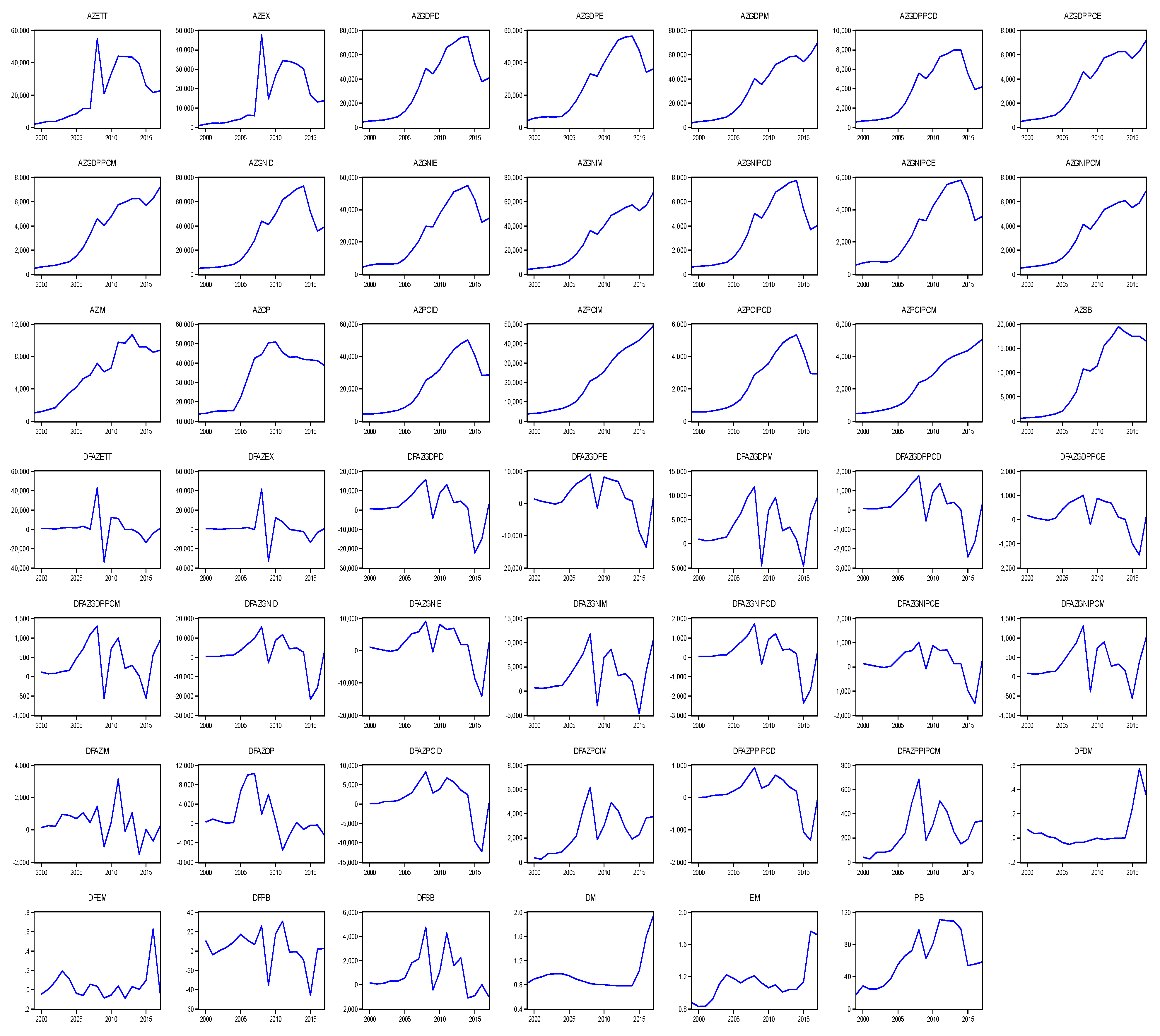
The macroeconomic indicators of the Azerbaijani manat and the models (models 11, 14, 17, 18 and 21) expressed in figures from the models reflecting the influence of oil prices on macroeconomic indicators in Azerbaijan (model 9–31) are statistically significant and the models are adequate (Table 3, Table 4 and Table 5). However, these indicators are expressed in models that are dependent on oil prices (models 9,10,12,13,15,16,19,20,22–25,30), either in euros or in dollars, but the macroeconomic indicators are statistically significant, and the constants are negligible. These models are adequate. In these models, the weakness of the contacts can be attributed to the relative stability of the foreign currencies (euro and dollar) against the Azerbaijani manat in a long term by 2015. But the latter is a completely different case and reflects oil and gas prices in Azerbaijan that show the dependence of the Azerbaijani manat on the euro and the dollar (models 27–29). Here, both the oil prices and the coefficients of the models are not statistically significant, and the models are inadequate. The reason might be the weakness of the relation between oil production and oil prices in Azerbaijan. The inadequacy of model 28 and model 29 encompasses the relationship between exchange rates and oil prices, can be related with the permanent depreciation of the Azerbaijani manat against foreign currencies, mainly against the euro and the dollar, by 2015. Thus, the results of these models (models 1–31) once again prove that the relationship between oil prices and many macroeconomic indicators is different in oil exporting and oil importing countries.
The following models (model 32–42) show the abovementioned results regarding the dependency of macroeconomic indicators on oil factor of the Republic of Kazakhstan (Table 6 and Table 7). The dependency of foreign trade turnover of Kazakhstan on the import and export oil price (model 33,34,39) is very important. Thus, the main export product of the Republic is oil and oil products and they are traded in dollars. However, the coefficient of the model (model 32) which features the dependency of the ratio of national currency “tenge” to the dollar on oil prices is not statistically significant. The reason for this is the regulation of dollar/tenge exchange rate by the state, so the influence of oil on macroeconomic indicators is similar to the impact of oil price on Azerbaijani macroeconomic indicators.
It is essential to evaluate the results with FMOLS, DOLS and CCR co-integration in term of double checking the reliability of obtained corollaries (Table 8, Table 9, Table 10, Table 11, Table 12, Table 13, Table 14, Table 15, Table 16, Table 17 and Table 18).
In addition, we carried out post-diagnostic tests such as serial correlation and heteroskedasticity by conducting Breusch-Godfrey LM and Breusch-Pagan-Godfrey tests, respectively. We further check for the specification error and the distribution of the error term by conducting Ramsey RESET and Jarque-Bera tests, respectively. Thus, the results for the tests are presented in Table A28 (diagnostic test results). The post-diagnostic test results revealed that, the null hypotheses of no serial correlation, no misspecification error, no heteroscedasticity and normally distributed error term cannot be rejected. Thus, almost all models are viable and robust in satisfying the assumption of the classical linear regression model. The robustness tests of the almost all models revealed that the Breusch-Godfrey serial correlation LM test, heteroscedasticity test, Ramsey RESET specification test and Jarque-Bera normality test had correct functional form and the model’s residuals were serially unrelated, normally distributed and homoscedastic.
6. Conclusions
The main idea that we put forward is to reveal the potential capacity if Azerbaijan embarks on exploiting new and high-yielding deposits. As a result of this exploitation, the production will affect economic growth in a short, medium and long term. Meanwhile, it has better researched a number of macroeconomic indicators in 2008 and 2014, respectively, in Azerbaijan in terms of getting more information about the effects of the oil boom on economic development not only in a short term but also in a medium and long term. Those steps pave the way for understanding the general dynamics of economic development either in terms of its structure or quality.
Our study examined the impact of oil resources both in quantity and in price on the world’s and Azerbaijan’s economic growth. Ostensibly, the impact of oil price on oil-importing countries is indirect but direct on oil-exporting countries.
In our research, we witnessed the fluctuation of world GDP, world industry production, world oil production (daily) and world oil consumption (daily) according to the oil price in the world oil market in 2008–2009. Furthermore, the abovementioned macroeconomic indicators are closely linked with the fall of oil prices in 2014–2015. These processes continued in 2017–2018, respectively.
We notice the same situation but more effectively in the case of Azerbaijan. The main reason for this is that Azerbaijan depends heavily on oil and oil products in its exports (80–90%). Because GDP (in money) increased constantly during the research period, this growth had been high in 2008 but reduced in 2009. The oil price decreased twice during this period (2008–2009). Meanwhile, a series of global political events in 2014 caused a decrease in Azerbaijan’s GDP, GNI, investment in fixed assets, including GDP per capita, GNI in euros and dollars and people’s income in dollars. Thus, the value of the Azerbaijani manat was devaluated twice when oil price fell twice and its value changed from 0.78 USD to 1.65 USD. It proves that Azerbaijan economy depends on oil factors.
All the abovementioned factors were proved by the results of econometric models. These have been comprehensively illustrated in simple models that reflect the dependency of Azerbaijan’s currency in euros and dollars on the oil price.
Obviously, economic growth in the post‒peak period of the production occurs under the influence of GDP and oil income policy. This aspect must be considered as an assessment of certain indicators of economic growth in Azerbaijan, as well as setting economic policy measures in the post-peak production period and in the discussions of the low growth rate of the oil economy.
It must be noted that not only political issues but also economic growth stand on the root of the fluctuations that directly affect the first period of oil price changes. Thus, demand for oil is being formed in a real sector. However, world GDP has increased steadily. It can’t be forgetten that financial market indicators are reflected in GDP. Hence, fluctuations in oil markets, in other words oil price changes, mean that oil has already changed from a real commodity into a financial portfolio. The reasoning of models from either an economic or mathematical point of view can closely be related to the relative proximity of the economic growth rate with oil production and price rate. Unlike the world economic situation, as noted above, there is no absolute dependency between world oil production and consumption as well as the relative dependency among world oil production, consumption and world GDP and in general, the dependency between oil price and these factors (world oil production, consumption and world GDP), especially in the last decade. That’s why our republic also witnessed the reverse processes. Although economic growth and demand act as an important factor in the world oil price, it can be inferred that the economic growth observed in Azerbaijan, one of the smallest exporters of oil production in the world, is largely dependent on oil production and oil prices.
We can mention the same results about Khazakstan. Thus, the dependency of macroeconomic indicators on oil price of the Republic of Kazakhstan can be easily seen in foreign trade turnover and import and export. As occurs in Azerbaijan, although the dependency of national currency (dollar/tenge) on oil price is too strong, the essence of the regulation of dollar/tenge exchange rate is a bit hidden. However, if the Central Bank hadn’t conducted currency interventions, the exchange rate might have been real either in Azerbaijan or in Khazakhstan, so the influence of oil on the macroeconomic indicators of Azerbaijan is similar to the impact of oil price on macroeconomic indicators. The dollar/manat and tenge/manat exchange has been stable for 10 years due to the intervention in the market in Azerbaijan and Khazakhstan). This has caused some distortions in macroeconomic indicators. We can also witness it in GDP and GNP in dollars and manat for the last 3 years. Our conclusion supports that market intervention must be weak. Moreover, we think that the main indicators of the economic situation must be foreign trade turnover since both Azerbaijan and Khazakhstan are oil-exporting countries.
Author Contributions
Conceptualization, N.Q.-O.H. and S.İ.H.; Formal analysis, N.Q.-O.H. and S.İ.H.; Methodology, N.Q.-O.H. and S.İ.H.; Supervision, N.Q.-O.H. and S.İ.H.; Validation, N.Q.-O.H. and S.İ.H.; Writing—original draft, N.Q.-O.H. and S.İ.H.; Writing—review & editing, N.Q.-O.H. and S.İ.H.
Funding
This research received no external funding.
Conflicts of Interest
The author declares no conflict of interest.
Appendix A

Table A1.
Abbreviations and internet resources.
| wgdp | World Gross Domestic Product, dollar | mln. dollar | www.ycharts.com |
| wip | Industrial Production, dollar | mln. dollar | www.ycharts.com |
| wpp | World Production, barrel per a day | mln. barrel | www.ycharts.com |
| wcp | World Consumption, barrel per a day | mln. barrel | www.ycharts.com |
| pb | Oil Prices | $/Barrel | www.ycharts.com |
| azgdp | Azerbaijan Gross Domestic Product, manat | mln. manat | www.stat.gov.az |
| azifc | Azerbaijan Investment On Fixed Capital, manat | mln. manat | www.stat.gov.az |
| azop | Azerbaijan Oil Production, ton | mln. ton | www.stat.gov.az |
| azgdpm | Azerbaijan Gross Domestic Product, manat | mln. manat | www.stat.gov.az |
| azgdpd | Azerbaijan Gross Domestic Product, dollar | mln. dollar | www.stat.gov.az |
| azgdpe | Azerbaijan Gross Domestic Product, euro | mln. euro | www.stat.gov.az |
| azgdppcm | Azerbaijan Gross Domestic Product - Per Capita, manat | manat | www.stat.gov.az |
| azgdppcd | Azerbaijan Gross Domestic Product - Per Capita, dollar | dollar | www.stat.gov.az |
| azgdppce | Azerbaijan Gross Domestic Product - Per Capita, euro | euro | www.stat.gov.az |
| dm | 1$ = manat | www.stat.gov.az | |
| em | 1€ = manat | www.stat.gov.az | |
| azgnim | Azerbaijan Gross National Income, manat | mln. manat | www.stat.gov.az |
| azgnid | Azerbaijan Gross National Income, dollar | mln. dollar | www.stat.gov.az |
| azgnie | Azerbaijan Gross National Income, euro | mln. euro | www.stat.gov.az |
| azgnipcm | Azerbaijan Gross National Income, Per Capita, manat | manat | www.stat.gov.az |
| azgnipcd | Azerbaijan Gross National Income, Per Capita, dollar | dollar | www.stat.gov.az |
| azgnipce | Azerbaijan Gross National Income, Per Capita, euro | euro | www.stat.gov.az |
| azpcim | Azerbaijan Per Capita Income, manat | mln. manat | www.stat.gov.az |
| azpcid | Azerbaijan Per Capita Income, dollar | mln. dollar | www.stat.gov.az |
| azpcipcm | Azerbaijan Per Capita Income, Per Capita, manat | manat | www.stat.gov.az |
| azpcipcd | Azerbaijan Per Capita Income, Per Capita, dollar | dollar | www.stat.gov.az |
| azcb | Azerbaijan state budget, manat | mln. manat | www.stat.gov.az |
| azett | Azerbaijan External A Trade Turnover, dollar | mln. dollar | www.stat.gov.az |
| azim | Azerbaijan, Import, dollar | mln. dollar | www.stat.gov.az |
| azex | Azerbaijan, Export, dollar | mln. dollar | www.stat.gov.az |
| kzdt | 1$ = tenge | www.stat.gov.kz | |
| kzett | Kazakhstan External A Trade Turnover, dollar | mln. dollar | www.stat.gov.kz |
| kzex | Kazakhstan Export, dollar | mln. dollar | www.stat.gov.kz |
| kzgdpd | Kazakhstan Gross Domestic Product, dollar | mln. dollar | www.stat.gov.kz |
| kzgdpt | Kazakhstan Gross Domestic Product, tenge | mln.tenge | www.stat.gov.kz |
| kzgdppcd | Kazakhstan Gross Domestic Product - Per Capita dollar | mln. dollar | www.stat.gov.kz |
| kzgdppct | Kazakhstan Gross Domestic Product - Per Capita tenge | mln.tenge | www.stat.gov.kz |
| kzim | Kazakhstan Import, dollar | mln. dollar | www.stat.gov.kz |
| kzifcd | Kazakhstan Investment On Fixed Capital, dollar | mln. dollar | www.stat.gov.kz |
| kzifct | Kazakhstan Investment On Fixed Capital, tenge | mln.tenge | www.stat.gov.kz |
| kzcb | Kazakhstan state budget | mln.tenge | www.stat.gov.kz |
Table A2.
W. Descriptive statistics.
| PB | WCP | WGP | WIP | WPP | |
|---|---|---|---|---|---|
| Mean | 60.29000 | 85.51500 | 55870.85 | 12492.33 | 85.65500 |
| Median | 56.70000 | 86.05000 | 58661.50 | 12935.50 | 85.70000 |
| Maximum | 110.9000 | 95.90000 | 78855.00 | 17737.60 | 95.80000 |
| Minimum | 12.80000 | 74.60000 | 31123.00 | 6920.200 | 74.70000 |
| Std. Dev. | 32.55612 | 6.398542 | 17843.94 | 4123.350 | 6.737521 |
| Skewness | 0.216260 | −0.143336 | −0.139143 | −0.126362 | −0.081289 |
| Kurtosis | 1.799477 | 1.949325 | 1.442792 | 1.421026 | 1.876194 |
| Jarque‒Bera | 1.356940 | 0.988415 | 2.085282 | 2.130857 | 1.074477 |
| Probability | 0.507393 | 0.610054 | 0.352522 | 0.344580 | 0.584360 |
| Sum | 1205.800 | 1710.300 | 1117417. | 249846.6 | 1713.100 |
| Sum Sq. Dev. | 20138.12 | 777.8855 | 6.05E + 09 | 3.23E + 08 | 862.4895 |
| Observations | 20 | 20 | 20 | 20 | 20 |
Table A3.
AZ. Descriptive statistics.
| AZGDP | AZOP | AZIFC | PB | |
|---|---|---|---|---|
| Mean | 34364.88 | 34041.50 | 9657.839 | 65.13889 |
| Median | 37869.35 | 41396.50 | 8815.300 | 64.35000 |
| Maximum | 70135.10 | 50900.00 | 17850.80 | 110.9000 |
| Minimum | 4718.100 | 14017.00 | 967.8000 | 24.40000 |
| Std. Dev. | 23076.50 | 13644.19 | 6044.385 | 30.57966 |
| Skewness | −0.051100 | −0.497386 | 0.063590 | 0.180543 |
| Kurtosis | 1.457302 | 1.588056 | 1.574118 | 1.730362 |
| Jarque‒Bera | 1.792771 | 2.237368 | 1.536985 | 1.306773 |
| Probability | 0.408042 | 0.326709 | 0.463712 | 0.520281 |
| Sum | 618567.9 | 612747.0 | 173841.1 | 1172.500 |
| Sum Sq. Dev. | 9.05E+09 | 3.16E + 09 | 6.21E + 08 | 15896.96 |
| Observations | 18 | 18 | 18 | 18 |
Table A4.
AZ. Descriptive statistics.
| AZETT | AZEX | AZGDPD | AZGDPE | AZGDPM | AZGDPPCD | AZGDPPCE | AZGDPPCM | |
|---|---|---|---|---|---|---|---|---|
| Mean | 21404.16 | 15489.87 | 35143.77 | 27619.00 | 32754.89 | 3874.879 | 3589.532 | 3589.532 |
| Median | 20824.50 | 13118.40 | 37862.80 | 31738.90 | 35601.50 | 3928.600 | 4033.200 | 4033.200 |
| Maximum | 54926.00 | 47756.00 | 75234.70 | 56581.10 | 70135.10 | 7990.800 | 7205.000 | 7205.000 |
| Minimum | 1965.100 | 929.7000 | 4583.700 | 4299.200 | 3775.100 | 582.9000 | 480.1000 | 480.1000 |
| Std. Dev. | 17122.27 | 14441.52 | 25719.56 | 19243.98 | 23498.71 | 2744.927 | 2444.384 | 2444.384 |
| Skewness | 0.493867 | 0.748419 | 0.170239 | 0.142051 | 0.039976 | 0.152959 | −0.051644 | −0.051644 |
| Kurtosis | 1.880120 | 2.300460 | 1.601742 | 1.535312 | 1.426008 | 1.575645 | 1.370876 | 1.370876 |
| Jarque‒Bera | 1.765219 | 2.161152 | 1.639581 | 1.762270 | 1.966376 | 1.680212 | 2.109564 | 2.109564 |
| Probability | 0.413702 | 0.339400 | 0.440524 | 0.414312 | 0.374116 | 0.431665 | 0.348268 | 0.348268 |
| Sum | 406679.0 | 294307.5 | 667731.6 | 524761.0 | 622343.0 | 73622.70 | 68201.10 | 68201.10 |
| Sum Sq. Dev. | 5.28E + 09 | 3.75E + 09 | 1.19E + 10 | 6.67E + 09 | 9.94E + 09 | 1.36E + 08 | 1.08E + 08 | 1.08E + 08 |
| Observations | 19 | 19 | 19 | 19 | 19 | 19 | 19 | 19 |
Table A5.
AZ. Descriptive statistics.
| AZGNID | AZGNIE | AZGNIM | AZGNIPCD | AZGNIPCE | AZGNIPCM | AZIM | AZOP | |
|---|---|---|---|---|---|---|---|---|
| Mean | 32977.46 | 25961.72 | 30784.81 | 3633.311 | 2859.437 | 3370.984 | 5914.316 | 32970.63 |
| Median | 35587.40 | 29396.00 | 32973.50 | 3692.500 | 3330.100 | 3735.400 | 6123.100 | 41223.00 |
| Maximum | 73078.00 | 54959.20 | 67439.50 | 7761.700 | 5837.300 | 6928.100 | 10712.50 | 50900.00 |
| Minimum | 4770.500 | 4474.400 | 3929.000 | 606.7000 | 569.1000 | 499.7000 | 1035.900 | 13695.00 |
| Std. Dev. | 24451.35 | 18365.40 | 22450.31 | 2603.014 | 1931.598 | 2330.771 | 3290.659 | 14057.38 |
| Skewness | 0.229488 | 0.206398 | 0.103460 | 0.212549 | 0.188575 | 0.015960 | −0.175844 | −0.366667 |
| Kurtosis | 1.638196 | 1.556892 | 1.439041 | 1.610780 | 1.556055 | 1.376323 | 1.627825 | 1.432792 |
| Jarque-Bera | 1.634927 | 1.783595 | 1.962867 | 1.670924 | 1.763216 | 2.087899 | 1.588517 | 2.370187 |
| Probability | 0.441550 | 0.409918 | 0.374774 | 0.433674 | 0.414116 | 0.352061 | 0.451916 | 0.305718 |
| Sum | 626571.7 | 493272.6 | 584911.3 | 69032.90 | 54329.30 | 64048.70 | 112372.0 | 626442.0 |
| Sum Sq. Dev. | 1.08E + 10 | 6.07E + 09 | 9.07E + 09 | 1.22E + 08 | 67159252 | 97784883 | 1.95E + 08 | 3.56E + 09 |
| Observations | 19 | 19 | 19 | 19 | 19 | 19 | 19 | 19 |
Table A6.
AZ. Descriptive statistics.
| AZPCID | AZPCIM | AZPCIPCD | AZPCIPCM | AZSB | PB | EM | DM | |
|---|---|---|---|---|---|---|---|---|
| Mean | 22753.22 | 21567.54 | 2505.347 | 2359.195 | 9080.063 | 62.78947 | 1.130816 | 0.969505 |
| Median | 25237.80 | 20735.40 | 2894.700 | 2378.300 | 10325.90 | 57.90000 | 1.111100 | 0.893400 |
| Maximum | 50321.50 | 49162.90 | 5344.700 | 5050.500 | 19496.30 | 110.9000 | 1.765900 | 1.942300 |
| Minimum | 4477.500 | 3687.700 | 568.7000 | 468.5000 | 559.5000 | 17.80000 | 0.829600 | 0.784400 |
| Std. Dev. | 16373.29 | 16019.94 | 1722.995 | 1644.748 | 7440.780 | 31.41489 | 0.246655 | 0.298254 |
| Skewness | 0.270434 | 0.323499 | 0.253323 | 0.235758 | 0.090082 | 0.205825 | 1.447596 | 2.418062 |
| Kurtosis | 1.631916 | 1.601747 | 1.619175 | 1.509350 | 1.313213 | 1.783266 | 4.858842 | 7.831108 |
| Jarque‒Bera | 1.713319 | 1.879193 | 1.712666 | 1.935123 | 2.278186 | 1.306169 | 9.371298 | 36.99276 |
| Probability | 0.424578 | 0.390785 | 0.424717 | 0.380009 | 0.320109 | 0.520438 | 0.009227 | 0.000000 |
| Sum | 432311.1 | 409783.3 | 47601.60 | 44824.70 | 172521.2 | 1193.000 | 21.48550 | 18.42060 |
| Sum Sq. Dev. | 4.83E + 09 | 4.62E + 09 | 53436840 | 48693500 | 9.97E + 08 | 17764.12 | 1.095092 | 1.601201 |
| Observations | 19 | 19 | 19 | 19 | 19 | 19 | 19 | 19 |
Table A7.
Models.
| Model 1 | |
| Model 2 | |
| Model 3 | |
| Model 4 | |
| Model 5 | |
| Model 6 | |
| Model 7 | |
| Model 8 | |
| Model 9 | |
| Model 10 | |
| Model 11 | |
| Model 12 | |
| Model 13 | |
| Model 14 | |
| Model 15 | |
| Model 16 | |
| Model 17 | |
| Model 18 | |
| Model 19 | |
| Model 20 | |
| Model 21 | |
| Model 22 | |
| Model 23 | |
| Model 24 | |
| Model 25 | |
| Model 26 | |
| Model 27 | |
| Model 28 | |
| Model 29 | |
| Model 30 | |
| Model 31 | |
| Model 32 | |
| Model 33 | |
| Model 34 | |
| Model 35 | |
| Model 36 | |
| Model 37 | |
| Model 38 | |
| Model 39 | |
| Model 40 | |
| Model 41 | |
| Model 42 |
Table A8.
W. The Unit Root test results.
| The ADF Test | ||||||||||||
|---|---|---|---|---|---|---|---|---|---|---|---|---|
| Level | 1st Difference | |||||||||||
| Constant | k | Constant, Linear Trend | k | None | k | Constant | k | Constant, Linear Trend | k | None | k | |
| pb | −1.696 | 0 | −1.169 | 0 | −0.263 | 0 | −4.101 *** | 0 | −4.333 ** | 0 | −4.163 *** | 0 |
| wgdp | −0.554 | 0 | −1.553 | 0 | 3.095 | 0 | −3.712 ** | 0 | −3.311 * | 1 | ‒0.759 | 2 |
| wip | −0.873 | 0 | −1.409 | 0 | 1.799 | 0 | −3.761 ** | 0 | −3.719 ** | 0 | −3.128 *** | 0 |
| wcp | −0.569 | 0 | −2.175 | 0 | 4.771 | 0 | −3.950 *** | 0 | −3.825 ** | 0 | −2.350 ** | 0 |
| wpp | −0.299 | 0 | −2.866 | 0 | 3.304 | 0 | −5.336 *** | 0 | −5.145 *** | 0 | −3.045 *** | 0 |
Note: ADF denotes the Augmented Dickey‒Fuller single root system respectively. The maximum lag order is 3. The optimum lag order is selected based on the Shwarz criterion automatically; ***, ** and * indicate rejection of the null hypotheses at the 1%, 5% and 10% significance levels, respectively. The critical values are taken from MacKinnon [95]. Assessment period: 1999–2017.
Table A9.
W. The Unit Root test results.
| The PP Test | ||||||||||||
|---|---|---|---|---|---|---|---|---|---|---|---|---|
| Level | 1st Difference | |||||||||||
| Constant | k | Constant, Linear Trend | k | None | k | Constant | k | Constant, Linear Trend | k | None | k | |
| pb | −1.701 | 1 | −1.168 | 0 | −0.265 | 1 | −4.101 *** | 1 | −4.503 ** | 3 | −4.163 *** | 1 |
| wgdp | −0.552 | 3 | −1.553 | 0 | 3.095 *** | 0 | −3.676 ** | 5 | −3.593 * | 6 | −2.423 ** | 2 |
| wip | −0.869 | 2 | −1.409 | 0 | 1.647 * | 1 | −3.738 ** | 3 | −3.679 * | 3 | −3.125 *** | 1 |
| wcp | −0.551 | 3 | −2.292 | 1 | 5.450 | 3 | −4.000 *** | 3 | −3.838 ** | 3 | −2.305 ** | 1 |
| wpp | −0.135 | 3 | −2.866 | 0 | 4.412 | 3 | −5.589 ** | 3 | −5.409 *** | 3 | −3.048 *** | 1 |
Note: PP Phillips-Perron is single root system. The optimum lag order in PP test is selected based on the Newey-West criterion automatically; ***, ** and * indicate rejection of the null hypotheses at the 1%, 5% and 10% significance levels, respectively. The critical values are taken from MacKinnon [95]. Assessment period: 1999–2017.
Table A10.
W. The Unit Root test results.
| The KPSS Test | ||||||||
|---|---|---|---|---|---|---|---|---|
| Level | 1st Difference | |||||||
| Constant | k | Constant, Linear Trend | k | Constant | k | Constant, Linear Trend | k | |
| pb | 0.417 * | 3 | 0.145 * | 2 | 0.233 | 2 | 0.162 ** | 5 |
| wgdp | 0.585 ** | 3 | 0.116 | 2 | 0.134 | 3 | 0.127 * | 3 |
| wip | 0.563 ** | 3 | 0.116 | 2 | 0.145 | 2 | 0.120 * | 3 |
| wcp | 0.611 ** | 3 | 0.101 | 2 | 0.119 | 3 | 0.109 | 3 |
| wpp | 0.601 ** | 3 | 0.075 | 1 | 0.090 | 3 | 0.089 | 3 |
Note: KPSS denotes Kwiatkowski-Phillips-Schmidt-Shin single root system. The optimum lag order in KPSS test is selected based on the Newey-West criterion automatically; ***, ** and * indicate rejection of the null hypotheses at the 1%, 5% and 10% significance levels, respectively. The critical values are taken from Kwiatkowski-Phillips-Schmidt-Shin [96]. Assessment period: 1999–2017.
Table A11.
AZ. The Unit Root test results.
| The ADF Test | ||||||||||||
|---|---|---|---|---|---|---|---|---|---|---|---|---|
| Level | 1st Difference | |||||||||||
| Constant | k | Constant, Linear Trend | k | None | k | Constant | k | Constant, Linear Trend | k | None | k | |
| pb | −1.627 | 0 | −1.378 | 0 | −0.259 | 0 | −3.523 ** | 0 | −3.640 * | 1 | −3.597 *** | 0 |
| azgdp | 0.062 | 0 | −2.223 | 0 | 2.552 | 0 | −3.332 ** | 0 | −3.225 | 0 | −2.075 ** | 0 |
| azifc | −0.709 | 0 | −2.047 | 0 | 1.796 | 0 | −3.601 ** | 0 | −3.527 * | 0 | −2.625 ** | 0 |
| azop | −1.931 | 1 | −1.417 | 1 | 0.252 | 0 | −1.729 | 0 | −2.081 | 0 | −1.738 * | 0 |
Note: ADF denotes the Augmented Dickey-Fuller single root system respectively. The maximum lag order is 3. The optimum lag order is selected based on the Shwarz criterion automatically; ***, ** and * indicate rejection of the null hypotheses at the 1%, 5% and 10% significance levels, respectively. The critical values are taken from MacKinnon [95]. Assessment period: 1999–2017.
Table A12.
AZ. The Unit Root test results.
| The PP Test | ||||||||||||
|---|---|---|---|---|---|---|---|---|---|---|---|---|
| Level | 1st Difference | |||||||||||
| Constant | k | Constant, Linear Trend | k | None | k | Constant | k | Constant, Linear Trend | k | None | k | |
| pb | −1.625 | 2 | −1.482 | 1 | −0.222 | 2 | −3.487 ** | 3 | −4.242 ** | 9 | −3.569 *** | 3 |
| azgdp | 0.137 | 3 | −2.318 | 1 | 2.552 | 0 | −3.269 ** | 6 | −3.099 | 5 | −1.968 ** | 2 |
| azifc | ‒0.682 | 3 | −2.047 | 0 | 1.796 | 0 | −3.587 ** | 3 | −3.509 * | 3 | −2.625 ** | 0 |
| azop | −1.476 | 0 | −0.799 | 2 | 0.320 | 2 | −1.729 | 0 | −2.058 | 2 | −1.738 * | 0 |
Note: PP Phillips-Perron is single root system. The optimum lag order in PP test is selected based on the Newey-West criterion automatically; ***, ** and * indicate rejection of the null hypotheses at the 1%, 5% and 10% significance levels, respectively. The critical values are taken from MacKinnon [95]. Assessment period: 1999–2017.
Table A13.
AZ. The Unit Root test results.
| The KPSS Test | ||||||||
|---|---|---|---|---|---|---|---|---|
| Level | 1st Difference | |||||||
| Constant | k | Constant, Linear Trend | k | Constant | k | Constant, Linear Trend | k | |
| pb | 0.391 * | 2 | 0.144 * | 2 | 0.175 | 3 | 0.179 | 7 |
| azgdp | 0.545 ** | 2 | 0.091 | 2 | 0.126 | 3 | 0.106 | 3 |
| azifc | 0.544 ** | 3 | 0.072 | 1 | 0.106 | 3 | 0.100 | 3 |
| azop | 0.403 * | 3 | 0.133 * | 3 | 0.244 | 2 | 0.099 | 2 |
Note: KPSS denotes Kwiatkowski-Phillips-Schmidt-Shin single root system. The optimum lag order in KPSS test is selected based on the Newey-West criterion automatically; ***, ** and * indicate rejection of the null hypotheses at the 1%, 5% and 10% significance levels, respectively. The critical values are taken from Kwiatkowski-Phillips-Schmidt-Shin [96]. Assessment period: 1999–2017.
Table A14.
AZ. The Unit Root test results.
| The ADF Test | ||||||||||||
|---|---|---|---|---|---|---|---|---|---|---|---|---|
| Level | 1st Difference | |||||||||||
| Constant | k | Constant, Linear Trend | k | None | k | Constant | k | Constant, Linear Trend | k | None | k | |
| azgdpm | 0.235 | 0 | −2.249 | 0 | 2.633 ** | 0 | −3.348 ** | 0 | −3.292 | 0 | −2.145 * | 0 |
| azgdpd | −1.502 | 1 | −1.896 | 1 | −0.365 | 1 | −2.487 * | 0 | −2.608 | 0 | −2.480 ** | 0 |
| azgdpe | −1.365 | 1 | −2.295 | 1 | −0.183 | 1 | −2.323 | 0 | −2.396 | 0 | −2.252 ** | 0 |
| azgdppcm | −0.102 | 0 | −2.007 | 0 | 2.254 | 0 | −3.391 ** | 0 | −3.280 | 0 | −2.341 ** | 0 |
| azgdppcd | −1.542 | 1 | −1.707 | 1 | −0.405 | 1 | −2.478 | 0 | −2.633 | 0 | −2.478 ** | 0 |
| azgdppce | −1.423 | 1 | −2.121 | 1 | −0.243 | 1 | −2.293 | 0 | −2.401 | 0 | −2.255 ** | 0 |
| azgnim | 0.418 | 0 | −2.292 | 0 | 2.819 ** | 0 | −3.288 ** | 0 | −3.278 | 0 | −1.995 ** | 0 |
| azgnid | −1.478 | 1 | −2.034 | 1 | −0.345 | 1 | −2.538 | 0 | −2.627 | 0 | −2.519 ** | 0 |
| azgnie | −1.306 | 1 | −2.294 | 1 | −0.1 | 1 | −2.458 | 0 | −2.497 | 0 | −2.378 ** | 0 |
| azgnipcm | 0.077 | 0 | −2.109 | 0 | 2.438 ** | 0 | −3.378 ** | 0 | −3.285 | 0 | −2.219 ** | 0 |
| azgnipcd | −1.513 | 1 | −1.843 | 1 | −0.383 | 1 | −2.525 | 0 | −2.649 | 0 | −2.523 ** | 0 |
| azgnipce | −1.366 | 1 | −2.143 | 1 | −0.192 | 1 | −2.425 | 0 | −2.498 | 0 | −2.379 ** | 0 |
| azpcim | 0.599 | 1 | −2.667 | 1 | 1.313 | 1 | −2.123 | 0 | −2.419 | 0 | −0.645 | 0 |
| 2nd difference | −4.497 *** | 1 | −4.486 ** | 1 | −4.501 *** | 1 | ||||||
| azpcid | −1.588 | 1 | ‒2.995 | 1 | −0.448 | 2 | −3.061 * | 1 | −2.941 | 1 | −1.962 * | 0 |
| azpcipcm | 0.260 | 1 | −2.747 | 1 | 1.239 | 1 | −2.292 | 0 | −2.352 | 0 | −0.868 | 0 |
| 2nd difference | −4.413 *** | 1 | −4.432 ** | 1 | −4.499 *** | 1 | ||||||
| azpcipcd | −1.658 | 1 | −2.899 | 1 | −0.495 | 1 | −2.916 * | 1 | −2.825 | 1 | −1.939 * | 0 |
| azcb | −0.629 | 0 | −1.245 | 0 | 1.212 | 0 | −2.913 * | 0 | −2.813 | 0 | −2.482 *** | 0 |
| dm | −1.881 | 3 | −0.008 | 3 | 0.097 | 3 | −1.231 | 2 | ‒1.195 | 2 | −1.309 | 2 |
| 2nd difference | −5.482 *** | 1 | −7.557 *** | 1 | −5.679 *** | 1 | ||||||
| azett | −2.039 | 0 | −2.463 | 0 | −0.394 | 1 | −6.461 *** | 0 | −6.507 *** | 0 | −6.592 *** | 0 |
| azex | −2.286 | 0 | −2.630 | 0 | −0.638 | 1 | −6.694 *** | 0 | −6.711 *** | 0 | −6.878 *** | 0 |
| azim | −1.245 | 0 | ‒1.376 | 0 | 0.905 | 0 | −4.478 *** | 0 | −4.665 *** | 0 | −3.837 *** | 0 |
| em | −0.544 | 0 | −2.043 | 1 | 1.085 | 0 | −3.763 ** | 0 | −3.718 ** | 0 | −3.541 *** | 0 |
| pb | −1.707 | 0 | −1.167 | 0 | −0.268 | 0 | −4.009 *** | 0 | −4.171 *** | 0 | 4.106 *** | 0 |
Note: ADF denotes the Augmented Dickey-Fuller single root system respectively. The maximum lag order is 3. The optimum lag order is selected based on the Shwarz criterion automatically; ***, ** and * indicate rejection of the null hypotheses at the 1%, 5% and 10% significance levels, respectively. The critical values are taken from MacKinnon [95]. Assessment period: 1999–2017.
Table A15.
AZ. The Unit Root test results.
| The PP Test | ||||||||||||
|---|---|---|---|---|---|---|---|---|---|---|---|---|
| Level | 1st Difference | |||||||||||
| Constant | k | Constant, Linear Trend | k | None | k | Constant | k | Constant, Linear Trend | k | None | k | |
| azgdpm | 0.286 | 3 | −2.321 | 1 | 2.633 ** | 0 | −3.215 ** | 5 | −3.169 | 3 | −2.034 ** | 2 |
| azgdpd | −1.262 | 1 | −0.763 | 1 | −0.197 | 2 | −2.469 | 3 | −2.478 | 3 | −2.462 ** | 3 |
| azgdpe | −1.205 | 2 | −1.015 | 2 | 0.053 | 2 | −2.321 | 0 | −2.403 | 1 | −2.252 ** | 0 |
| azgdppcm | −0.093 | 2 | −2.007 | 0 | 2.254 | 0 | −3.293 ** | 3 | −3.168 | 3 | −2.259 ** | 2 |
| azgdppcd | −1.293 | 1 | −0.641 | 1 | −0.243 ** | 2 | −2.449 | 2 | −2.507 | 3 | −2.444 * | 2 |
| azgdppce | −1.263 | 2 | −0.863 | 2 | −0.014 | 2 | −2.293 | 0 | −2.402 | 0 | −2.255 ** | 0 |
| azgnim | 0.449 | 2 | −2.303 | 2 | 2.818 *** | 0 | −3.135 * | 3 | −3.193 | 3 | −1.939 * | 1 |
| azgnid | −1.237 | 1 | −0.870 | 1 | −0.194 | 2 | −2.511 | 2 | −2.505 | 3 | −2.489 ** | 2 |
| azgnie | −1.167 | 2 | −1.146 | 2 | 0.054 | 2 | −2.458 | 0 | −2.497 | 0 | −2.379 ** | 0 |
| azgnipcm | 0.086 | 2 | −2.109 | 0 | 2.437 | 0 | −3.301 ** | 3 | −3.216 | 3 | −2.178 ** | 1 |
| azgnipcd | −1.267 | 1 | −0.744 | 1 | −0.239 | 2 | −2.498 | 2 | −2.571 | 3 | −2.493 ** | 2 |
| azgnipce | −1.225 | 2 | −1.007 | 2 | −0.011 | 2 | −2.426 | 0 | −2.498 | 0 | −2.379 ** | 0 |
| azpcim | 1.720 | 1 | −2.518 | 2 | 4.318 | 2 | −1.857 | 8 | −2.299 | 5 | −0.571 | 15 |
| 2nd difference | −6.440 *** | 15 | −7.318 *** | 15 | −4.881 *** | 15 | ||||||
| azpcid | −1.181 | 2 | −1.089 | 2 | −0.076 | 2 | −2.039 | 2 | −2.032 | 3 | −1.992 ** | 2 |
| azpcipcm | 1.133 | 1 | −2.579 | 0 | 3.730 | 2 | −2.109 | 6 | −2.229 | 3 | −0.788 | 11 |
| 2nd difference | −6.195 *** | 15 | −7.287 *** | 15 | ‒4.881 *** | 15 | ||||||
| azpcipcd | −1.222 | 2 | −0.947 | 2 | −0.126 | 2 | −1.998 | 2 | −2.022 | 3 | −1.970 ** | 2 |
| azcb | −0.689 | 2 | −1.606 | 2 | 0.803 | 2 | −2.913 ** | 0 | −2.812 | 0 | −2.482 ** | 0 |
| dm | 0.918 | 2 | 1.491 | 1 | 1.222 | 2 | −1.088 | 1 | −1.561 | 3 | −0.901 | 1 |
| 2nd difference | −2.995 * | 5 | −2.610 | 13 | −3.111 *** | 3 | ||||||
| azett | ‒2.039 | 0 | −2.403 | 1 | −0.678 | 1 | ‒6.787 *** | 2 | −7.287 *** | 5 | −6.853 *** | 2 |
| azex | −2.161 | 1 | −2.580 | 1 | −1.285 | 0 | ‒7.021 *** | 3 | −7.700 *** | 6 | ‒7.258 *** | 2 |
| azim | ‒1.245 | 0 | −1.396 | 1 | −0.937 | 1 | ‒4.475 *** | 0 | −4.678 *** | 1 | ‒3.867 *** | 2 |
| em | −0.544 | 0 | −1.319 | 0 | −1.078 | 1 | −3.760 ** | 1 | −3.718 ** | 1 | −3.543 | 1 |
| pb | −1.718 | 1 | −1.167 | 0 | −0.266 | 1 | ‒4.010 *** | 1 | −4.325 ** | 3 | −4.106 *** | 1 |
Note: PP Phillips-Perron is single root system. The optimum lag order in PP test is selected based on the Newey-West criterion automatically; ***, ** and * indicate rejection of the null hypotheses at the 1%, 5% and 10% significance levels, respectively. The critical values are taken from MacKinnon [95]. Assessment period: 1999‒2017.
Table A16.
AZ. The Unit Root test results.
| The KPSS Test | ||||||||
|---|---|---|---|---|---|---|---|---|
| Level | 1st Difference | |||||||
| Constant | k | Constant, Linear Trend | k | Constant | k | Constant, Linear Trend | k | |
| azgdpm | 0.569 ** | 3 | 0.092 | 2 | 0.148 | 3 | 0.105 | 3 |
| azgdpd | 0.451 * | 3 | 0.120 * | 2 | 0.233 | 1 | 0.148 ** | 1 |
| azgdpe | 0.482 ** | 3 | 0.109 | 2 | 0.193 | 2 | 0.141 * | 2 |
| azgdppcm | 0.561 * | 3 | 0.096 | 2 | 0.113 | 2 | 0.105 | 2 |
| azgdppcd | 0.439 * | 3 | 0.126 * | 2 | 0.252 | 1 | 0.149 ** | 1 |
| azgdppce | 0.471 ** | 3 | 0.115 | 2 | 0.210 | 2 | 0.142 * | 2 |
| azgnim | 0.566 ** | 3 | 0.100 | 2 | 0.179 | 2 | 0.105 | 2 |
| azgnid | 0.454 * | 3 | 0.114 * | 2 | 0.218 | 1 | 0.148 ** | 1 |
| azgnie | 0.483 ** | 3 | 0.104 | 2 | 0.179 | 2 | 0.140 * | 2 |
| azgnipcm | 0.561 * | 3 | 0.095 | 2 | 0.131 | 2 | 0.108 | 2 |
| azgnipcd | 0.442 * | 3 | 0.120 * | 2 | 0.236 | 1 | 0.149 ** | 1 |
| azgnipce | 0.472 ** | 3 | 0.109 | 2 | 0.195 | 2 | 0.141 * | 2 |
| azpcim | 0.568 ** | 3 | 0.161 ** | 2 | 0.414 * | 2 | 0.144 * | 1 |
| azpcid | 0.478 ** | 3 | 0.103 | 2 | 0.187 | 2 | 0.145 * | 2 |
| azpcipcm | 0.568 ** | 3 | 0.141 * | 2 | 0.315 | 2 | 0.153 ** | 1 |
| azpcipcd | 0.465 ** | 3 | 0.108 | 2 | 0.201 | 2 | 0.148 ** | 2 |
| azcb | 0.534 ** | 3 | 0.101 | 2 | 0.176 | 1 | 0.173 ** | 1 |
| dm | 0.256 | 2 | 0.143 * | 2 | 0.339 | 2 | 0.158 ** | 2 |
| azett | 0.413 * | 3 | 0.132 * | 2 | 0.203 | 6 | 0.266 | 10 |
| azex | 0.371 * | 3 | 0.131 * | 2 | 0.199 | 6 | 0.235 *** | 9 |
| azim | 0.539 ** | 3 | 0.126 * | 2 | 0.158 | 0 | 0.099 | 1 |
| em | 0.417 | 2 | 0.095 | 2 | 0.160 | 1 | 0.109 | 1 |
| pb | 0.375 * | 2 | 0.147 ** | 2 | 0.221 | 1 | 0.161 ** | 6 |
Note: KPSS denotes Kwiatkowski-Phillips-Schmidt-Shin single root system. The optimum lag order in KPSS test is selected based on the Newey‒West criterion automatically; ***, ** and * indicate rejection of the null hypotheses at the 1%, 5% and 10% significance levels respectively. The critical values are taken from Kwiatkowski-Phillips-Schmidt-Shin [96]. Assessment period: 1999–2017.
Table A17.
W.
| Engle-Granger Cointegration Test | Phillips-Ouliaris Cointegration Test | |||
|---|---|---|---|---|
| Tau-Statistic | z-Statistic | Tau-Statistic | z-Statistic | |
| Model 1: pb‒wgp | ||||
| FMOLS/DOLS/CCR | −4.711 * | −18.597 * | −5.187 * | −16.054 |
| Model 2: pb‒wip | ||||
| FMOLS/DOLS/CCR | −4.432 * | −34.667 ** | −5.960 * | −18.482 * |
| Model 3: pb‒wcp | ||||
| FMOLS/DOLS/CCR | −4.589 * | −19.445 * | −4.719 * | −19.758 * |
| Model 4: pb‒wpp | ||||
| FMOLS/DOLS/CCR | −4.657 * | −19.788 * | −4.803 * | −19.725 * |
Note: Zero hypothesis—there is no cointegration relations among variable; ***, ** and * shows the rejection of zero hypothesis in 1%, 5% and 10% significance rate; Optimum lag measure is selected with 3 lag length period among Schwarz criteria.
Table A18.
W. The Unit Root test results (ect).
| ADF | PP | KPSS | |
|---|---|---|---|
| Model 1: pb‒wgp | |||
| Et FMOLS/DOLS/CCR | −4.849 ***/−4.095 **/−4.779 ** | −7.390 ***/−4.080 **/−0.696 *** | 0.500 **/ 0.096/ 0.500 ** |
| Model 2: pb‒wip | |||
| Et FMOLS/DOLS/CCR | −6.002 ***/−3.477 **/−6.022 *** | −8.123 ***/−3.477 **/−8.144 *** | 0.428 */ 0.105/ 0.428 * |
| Model 3: pb‒wcp | |||
| Et FMOLS/DOLS/CCR | −4.350 ***/−3.165 **/−4.508 *** | −4.350 ***/−3.165 **/−4.508 *** | 0.175/ 0.082/ 0.168 |
| Model 4: pb‒wpp | |||
| Et FMOLS/DOLS/CCR | −4.404 ***/−2.962 */−4.431 *** | −4.404 ***/−2.509/−4.431 *** | 0.176/0.121/0.173 |
ADF denotes the Augmented Dickey-Fuller single root system respectively. The maximum lag order is 3. The optimum lag order is selected based on the Shwarz criterion automatically; ***, ** and * indicate rejection of the null hypotheses at the 1%, 5% and 10% significance levels respectively. The critical values are taken from MacKinnon [95]. PP Phillips-Perron is single root system. The optimum lag order in PP test is selected based on the Newey-West criterion automatically; ***, ** and * indicate rejection of the null hypotheses at the 1%, 5% and 10% significance levels, respectively. The critical values are taken from MacKinnon [95]. KPSS denotes Kwiatkowski-Phillips-Schmidt-Shin single root system. The optimum lag order in KPSS test is selected based on the Newey-West criterion automatically; ***, ** and * indicate rejection of the null hypotheses at the 1%, 5% and 10% significance levels, respectively. The critical values are taken from Kwiatkowski-Phillips-Schmidt-Shin [96]. Assessment period: 1999–2017.
Table A19.
AZ.
| Engle-Granger Cointegration Test | Phillips-Ouliaris Cointegration Test | |||
|---|---|---|---|---|
| Tau-Statistic | z-Statistic | Tau-Statistic | z-Statistic | |
| Model 5: dazgdp‒pb | ||||
| FMOLS/DOLS/CCR | −3.071 | −20.414 ** | −2.188 | −6.811 |
| Model 6: dazgdp‒dazop | ||||
| FMOLS/DOLS/CCR | −3.574 | −35.309 *** | −3.789 | −12.942 |
| Model 7: dazifc‒dpb | ||||
| FMOLS/DOLS/CCR | −2.709 | −10.390 | −2.781 | −10.018 |
| Model 8: dazifc‒dazop | ||||
| FMOLS/DOLS/CCR | −4.576* | −17.918 * | −4.968 * | −15.857 |
Note: Zero hypothesis - there is no cointegration relations among variable; ***, ** and * shows the rejection of zero hypothesis in 1%, 5% and 10% significance rate; Optimum lag measure is selected with 3 lag length period among Schwarz criteria.
Table A20.
AZ. The Unit Root test results (ect).
| ADF | PP | KPSS | |
|---|---|---|---|
| Model 5: dazgdp‒dpb | |||
| FMOLS/DOLS/CCR | −4.161 **/−4.770 **/−4.080 ** | −2.134/−8.225 ***/−2.145 | 0.166/0.383 */0.149 |
| Model 6: dazgdp‒dazop | |||
| FMOLS/DOLS/CCR | −3.408 **/−4.787 ***/−3.587 ** | −4.482 ***/−11.858 ***/−5.079 *** | 0.429*/0.386 */ 0.454 * |
| Model 7: dazifc‒dpb | |||
| FMOLS/DOLS/CCR | −2.560/−3.629 **/−2.457 | −2.555/−3.761 **/−2.447 | 0.318/0.353 */0.396 |
| Model 8: dazifc‒dazop | |||
| FMOLS/DOLS/CCR | −4.301 ***/−5.508 ***/−4.316 *** | −6.839 ***/−11.955 ***/−7.251 *** | 0.500 **/0.500 **/0.500 ** |
ADF denotes the Augmented Dickey-Fuller single root system respectively. The maximum lag order is 3. The optimum lag order is selected based on the Shwarz criterion automatically; ***, ** and * indicate rejection of the null hypotheses at the 1%, 5% and 10% significance levels respectively. The critical values are taken from MacKinnon [95]. PP Phillips-Perron is single root system. The optimum lag order in PP test is selected based on the Newey-West criterion automatically; ***, ** and * indicate rejection of the null hypotheses at the 1%, 5% and 10% significance levels, respectively. The critical values are taken from MacKinnon [95]. KPSS denotes Kwiatkowski-Phillips-Schmidt-Shin single root system. The optimum lag order in KPSS test is selected based on the Newey-West criterion automatically; ***, ** and * indicate rejection of the null hypotheses at the 1%, 5% and 10% significance levels, respectively. The critical values are taken from Kwiatkowski-Phillips-Schmidt-Shin [96]. Assessment period: 1999–2017.
Table A21.
AZ.
| Engle-Granger Cointegration Test | Phillips-Ouliaris Cointegration Test | |||
|---|---|---|---|---|
| Tau-Statistic | z-Statistic | Tau-Statistic | z-Statistic | |
| Model 9: dazgdpe-dpb | ||||
| FMOLS/DOLS/CCR | −4.307 * | −18.757 * | −4.447 * | −19.001 * |
| Model 10: dazgdpd-dpb | ||||
| FMOLS/DOLS/CCR | −3.881 | −17.470 * | −3.996 | −16.587 |
| Model 11: dazgdpm-dpb | ||||
| FMOLS/DOLS/CCR | −2.478 | −14.977 | −1.892 | −6.572 |
| Model 12: dazgdppce-dpb | ||||
| FMOLS/DOLS/CCR | −4.369 * | −18.855 * | −4.507 * | −19.185 |
| Model 13: dazgdppcd-dpb | ||||
| FMOLS/DOLS/CCR | −3.951 | −17.544 | −4.075 | −16.900 * |
| Model 14: dazgdppcm-dpb | ||||
| FMOLS/DOLS/CCR | −2.495 | −15.921 | −1.939 | −7.093 |
| Model 15: dazgnie-dpb | ||||
| FMOLS/DOLS/CCR | −4.329 * | −19.063 * | −4.468 * | −19.123 * |
| Model 16: dazgnid-dpb | ||||
| FMOLS/DOLS/CCR | −3.805 | −17.438 * | −3.903 | −16.033 |
| Model 17: dazgnim-dpb | ||||
| FMOLS/DOLS/CCR | −1.589 | −5.457 | −1.799 | −6.544 |
| Model 18: dazcb-dpb | ||||
| FMOLS/DOLS/CCR | −3.873 | −15.948 | −4.000 | −16.259 |
| Model 19: dazgnipce-dpb | ||||
| FMOLS/DOLS/CCR | −4.409 * | −19.244 * | −4.551 * | −19.390 * |
| Model 20: dazgnipcd-dpb | ||||
| FMOLS/DOLS/CCR | −3.884 | −17.592 * | −3.995 | −16.353 |
| Model 21: dazgnipcm-dpb | ||||
| FMOLS/DOLS/CCR | −1.685 | −6.042 | −1.903 | −7.226 |
| Model 22: dazim-dpb | ||||
| FMOLS/DOLS/CCR | −7.656 *** | −25.772 *** | −7.979 *** | −7.979 *** |
| Model 23: dazex- dpb | ||||
| FMOLS/DOLS/CCR | −5.778 ** | −22.001 ** | −6.007 * | −21.777 * |
| Model 24: dazett-dpb | ||||
| FMOLS/DOLS/CCR | −5.954 ** | −22.407 ** | −6.233 ** | −21.99 ** |
| Model 25: dazpcid-dpb | ||||
| FMOLS/DOLS/CCR | −3.824 | −16.749 | −3.940 | −15.921 |
| Model 26 dazpcim-dpb | ||||
| FMOLS/DOLS/CCR | −1.679 | −4.769 | −2.029 | −5.251 |
| Model 27: dazop-dpb | ||||
| FMOLS/DOLS/CCR | −2.389 | −8.785 | −2.477 | −8.896 |
| Model 28: dem-dpb | ||||
| FMOLS/DOLS/CCR | −3.755 | −15.161 | −3.877 | −14.296 |
| Model 29: ddm-dpb | ||||
| FMOLS/DOLS/CCR | −1.830 | −6.840 | −1.921 | −7.075 |
| Model 30: dazpcipcd-dpb | ||||
| FMOLS/DOLS/CCR | −3.233 | −13.429 | −3.322 | −13.009 |
| Model 31: dazpcipcm-dpb | ||||
| FMOLS/DOLS/CCR | −1.668 | −5.337 | −2.119 | −5.897 |
Note: Zero hypothesis—there is no cointegration relations among variable; ***, ** and * shows the rejection of zero hypothesis in 1%, 5% and 10% significance rate; Optimum lag measure is selected with 3 lag length period among Schwarz criteria.
Table A22.
AZ. The Unit Root test results (ect).
| ADF | PP | KPSS | |
|---|---|---|---|
| Model 9 dazgdpe-dpb | |||
| FMOLS/DOLS/CCR | −3.083 **/−4.333 ***/−3.092 * | −4.403 **/−3.453 **/−4.730 *** | 0.137/0.500/0.211 |
| Model 10: dazgdpd-dpb | |||
| FMOLS/DOLS/CCR | −3.795 **/3.397 **/−4.041 *** | −3.769 **/−5.906 ***/−4.037 *** | 0.178/ 0.500 **/0.209 |
| Model 11: dazgdpm-dpb | |||
| FMOLS/DOLS/CCR | −2.512/−5.477 ***/−2.369 | −1.713/−2.895 */−1.593 | 0.214/0.337/0.242 |
| Model 12: dazgdppce-dpb | |||
| FMOLS/DOLS/CCR | −3.059 */−4.442 ***/−3.077 ** | −4.542 ***/−3.316 **/−4.983 *** | 0.125/0.500/0.196 |
| Model 13: dazgdppcd-dpb | |||
| FMOLS/DOLS/CCR | −3.962 ***/−3.419 **/−4.365 *** | −3.959 ***/−5.368 ***/−4.367 *** | 0.133/0.500/0.199 |
| Model 14: dazgdppcm-dpb | |||
| FMOLS/DOLS/CCR | −2.456/−4.881 ***/−2.358 | −1.813/−2.782 */−1.738 | 0.197/0.275/0.217 |
| Model 15 dazgnie-dpb | |||
| FMOLS/DOLS/CCR | −2.882 */−3.851 **/−2.920 ** | −4.346 ***/−4.047 **/−4.577 | 0.152/0.500/0.229 |
| Model 16: dazgnid-dpb | |||
| FMOLS/DOLS/CCR | −3.622 **/−4.218 ***/−3.745 ** | −3.549 **/−9.758 ***/−3.690 ** | 0.206/0.429 */0.226 |
| Model 17: dazgnim-dpb | |||
| FMOLS/DOLS/CCR | −2.5 28/−11.395 ***/−1.308 | −1.607/−2.769 */−1.450 | 0.245/0.475 **/0.283 |
| Model 18: dazcb-dpb | |||
| FMOLS/DOLS/CCR | −3.869 **/−3.438 **/−3.773 ** | −3.869 **/−3.618 **/−3.773 ** | 0.370 */0.207/0.467 ** |
| Model 19: dazgnipce-dpb | |||
| FMOLS/DOLS/CCR | −2.835 */−4.061 **/−2.891 * | −4.492 ***/−4.040 **/−4.792 *** | 0.138/0.500/0.226 |
| Model 20: dazgnipcd-dpb | |||
| FMOLS/DOLS/CCR | −3.756 **/−4.038 ***/−3.956 *** | −3.709 **/−8.390 ***/−3.933 ** | 0.192/0.429 */0.213 |
| Model 21: dazgnipcm-dpb | |||
| FMOLS/DOLS/CCR | −2.717 */−4.988 ***/−2.380 | −1.565/−2.450/−1.405 | 0.200/0.325/ 0.237 |
| Model 22:dazim-dpb | |||
| FMOLS/DOLS/CCR | −8.697 ***/−3.141 ***/−8.847 *** | −9.997 ***/−3.165 ***/−10.928 *** | 0.105/0.238/ 0.213 |
| Model 23: dazex-dpb | |||
| FMOLS/DOLS/CCR | −5.508 ***/−4.104 ***/−5.672 *** | −5.598 ***/−6.817 ***/−6.321 *** | 0.102/0.500 **/0.090 |
| Model 24: dazett-dpb | |||
| FMOLS/DOLS/CCR | −5.617 ***/−4.063 ***/−5.706 *** | −5.762 ***/−6.197 ***/−6.456 *** | 0.100/0.500 **/0.089 |
| Model 25:dazpcid-dpb | |||
| FMOLS/DOLS/CCR | −3.817 **/−5.609 ***/−4.055 *** | −3.802/−12.118 ***/−4.053 *** | 0.141/0.500/0.208 |
| Model 26:dazpcim-dpb | |||
| FMOLS/DOLS/CCR | −1.997/−3.593 **/−1.349 | −1.738/−4.221 ***/−1.003 | 0.382*/0.299/0.486 ** |
| Model 27: dazop-dpb | |||
| FMOLS/DOLS/CCR | −3.276 **/−3.902 **/−4.506 *** | −3.261**/−7.009 ***/−4.518 *** | 0.156/ 0.500 **/ 0.101 |
| Model 28:dem-dpb | |||
| FMOLS/DOLS/CCR | −3.831 **/−3.276 **/−4.266 *** | −3.834 **/−3.789 **/−4.342 *** | 0.168/ 0.500/0.188 |
| Model 29:ddm-dpb | |||
| FMOLS/DOLS/CCR | −2.748 */−3.912 **/−3.121 ** | −2.770 */−4.601 ***/−3.088 ** | 0.361/ 0.335/0.254 |
| Model 30:dazpcipcd-dpb | |||
| FMOLS/DOLS/CCR | −3.519 **/−2.234/−3.943 ** | −3.517 **/−2.191/−3.942 ** | 0.116/0.259/0.136 |
| Model 31: dazpcipcm-dpb | |||
| FMOLS/DOLS/CCR | −2.587/−3.506 **/−2.248 | −1.760/−4.134 ***/−1.200 | 0.335/0.276/ 0.486 ** |
ADF denotes the Augmented Dickey-Fuller single root system respectively. The maximum lag order is 3. The optimum lag order is selected based on the Shwarz criterion automatically; ***, ** and * indicate rejection of the null hypotheses at the 1%, 5% and 10% significance levels, respectively. The critical values are taken from MacKinnon [95]. PP Phillips-Perron is single root system. The optimum lag order in PP test is selected based on the Newey-West criterion automatically; ***, ** and * indicate rejection of the null hypotheses at the 1%, 5% and 10% significance levels, respectively. The critical values are taken from MacKinnon [95]. KPSS denotes Kwiatkowski-Phillips-Schmidt-Shin single root system. The optimum lag order in KPSS test is selected based on the Newey-West criterion automatically; ***, ** and * indicate rejection of the null hypotheses at the 1%, 5% and 10% significance levels, respectively. The critical values are taken from Kwiatkowski-Phillips-Schmidt-Shin [96]. Assessment period: 1999–2017.
Table A23.
KZ. The Unit Root test results.
| The ADF Test | ||||||||||||
|---|---|---|---|---|---|---|---|---|---|---|---|---|
| Level | 1st Difference | |||||||||||
| Constant | k | Constant, Linear Trend | k | None | k | Constant | k | Constant, Linear Trend | k | None | k | |
| kzdt | 0.246 | 0 | −0.578 | 0 | 1.810 | 0 | −3.423 ** | 0 | −3.825 ** | 0 | −3.244 *** | 0 |
| kzett | −1.384 | 0 | −1.063 | 0 | −0.086 | 0 | −3.329 ** | 0 | −3.402 ** | 0 | −3.318 *** | 0 |
| kzex | −1.446 | 0 | −1.254 | 0 | −0.247 | 0 | −3.825 *** | 0 | −3.897 ** | 0 | −3.845 *** | 0 |
| kzgdpd | −0.949 | 0 | −2.543 | 1 | 0.525 | 0 | −2.879 * | 0 | −2.863 | 0 | −2.689 *** | 1 |
| kzgdpt | 4.055 | 0 | −1.505 | 3 | 7.954 | 0 | −0.933 | 3 | −3.523 * | 3 | 1.166 | 4 |
| kzgdppcd | −1.063 | 0 | −2.268 | 1 | 0.390 | 0 | −2.890 * | 0 | −2.930 | 0 | −2.752 *** | 0 |
| kzgdppct | 3.058 | 0 | −1.449 | 0 | 6.854 | 0 | −2.706 * | 0 | −2.923 | 3 | 0.429 | 2 |
| kzim | −1.346 | 2 | −2.796 | 1 | 0.298 | 2 | −3.425 ** | 1 | −3.416 * | 2 | −3.236 *** | 1 |
| kzifcd | −1.444 | 0 | −0.332 | 0 | 0.410 | 0 | −2.859 * | 0 | −3.171 * | 0 | −2.696 *** | 0 |
| kzifct | 2.875 | 0 | −1.199 | 1 | 1.953 | 1 | −1.865 | 0 | −2.911 | 0 | 0.024 | 0 |
| 2nd difference | −4.638 *** | 1 | −4.477 ** | 1 | −4.518 *** | 1 | ||||||
| kzcb | 3.492 | 0 | 0.487 | 0 | 6.319 | 0 | −2.224 | 0 | −3.449 * | 1 | 1.595 | 2 |
| pb | −1.695 | 0 | −1.168 | 0 | −0.263 | 0 | −4.100 *** | 0 | −4.333 ** | 0 | −4.163 *** | 0 |
Note: ADF denotes the Augmented Dickey-Fuller single root system respectively. The maximum lag order is 3. The optimum lag order is selected based on the Shwarz criterion automatically; ***, ** and * indicate rejection of the null hypotheses at the 1%, 5% and 10% significance levels, respectively. The critical values are taken from MacKinnon [95]. Assessment period: 1999–2017.
Table A24.
KZ. The Unit Root test results.
| The PP Test | ||||||||||||
|---|---|---|---|---|---|---|---|---|---|---|---|---|
| Level | 1st Difference | |||||||||||
| Constant | k | Constant, Linear Trend | k | None | k | Constant | k | Constant, Linear Trend | k | None | k | |
| kzdt | 0.125 | 1 | −0.735 | 1 | 1.770 | 1 | −3.416 ** | 1 | −3.807 ** | 1 | −3.230 *** | 1 |
| kzett | −1.384 | 0 | −1.063 | 0 | −0.086 | 0 | −3.299 ** | 2 | −3.277 | 3 | −3.295 *** | 2 |
| kzex | −1.465 | 1 | −1.254 | 0 | −0.277 | 1 | −3.808 *** | 2 | −3.882 ** | 3 | −3.830 *** | 2 |
| kzgdpd | −1.004 | 1 | −1.446 | 2 | 0.262 | 1 | −2.901 * | 1 | −2.873 | 1 | −2.689 *** | 0 |
| kzgdpt | 4.196 | 3 | −0.817 | 18 | 7.394 | 1 | −2.023 | 3 | −5.867 *** | 9 | −0.727 | 17 |
| kzgdppcd | −1.111 | 1 | −1.246 | 1 | 0.150 | 2 | −2.910 * | 1 | −2.933 | 1 | −2.752 *** | 0 |
| kzgdppct | 3.205 | 3 | −2.400 | 18 | 6.342 | 1 | −2.656 * | 3 | −4.620 *** | 6 | −1.131 | 13 |
| kzim | −1.330 | 0 | −0.860 | 0 | −0.036 | 1 | −2.608 * | 2 | −2.264 | 4 | −2.558 ** | 2 |
| kzifcd | −1.434 | 1 | −0.548 | 1 | 0.171 | 2 | −2.859 * | 0 | −3.116 | 2 | −2.696 *** | 0 |
| kzifct | 2.513 | 1 | −1.241 | 2 | 5.811 | 2 | −1.568 | 5 | −2.277 | 5 | 0.738 | 17 |
| 2nd difference | −5.626 *** | 16 | −6.020 *** | 16 | −4.258 *** | 16 | ||||||
| kzcb | 11.538 | 18 | 4.165 | 3 | 13.850 | 12 | −2.035 | 2 | −3.647 * | 6 | −0.588 | 3 |
| pb | −1.701 | 1 | −1.168 | 0 | −0.265 | 0 | −4.100 *** | 1 | −4.503 ** | 3 | −4.163 *** | 1 |
Note: PP Phillips-Perron is single root system. The optimum lag order in PP test is selected based on the Newey-West criterion automatically; ***, ** and * indicate rejection of the null hypotheses at the 1%, 5% and 10% significance levels, respectively. The critical values are taken from MacKinnon [95]. Assessment period: 1999–2017.
Table A25.
KZ. The Unit Root test results.
| The KPSS Test | ||||||||
|---|---|---|---|---|---|---|---|---|
| Level | 1st Difference | |||||||
| Constant | k | Constant, Linear Trend | k | Constant | k | Constant, Linear Trend | k | |
| kzdt | 0.496 ** | 2 | 0.150 ** | 2 | 0.241 | 1 | 0.138 | 0 |
| kzett | 0.462 ** | 3 | 0.131 * | 2 | 0.167 | 1 | 0.100 | 2 |
| kzex | 0.448 ** | 3 | 0.129 * | 2 | 0.174 | 2 | 0.110 | 3 |
| kzgdpd | 0.522 ** | 3 | 0.099 | 2 | 0.148 | 1 | 0.129 * | 1 |
| kzgdpt | 0.587 ** | 3 | 0.171 ** | 3 | 0.674 ** | 2 | 0.500 *** | 18 |
| kzgdppcd | 0.510 ** | 3 | 0.108 * | 2 | 0.170 | 1 | 0.131 * | 1 |
| kzgdppct | 0.591 * | 3 | 0.167 ** | 3 | 0.614 ** | 2 | 0.224 *** | 9 |
| kzim | 0.483 ** | 3 | 0.134 * | 2 | 0.231 | 0 | 0.086 | 1 |
| kzifcd | 0.488 ** | 3 | 0.158 ** | 2 | 0.283 | 1 | 0.141 * | 0 |
| kzifct | 0.612 ** | 3 | 0.143 ** | 2 | 0.476 ** | 1 | 0.081 | 1 |
| kzcb | 0.602 ** | 3 | 0.197 ** | 2 | 0.635 ** | 1 | 0.186 ** | 8 |
| pb | 0.375 * | 2 | 0.147 ** | 2 | 0.221 | 1 | 0.161 ** | 6 |
Note: KPSS denotes Kwiatkowski-Phillips-Schmidt-Shin single root system. The optimum lag order in KPSS test is selected based on the Newey-West criterion automatically; ***, ** and * indicate rejection of the null hypotheses at the 1%, 5% and 10% significance levels, respectively. The critical values are taken from Kwiatkowski-Phillips-Schmidt-Shin [96]. Assessment period: 1999–2017.
Table A26.
KZ.
| Engle−Granger Cointegration Test | Phillips−Ouliaris Cointegration Test | |||
|---|---|---|---|---|
| Tau−Statistic | z−Statistic | Tau−Statistic | z−Statistic | |
| Model 32: dkzdt-dpb | ||||
| FMOLS/DOLS/CCR | −4.636 * | −19.815 * | −4.752 * | −20.791 * |
| Model 33: dkzett-dpb | ||||
| FMOLS/DOLS/CCR | −5.642 * | −23.899 ** | −5.936 * | −22.893 * |
| Model 34: dkzex-dpb | ||||
| FMOLS/DOLS/CCR | −6.568 ** | −27.192 *** | −7.064 ** | −25.792 ** |
| Model 35: dkzgdpd-dpb | ||||
| FMOLS/DOLS/CCR | −2.343 | 246.493 | −5.347 * | −24.678 ** |
| Model 36 dkzgdpt-dpb | ||||
| FMOLS/DOLS/CCR | −1.390 | −5.280 | −2.198 | −4.860 |
| Model 37: dkzgdppcd-dpb | ||||
| FMOLS/DOLS/CCR | −2.112 | −178.541 | −5.673 * | −25.372 ** |
| Model 38: dkzgdppct− dpb | ||||
| FMOLS/DOLS/CCR | −2.321 | −6.797 | −2.350 | −5.497 |
| Model 39: dkzim− dpb | ||||
| FMOLS/DOLS/CCR | −5.397 * | 13.358 | −4.632 * | −17.849 * |
| Model 40: dkzifcd-dpb | ||||
| FMOLS/DOLS/CCR | −4.366 * | −18.876 * | −4.490 * | −19.864 * |
| Model 41: dkzifct-dpb | ||||
| FMOLS/DOLS/CCR | −3.152 | −22.237 * | −2.989 | −10.755 |
| Model 42: dkzcb-dpb | ||||
| FMOLS/DOLS/CCR | −3.331 | −12.451 | −3.429 | −11.996 |
Table A27.
KZ.
| ADF | PP | KPSS | |
|---|---|---|---|
| Model 32: dkzdt-dpb | |||
| FMOLS/DOLS/CCR | −5.213 ***/−3.940 **/−5.881 *** | −5.191 ***/−3.940 **/−5.881 *** | 0.284/ 0.085/0.289 |
| Model 33: dkzett-dpb | |||
| FMOLS/DOLS/CCR | 3.919 **/−3.129 **/−3.662 ** | −4.881 ***/−3.099 **/−4.665 *** | 0.227/ 0.211/ 0.171 |
| Model 34: dkzex-dpb | |||
| FMOLS/DOLS/CCR | −5.629 ***/−3.062 */−5.547 *** | 5.675 ***/−2.946 */−5.585 *** | 0.505 **/ 0.108/ 0.373 * |
| Model 35: dkzgdpd-dpb | |||
| FMOLS/DOLS/CCR | −2.559/−6.757 ***/−2.545 | −5.292 ***/−6.438 ***/−5.649 *** | 0.061/0.089/0.066 |
| Model 36: dkzgdpt-dpb | |||
| FMOLS/DOLS/CCR | −1.399/−−−0.699/−0.229 | −1.557/−5.523 ***/−0.699 | 0.671 **/0.449 **/0.648 ** |
| Model 37: dkzgdppcd-dpb | |||
| FMOLS/DOLS/CCR | −2.259/−3.706 **/−1.999 | −5.487 ***/−3.706 **/−5.714 *** | 0.049/ 0.115/ 0.047 |
| Model 38: dkzgdppct-dpb | |||
| FMOLS/DOLS/CCR | −1.404/−2.900 */−1.240 | −1.694/−5.942 ***/−0.862 | 0.573 **/0.500 **/0.643 ** |
| Model 39: dkzim‒ dpb | |||
| FMOLS/DOLS/CCR | −5.716 ***/−2.736 */6.077 *** | −4.494 ***/6.353 ***/−4.567 *** | 0.301/ 0.411 */ 0.376* |
| Model 40: dkzifcd-dpb | |||
| FMOLS/DOLS/CCR | −4.498 ***/−6.241 ***/−5.500 *** | −4.492 ***/−6.666 ***/−5.570 *** | 0.213/ 0.101/ 0.185 |
| Model 41: dkzifct-dpb | |||
| FMOLS/DOLS/CCR | −3.383 **/−3.316 **/−2.760 * | −2.527/−3.316 **/−2.537 | 0.087/0.129/ 0.069 |
| Model 42: dkzcb-dpb | |||
| FMOLS/DOLS/CCR | −3.287 **/−4.119 ***/−0.276 | −3.262 **/−4.229 ***/−2.736 * | 0.503/0.110/0.611 * |
Note: ADF denotes the Augmented Dickey-Fuller single root system respectively. The maximum lag order is 3. The optimum lag order is selected based on the Shwarz criterion automatically; ***, ** and * indicate rejection of the null hypotheses at the 1%, 5% and 10% significance levels, respectively. The critical values are taken from MacKinnon [95]. PP Phillips-Perron is single root system. The optimum lag order in PP test is selected based on the Newey-West criterion automatically; ***, ** and * indicate rejection of the null hypotheses at the 1%, 5% and 10% significance levels, respectively. The critical values are taken from MacKinnon [95]. KPSS denotes Kwiatkowski-Phillips-Schmidt-Shin single root system. The optimum lag order in KPSS test is selected based on the Newey-West criterion automatically; ***, ** and * indicate rejection of the null hypotheses at the 1%, 5% and 10% significance levels, respectively. The critical values are taken from Kwiatkowski-Phillips-Schmidt-Shin [96]. Assessment period: 1999–2017.
Table A28.
Diagnostic test results.
| Breusch-Godfrey Serial Correlation LM Test (F-Statistic) | Heteroskedasticity Test: White (F-Statistic) | Ramsey RESET Test (F-Statistic) | Normality Test (Jarque-Bera) | ||
|---|---|---|---|---|---|
| Model 1 | Prob. value | 0.907 | 0.629 | 0.096 | 0.751 |
| Chi‒statχ2 | 0.098 | 0.480 | 3.174 | 0.570 | |
| Model 2 | Prob. value | 0.512 | 0.351 | 0.111 | 0.560 |
| Chi‒statχ2 | 0.703 | 1.123 | 2.886 | 1.158 | |
| Model 3 | Prob. value | 0.799 | 0.225 | 0.532 | 0.557 |
| Chi‒statχ2 | 0.227 | 1.677 | 0.408 | 1.170 | |
| Model 4 | Prob. value | 0.830 | 0.439 | 0.743 | 0.259 |
| Chi‒statχ2 | 0.187 | 0.870 | 0.111 | 2.701 | |
| Model 5 | Prob. value | 0.017 | 0.376 | 0.709 | 0.716 |
| Chi‒statχ2 | 5.950 | 1.055 | 0.381 | 0.666 | |
| Model 6 | Prob. value | 0.448 | 0.777 | 0.109 | 0.847 |
| Chi‒statχ2 | 0.864 | 0.305 | 2.979 | 0.330 | |
| Model 7 | Prob. value | 0.789 | 0.569 | 0.487 | 0.877 |
| Chi‒statχ2 | 0.354 | 0.802 | 0.514 | 0.262 | |
| Model 8 | Prob. value | 0.477 | 0.441 | 0.563 | 0.008 |
| Chi‒statχ2 | 0.796 | 0.870 | 0.352 | 9.511 | |
| Model 9 | Prob. value | 0.674 | 0.192 | 0.625 | 0.0002 ** |
| Chi‒statχ2 | 0.406 | 1.859 | 0.249 | 17.030 | |
| Model 10 | Prob. value | 0.671 | 0.079 | 0.595 | 0.181 |
| Chi‒statχ2 | 0.411 | 3.050 | 0.295 | 3.416 | |
| Model 11 | Prob. value | 0.009 | 0.397 | 0.648 | 0.670 |
| Chi‒statχ2 | 7.108 | 1.002 | 0.217 | 0.799 | |
| Model 12 | Prob. value | 0.641 | 0.272 | 0.588 | 0.00006 *** |
| Chi‒statχ2 | 0.461 | 1.430 | 0.307 | 19.229 | |
| Model 13 | Prob. value | 0.752 | 0.172 | 0.699 | 0.080* |
| Chi‒statχ2 | 0.291 | 1.999 | 0.156 | 5.042 | |
| Model 14 | Prob. value | 0.013 | 0.575 | 0.651 | 0.448 |
| Chi‒statχ2 | 6.356 | 0.785 | 0.219 | 1.602 | |
| Model 15 | Prob. value | 0.657 | 0.110 | 0.684 | 0.0008 ** |
| Chi‒statχ2 | 0.433 | 2.595 | 0.173 | 14.169 | |
| Model 16 | Prob. value | 0.425 | 0.023* | 0.488 | 0.328 |
| Chi‒statχ2 | 0.925 | 4.933 | 0.509 | 2.226 | |
| Model 17 | Prob. value | 0.013* | 0.295 | 0.639 | 0.717 |
| Chi‒statχ2 | 6.383 | 1.577 | 0.230 | 0.665 | |
| Model 18 | Prob. value | 0.920 | 0.237 | 0.070 | 0.525 |
| Chi‒statχ2 | 0.084 | 1.594 | 3.891 | 1.289 | |
| Model 19 | Prob. value | 0.615 | 0.156 | 0.654 | 0.0002 ** |
| Chi‒statχ2 | 0.508 | 2.124 | 0.209 | 16.288 | |
| Model 20 | Prob. value | 0.489 | 0.055 | 0.558 | 0.176 |
| Chi‒statχ2 | 0.757 | 3.569 | 0.361 | 3.563 | |
| Model 21 | Prob. value | 0.025* | 0.278 | 0.705 | 0.585 |
| Chi‒statχ2 | 5.119 | 1.445 | 0.149 | 1.075 | |
| Model 22 | Prob. value | 0.018* | 0.761 | 0.013* | 0.063 |
| Chi‒statχ2 | 5.625 | 0.525 | 8.176 | 0.968 | |
| Model 23 | Prob. value | 0.072 | 0.048 * | 0.300 | 0.009 |
| Chi‒statχ2 | 3.294 | 3.798 | 1.162 | 9.355 | |
| Model 24 | Prob. value | 0.066 | 0.062 | 0.203 | 0.009 * |
| Chi‒statχ2 | 3.438 | 3.398 | 1.795 | 9.256 | |
| Model 25 | Prob. value | 0.140 | 0.112 | 0.605 | 0.220 |
| Chi‒statχ2 | 2.325 | 2.561 | 0.280 | 3.020 | |
| Model 26 | Prob. value | 0.014 * | 0.203 | 0.123 | 0.708 |
| Chi‒statχ2 | 6.142 | 1.796 | 2.707 | 0.690 | |
| Model 27 | Prob. value | 0.140 | 0.351 | 0.605 | 0.220 |
| Chi‒statχ2 | 2.324 | 1.126 | 0.280 | 3.020 | |
| Model 28 | Prob. value | 0.377 | 0.839 | 0.709 | 0.000000 *** |
| Chi‒statχ2 | 1.156 | 0.202 | 0.145 | 64.935 | |
| Model 29 | Prob. value | 0.048 | 0.950 | 0.884 | 0.000001 *** |
| Chi‒statχ2 | 3.956 | 0.050 | 0.022 | 28.970 | |
| Model 30 | Prob. value | 0.343 | 0.515 | 0.870 | 0.009* |
| Chi‒statχ2 | 1.169 | 0.695 | 0.037 | 9.283 | |
| Model 31 | Prob. value | 0.025 * | 0.257 | 0.088 | 0.664 |
| Chi‒statχ2 | 5.061 | 1.555 | 3.387 | 0.717 | |
| Model 32 | Prob. value | 0.318 | 0.460 | 0.969 | 0.000000 *** |
| Chi‒statχ2 | 1.271 | 0.816 | 0.001 | 90.383 | |
| Model 33 | Prob. value | 0.071 | 0.185 | 0.660 | 0.782 |
| Chi‒statχ2 | 3.244 | 1.886 | 0.200 | 0.490 | |
| Model 34 | Prob. value | 0.031 * | 0.025 * | 0.982 | 0.430 |
| Chi‒statχ2 | 4.575 | 4.804 | 0.0005 ** | 1.687 | |
| Model 35 | Prob. value | 0.008 * | 0.116 | 0.673 | 0.002* |
| Chi‒statχ2 | 7.070 | 2.493 | 0.185 | 12.299 | |
| Model 36 | Prob. value | 0.009 * | 0.319 | 0.297 | 0.602 |
| Chi‒statχ2 | 6.712 | 1.230 | 1.171 | 1.011 | |
| Model 37 | Prob. value | 0.012 | 0.067 | 0.683 | 0.001 ** |
| Chi‒statχ2 | 6.192 | 3.243 | 0.173 | 13.389 | |
| Model 38 | Prob. value | 0.018 | 0.277 | 0.298 | 0.902 |
| Chi‒statχ2 | 5.513 | 1.405 | 1.166 | 0.636 | |
| Model 39 | Prob. value | 0.570 | 0.034 * | 0.469 | 0.636 |
| Chi‒statχ2 | 0.585 | 3.035 | 0.552 | 0.903 | |
| Model 40 | Prob. value | 0.397 | 0.950 | 0.963 | 0.00008 *** |
| Chi‒statχ2 | 0.992 | 0.071 | 0.002 * | 18.788 | |
| Model 41 | Prob. value | 0.180 | 0.012 * | 0.762 | 0.711 |
| Chi‒statχ2 | 1.960 | 5.947 | 0.095 | 0.680 | |
| Model 42 | Prob. value | 0.190 | 0.604 | 0.915 | 0.560 |
| Chi‒statχ2 | 1.892 | 0.520 | 0.011 * | 1.156 |
Note: * p < 0.05; ** p < 0,01; *** p < 0.001.
Table A29.
KZ. Descriptive statistics.
| KZDT | KZETT | KZEX | KZGDPD | KZGDPT | KZGDPPCD | |
|---|---|---|---|---|---|---|
| Mean | 161.9600 | 65167.19 | 41299.78 | 108054.2 | 19263923 | 6523.875 |
| Median | 147.0450 | 66859.00 | 40723.00 | 110079.8 | 14451357 | 6968.350 |
| Maximum | 342.1600 | 133506.0 | 86448.80 | 236633.3 | 53101282 | 13890.80 |
| Minimum | 78.30000 | 9526.700 | 5334.100 | 16871.30 | 1733264. | 1130.100 |
| Std. Dev. | 64.85473 | 43385.13 | 28781.44 | 76127.71 | 16779685 | 4369.228 |
| Skewness | 1.895177 | 0.158599 | 0.264156 | 0.206296 | 0.623126 | 0.162686 |
| Kurtosis | 5.800465 | 1.711351 | 1.741558 | 1.629888 | 2.016302 | 1.647707 |
| Jarque‒Bera | 18.50782 | 1.467693 | 1.552326 | 1.706198 | 2.100674 | 1.612136 |
| Probability | 0.000096 | 0.480059 | 0.460168 | 0.426092 | 0.349820 | 0.446611 |
| Sum | 3239.200 | 1303344. | 825995.7 | 2161085. | 3.85E+08 | 130477.5 |
| SumSq. Dev. | 79916.58 | 3.58E+10 | 1.57E+10 | 1.10E+11 | 5.35E+15 | 3.63E+08 |
| Observations | 20 | 20 | 20 | 20 | 20 | 20 |
Table A30.
KZ. Descriptive statistics.
| KZGDPPCT | KZIM | KZIFCD | KZIFCT | KZCB | PB | |
|---|---|---|---|---|---|---|
| Mean | 1144439. | 23867.41 | 22024.06 | 3754818. | 3887541. | 60.29000 |
| Median | 927020.2 | 26892.70 | 24794.90 | 3801500. | 3196609. | 56.70000 |
| Maximum | 2943893. | 48805.60 | 39917.70 | 8770572. | 11567692 | 110.9000 |
| Minimum | 115001.7 | 3655.100 | 3088.100 | 264204.0 | 379310.0 | 12.80000 |
| Std. Dev. | 937078.9 | 14836.64 | 12893.05 | 2645917. | 3270386. | 32.55612 |
| Skewness | 0.515248 | 0.010472 | −0.259373 | 0.260252 | 0.767087 | 0.216260 |
| Kurtosis | 1.860026 | 1.725444 | 1.541076 | 1.875375 | 2.652463 | 1.799477 |
| Jarque‒Bera | 1.967886 | 1.354110 | 1.997964 | 1.279756 | 2.062061 | 1.356940 |
| Probability | 0.373834 | 0.508111 | 0.368254 | 0.527357 | 0.356639 | 0.507393 |
| Sum | 22888790 | 477348.2 | 440481.2 | 75096354 | 77750821 | 1205.800 |
| Sum Sq. Dev. | 1.67E + 13 | 4.18E + 09 | 3.16E + 09 | 1.33E + 14 | 2.03E + 14 | 20138.12 |
| Observations | 20 | 20 | 20 | 20 | 20 | 20 |
Figure A1.
World oil prices, dynamics of supply and demand for oil (1989‒2017).

Figure A2.
World GDP, industrial production, daily oil production, daily oil consumption and oil prices.
Figure A2.
World GDP, industrial production, daily oil production, daily oil consumption and oil prices.

Figure A3.
Azerbaijan GDP, investment on fixed capital, oil production, oil price.

Figure A4.
Macroeconomic indicators of Azerbaijan.

Figure A5.
Macroeconomic indicators of Kazakhstan.

References
- Berndt, E.R.; Wood, D.O. Technology, Prices, and the Derived Demand for Energy. Rev. Econ. Stat. 1975, 57, 259–268. [Google Scholar] [CrossRef]
- Berndt, E.R.; Wood, D.O. Engineering and Econometric Interpretations of Energy-capital Complementarity. Am. Econ. Rev. 1979, 69, 342–354. [Google Scholar]
- Griffin, J.M.; Gregory, P.R. An Intercountry Translog Model of Energy Substitution Responses. Am. Econ. Rev. 1976, 66, 845–857. [Google Scholar]
- Hudson, E.; Jorgenson, D. U.S. Energy Policy and Economic Growth, 1975–2000. Bell J. Econ. Manag. Sci. 1974, 5, 461–514. [Google Scholar] [CrossRef]
- Solow, R.M. A contribution to the Theory of Economic Growth. Q. J. Econ. 1956, 70, 65–94. [Google Scholar] [CrossRef]
- Kim, I.-M.; Loungani, P. The Role of Energy in Real Business Cycle Models. J. Monet. Econ. 1992, 29, 173–189. [Google Scholar] [CrossRef]
- Rotemberg, J.; Woodford, M. Imperfect Competition and the Effects of Energy Price Increases on Economic Activity. J. Money Credit Bank. 1996, 28, 549–577. [Google Scholar] [CrossRef]
- Finn, M.G. Perfect Competition and the Effects of Energy Price Increases on Economic Activity. J. Money Credit Bank. 2000, 32, 400–416. [Google Scholar] [CrossRef]
- Carlstrom, C.T.; Fuerst, T.S. Oil Price, Monetary Policy, and Counterfactual Experiments. J. Money Credit Bank. 2006, 38, 1945–1958. [Google Scholar] [CrossRef]
- Leduc, S.; Sill, K. A Quantitative Analysis of Oil-price Shocks, Systematic Monetary Policy and Economic Downturns. J. Monet. Econ. 2004, 51, 781–808. [Google Scholar] [CrossRef]
- Ghalayini, L. The Interaction between Oil Price and Economic Growth. Middle East. Financ. Econ. 2011, 13, 127–141. [Google Scholar]
- Asian Development Bank (ADB). Asian Development Outlook 2004; Asian Development Bank: Mandaluyong, Philippines, 2004. [Google Scholar]
- Hamilton, J.D. Oil and the Macroeconomy since World War II. J. Political Econ. 1983, 91, 228–248. [Google Scholar] [CrossRef]
- Bruno, M.; Sachs, J. Input price shocks and the slowdown in economic growth: The case of UK. Rev. Econ. Stud. 1982, 49, 679–705. [Google Scholar] [CrossRef]
- Dornbusch, R.; Fischer, S.; Startz, R. Macroeconomics, 8th ed.; McGraw Hill: New York, NY, USA, 2001. [Google Scholar]
- Hamilton, J.D. Oil and the Macroeconomy. In The New Palgrave Dictionary of Economics; Durlauf, S., Blume, L., Eds.; Palgrave MacMillan: New York, NY, USA, 2008. [Google Scholar]
- Sims, C.A.; Stock, J.K.; Watson, M.W. Inference in Linear Time Series Models with Some UnitRoots. Econometrica 1990, 58, 113–144. [Google Scholar] [CrossRef]
- Hamilton, J.D. Understanding Crude oil Prices (No. W14492). National Bureau of Economic Research. Energy J. 2009, 30, 179–206. [Google Scholar] [CrossRef]
- Gisser, M.; Goodwin, H.T. Crude oil and macroeconomy: Tests for some popular notions: Note. J. Money Credit Bank. 1986, 18, 95–103. [Google Scholar] [CrossRef]
- Mork, K.A. Oil and macroeconomy when prices go up and down: An extension of hamilton’s results. J. Political Econ. 1989, 97, 740–744. [Google Scholar] [CrossRef]
- Lee, K.; Ni, S.; Ratti, R.A. Oil shocks and the macroeconomy: The role of price variability. Energy J. 1995, 16, 39–56. [Google Scholar] [CrossRef]
- Hamilton, J.D. This is what happened to the oil price-macroeconomy relationship. J. Monet. Econ. 1996, 38, 215–220. [Google Scholar] [CrossRef]
- Hamilton, J.D. What is an oil shock? J. Econom. 2003, 113, 363–398. [Google Scholar] [CrossRef]
- Andreopoulos, S. Oil matters: Real input prices and U.S. Unemployment revisited. BE J. Macroecon. 2009, 9, 9. [Google Scholar] [CrossRef]
- Kilian, L.; Vigfussion, R.J. Pitfalls in Estimating Asymmetric Effects of Energy Price Shocks; CEPR Discussion Paper No. 72–84; Centre for Economic Policy Research: London, UK, 2009. [Google Scholar]
- Hamilton, J.D. Nonlinearities and the Macroeconomic Effects of Oil Prices; NBER Working Papers; National Bureau of Economic Research, Inc.: Cambridge, MA, USA, 2010; pp. 161–186. [Google Scholar]
- Hamilton, J.D. A neoclassical model of unemployment and business cycles. J. Political Econ. 1988, 96, 593–617. [Google Scholar] [CrossRef]
- Ferderer, J.P. Oil price volatility and the macroeconomy: A solution of the asymmetry puzzle. J. Macroecon. 1996, 18, 1–26. [Google Scholar] [CrossRef]
- Bernanke, B.S.; Gertler, M.; Watson, M. Systematic monetary policy and the effects of oil price shocks. Brook. Pap. Econ. Act. 1997, 1, 91–142. [Google Scholar] [CrossRef]
- Hamilton, J.D.; Herrera, A.M. Oil shocks and aggregate macroeconomic behavior: The role of monetary policy: Comment. J. Money Credit Bank. 2004, 36, 265–286. [Google Scholar] [CrossRef]
- Bernanke, B.S.; Gertler, M.; Watson, M.W. Oil shocks and aggregate macroeconomic behavior: The role of monetary policy: Reply. J. Money Credit Bank. 2004, 36, 287–291. [Google Scholar] [CrossRef]
- Hamilton, J.D. Historical Oil Shocks. In Handbook of Major Events in Economic History; National Bureau of Economic Research: Cambridge, MA, USA, 2011. [Google Scholar]
- Sanya, O. Oil Prices and Nigerian Aggregate Economic Activities. IOSR J. Econ. Financ. 2015, 6, 65–72. [Google Scholar]
- Siddiqui, R. Demand for Energy and the Revenue Impact of Changesin Energy Prices; Pakistan Institute of Development Economics: Islamabad, Pakistan, 2005. [Google Scholar]
- Mujahid, N.; Ahmed, R.; Mustafa, K. Does Oil Price Transmit to Emerging Stock Returns: A Case Study of Pakistan Economy. 2007. Available online: https://www.researchgate.net/publication/319099766 (accessed on 23 February 2019).
- Arezki, R.; Blanchard, O. The 2014 Oil Price Slump: Seven Key Questions. VoxEU.org. 2015. Available online: https://voxeu.org/article/2014-oil-price-slump-seven-key-questions (accessed on 13 January 2015).
- Barsky, R.B.; Kilian, L. Oil and the macroeconomy since the 1970s. J. Econ. Perspect. 2004, 18, 115–134. [Google Scholar] [CrossRef]
- Katsuya, I. Working Paper The impact of Oil Price Volatility on Macroeconomic Activity in Russia; Economic Analysis Working Papers; Economists Association of A Coruña: Galicia, Spain, 2010. [Google Scholar]
- Kilian, L. Exogenous Oil Supply Shocks: How Big Are They and How Much Do They Matter for the US Economy? Rev. Econ. Stat. 2008, 90, 216–240. [Google Scholar] [CrossRef]
- Edelstein, P.; Kilian, L. Retail Energy Prices and Consumer Expenditures; University of Michigan: Ann Arbor, MI, USA; Mimeo: New York, NY, USA, 2007. [Google Scholar]
- Michael, L.; Chinn, M.D. Do High Oil Prices Presage Inflation? The Evidence from G-5 Countries, UC Santa Cruz Economics Working Paper No. 561; SCCIE Working Paper No. 04-04; UC Santa Cruz Economics: Santa Cruz, CA, USA, 2004. [Google Scholar]
- Berument, H.; Taşçı, H. In stationary elect of crude oil prices in Turkey. Physica A 2002, 316, 568–580. [Google Scholar] [CrossRef]
- Aydoğuş, O. Cost-price relationship, price settings in sectors and inflation in Turkish economy. In Proceedings of the Third Izmir Economic Conference, Ankara, Turkey, 4–7 June 1992; Volume 3. [Google Scholar]
- Olgun, H. Current Account, Money and Inflation in Turkey; METU Press: Ankara, Turkey, 1982; pp. 1963–1976. [Google Scholar]
- Matsumoto, K.; Andriosopoulos, K. Energy security in East Asia under climate mitigation scenarios in the 21st century. Omega 2016, 59, 60–71. [Google Scholar] [CrossRef]
- Lin, B.; Chunping, X. Estimation on oil demand and oil saving potential of China’s road transport sector. Energy Policy 2013, 61, 472–482. [Google Scholar] [CrossRef]
- Kilian, L. Not all oil price shocks are alike: Disentangling demand and supply shocks in the crude oil market. Am. Econ. Rev. 2009, 99, 1053–1069. [Google Scholar] [CrossRef]
- Charfeddinea, L.; Klein, T.; Walther, T. Oil Price Changes and U.S. Real GDP Growth: Is this Time Different? University of St. Gallen: St. Gallen, Switzerland, 2018. [Google Scholar]
- Nicholas, A.; Miller, S. Do structural oil-market shocks affect stock prices? Energy Econ. 2009, 31, 569–575. [Google Scholar] [Green Version]
- Basher, S.A.; Sadorsky, P. Oil price risk and emerging stock markets. Glob. Financ. J. 2006, 17, 280–292. [Google Scholar] [CrossRef]
- Aloui, C.; Nguyen, D.K.; Njeh, H. Assessing the Impacts of Oil Price Fluctuations on Stock Returns in Emerging Markets. Econ. Model. 2012, 29, 2686–2695. [Google Scholar] [CrossRef]
- Kilian, L.; Park, C. The Impact of Oil Price Shocks on the U.S. Stock Market; CEPR Discussion Paper; Centre for Economic Policy Research: London, UK, 2007. [Google Scholar]
- Filis, G.; Degiannakis, S.; Floros, C. Dynamic correlation between stock market and oil prices: The case of oil-importing and oil-exporting countries. Int. Rev. Financ. Anal. 2011, 20, 82–94. [Google Scholar] [CrossRef]
- Li, S.F.; Hui-Ming, Z.; Keming, Y. Oil prices and stock market in China: A sector analysis using panel cointegration with multiple breaks. Energy Econ. 2012, 34, 102–134. [Google Scholar] [CrossRef]
- Rangan, G.; Modise, M.P. Macroeconomic Variables and South African Stock Return Predictability. Econ. Model. 2012, 30, 612–622. [Google Scholar]
- Hammoudeh, S.; Eleisa, L. Dynamic relationships among GCC stock markets and NYMEX oil futures. Contemp. Econ. Policy 2004, 22, 250–269. [Google Scholar] [CrossRef]
- Awartani, B.; Maghyereh, A.I. Dynamic spillovers between oil and stock markets in the Gulf Cooperation Council Countries. Energy Econ. 2012, 36, 28–42. [Google Scholar] [CrossRef]
- Keynes, J.M. A Treatise on Money, Volume, I. In The Pure Theory of Money; MacMillan and Co.: New York, NY, USA, 1930. [Google Scholar]
- De Gregorio, J.; Wolf, H. Terms of Trade, Productivity and the Real Exchange Rate; NBER Working Papers 4807; National Bureau of Economic Research: Cambridge, MA, USA, 1994. [Google Scholar]
- Amano, R.A.; Van Norden, S. Oil prices and the rise and fall of the US real exchange rate. J. Int. Money Financ. 1998, 17, 299–316. [Google Scholar] [CrossRef] [Green Version]
- Akram, Q.F. Oil prices and exchange rates: Norwegian evidence. Econom. J. 2004, 7, 476–504. [Google Scholar] [CrossRef] [Green Version]
- Benassy-Quere, A.; Mignon, V.; Penot, A. China and the Relationship between the Oil Price and the Dollar; CEPII Research Center, Working Papers; CEPII: Paris, France, 2005. [Google Scholar]
- Lizardo, R.A.; Mollick, A.V. Oil price fluctuations and U.S. Dollar exchange rates. Energy Econ. 2010, 32, 399–408. [Google Scholar] [CrossRef]
- Brown, S.P.A.; Phillips, K.R. Exchange rates and world oil prices. Asian Econ. Financ. Rev. 1986, 1–10. [Google Scholar] [CrossRef]
- Cooper, R.L. Changes in exchange rates and oil prices for Saudi Arabia and other OPEC member countries. J. Energy Dev. 1994, 20, 109–128. [Google Scholar]
- Yousefi, A.; Wirjanto, T.S. The empirical role of the exchange rate on the crude-oil price formation. Energy Econ. 2004, 26, 783–799. [Google Scholar] [CrossRef]
- Zhang, Y.-J.; Fan, Y.; Tsai, H.-T.; Wei, Y.-M. Spillover effect of us dollar exchange rate on oil prices. J. Policy Model. 2008, 30, 973–991. [Google Scholar] [CrossRef]
- Coudert, V.; Valérie, M.; Alexis, P. Oil Price and the Dollar. Energy Stud. Rev. 2007, 15, 48–65. [Google Scholar] [CrossRef]
- Cashin, P.; Céspedes, L.F.; Sahay, R. Commodity currencies and the real exchange rate. J. Dev. Econ. 2004, 75, 239–268. [Google Scholar] [CrossRef]
- Habib, M.M.; Kalamova, M.M. Are there oil currencies? In The Real Exchange Rate of Oil Exporting Countries; ECB Working Paper Series No. 839; The European Central Bank: Frankfurt/Main, Germany, 2007. [Google Scholar]
- Barsky, R.B.; Kilian, L. Do We really Know that Oil Caused the Great Stagflation? In A Monetary Alternative (with Comments); Working Paper No. 8289; National Bureau of Economic Research: Cambridge, MA, USA, 2001. [Google Scholar]
- Klein, T. Trends and Contagion in WTI and Brent Crude Oil Spot and Futures Markets—The Role of OPEC in the Last Decade Article in Energy Economics. September 2018. Available online: https://www.researchgate.net/publication/327860786 (accessed on 23 February 2019).
- Buetzer, S.; Habib, M.; Stracca, L. Global Exchange Rate Configuration. In Do Oil Shocks Matter? ECB Working Paper Series No. 1442; The European Central Bank: Frankfurt/Main, Germany, 2012. [Google Scholar]
- Chen, Y.; Rogoff, K.; Rossi, B. Can Excha.ge Rates Forecast Commodity Prices? Q. J. Econ. 2010, 125, 1145–1194. [Google Scholar] [CrossRef]
- Buetzer, S.; Habib, M.; Stracca, L. Plummeting oil prices, depreciating oil currencies? Not that simple. Q. J. Econ. 2010, 125, 1145–1194. [Google Scholar]
- Cifarelli, G.; Paladino, G. Oil price dynamics and speculation: Amultivariate financial approach. Energy Econ. 2010, 32, 363–372. [Google Scholar] [CrossRef]
- Krichene, N. A Simultaneous Equations Model for World Crude Oil and Natural Gas Markets; IMF Working Paper, WP/05/32; IMF: Washington, DC, USA, 2005. [Google Scholar]
- Bekiros, S.D.; Diks Cees, G.H. The relationship between crude oil spot and futures prices: Cointegration, linear and nonlinear causality. Energy Econ. 2008, 30, 2673–2685. [Google Scholar] [CrossRef] [Green Version]
- Ramazan, S.; Hammoudeh, S.; Soytas, U. Dynamics of oil price, precious metal prices, and exchange rate. Energy Econ. 2010, 32, 351–362. [Google Scholar]
- Engle, R.; Granger, C. Co-integration and error correction: Representation, estimation, and testing. Econometrica 1987, 55, 251–276. [Google Scholar] [CrossRef]
- Banerjee, A.; Dolado, J.J.; Gailbraith, J.W.; Hendry, D.F. Co-Integration, Error-Correction, and the Econometric Analysis of Non-Stationary Data, Advanced Texts in Econometrics; Oxford University Press: Oxford, UK, 1986. [Google Scholar]
- Phillips, P.C.; Hansen, B.E. Statistical inference in instrumental variables regression with I (1) Processes. Rev. Econ. Stud. 1990, 57, 99–125. [Google Scholar] [CrossRef]
- Phillips, P.C.; Loretan, M. Estimating long-run economic equilibria. Rev. Econ. Stud. 1991, 58, 407–436. [Google Scholar] [CrossRef]
- Wickens, M.R.; Breusch, T.S. Dynamic specification, the long-run and the estimation of transformed regression models. Econ. J. 1988, 98, 189–205. [Google Scholar] [CrossRef]
- Utkulu, U. How to Estimate Long-Run Relationships in Economic: An Overview of Recent Development; Dokuz Eylül Üniversitesi İİBF Dergisi. 2012. Available online: http://www.deu.edu.tr/userweb/utku.utkulu/dosyalar/How_to_estimate.DOC (accessed on 23 February 2019).
- Inder, B. Estimating long-run relationships in economics. J. Econom. 1993, 57, 53–68. [Google Scholar] [CrossRef]
- Stock, J.H.; Watson, M.W. Introduction to Econometrics; Addison Wesley: Boston, MA, USA, 2003. [Google Scholar]
- Hill, R.C.; Griffiths, W.E.; Judge, G.G.; Reiman, M.A. Undergraduate Econometrics, 2nd ed.; John Wiley & Sons, Inc.: New York, NY, USA, 2001. [Google Scholar]
- Heij, C.; Heij, C.; de Boer, P.; Franses, P.H.; Kloek, T.; van Dijk, H.K. Econometric Methods with Applications in Business and Economics; Oxford University Press: Oxford, UK, 2005. [Google Scholar]
- Asteriou, D.; Hall, S.G. Applied Econometrics; Revised Edition; Red Globe Press: London, UK, 2007; p. 552. [Google Scholar]
- Park, J.Y. Canonical cointegrating regressions. Econometrica 1992, 60, 119–143. [Google Scholar] [CrossRef]
- Phillips, P.C.; Ouliaris, S. Asymptotic properties of residual based tests for cointegration. Econometrica 1990, 58, 165–193. [Google Scholar] [CrossRef]
- Musayev, A.; Aliyev, K.H. Modelling oil-sector dependency of tax revenues in a resource rich country: Evidence from Azerbaijan. Acta Univ. Agric. Silvic. Mendel. Brun. 2017, 65, 1023–1029. [Google Scholar] [CrossRef]
- Aliyev, K.H.; Dehning, B.; Nadirov, O. Modelling the impact of fiscal policyon non‑oil GDP in a resource rich country: Evidence from Azerbaijan. Acta Univ. Agric. Silvic. Mendel. Brun. 2016, 64, 1869–1878. [Google Scholar] [CrossRef]
- Mackinnon, J. Numerical distribution functions for unit root and cointegration tests. J. Appl. Econom. 1996, 11, 601–618. [Google Scholar] [CrossRef]
- Kwiatkowski, D.; Phillips, P.; Schmidt, P.; Shin, Y. Testing the null hypothesis of stationarity against the alternative of a unit root: How sure are we that economic time series have a unit root? J. Econom. 1992, 54, 159–178. [Google Scholar] [CrossRef]
Table 1.
The dependency of oil price on the world GDP, industry production, demand and supply for oil.
Table 1.
The dependency of oil price on the world GDP, industry production, demand and supply for oil.
| Model 1 | Model 2 | Model 3 | Model 4 | |
|---|---|---|---|---|
| ∆pb | ∆pb | ∆pb | ∆pb | |
| ∆wgp | 0.005 *** | |||
| ∆wcp | 4.063 | |||
| ∆wip | 0.016 *** | |||
| ∆wpp | 1.947 | |||
| −0.133 | −0.135 | −0.311 | −0.285 | |
| c | −11.233 *** | −6.285 ** | −1.339 | 0.661 |
| R2 | 0.802 | 0.862 | 0.125 | 0.105 |
| Adj. R2 | 0.776 | 0.843 | 0.009 | −0.015 |
| F‒st. | 30,480 | 46,915 | 1.078 | 0.867 |
| Pr.(F‒st.) | 5 × 10⁻⁶ | 1 × 10⁻⁹ | 0.365 | 0.440 |
| D‒W st. | 1.855 | 2.223 | 2.240 | 2.297 |
Note: * p < 0.05; ** p < 0.01; *** p < 0.001.
Table 2.
The influence of oil price and oil production on GDP and investment on fixed capital (Azerbaijan).
Table 2.
The influence of oil price and oil production on GDP and investment on fixed capital (Azerbaijan).
| Model 5 | Model 6 | Model 7 | Model 8 | |
|---|---|---|---|---|
| ∆azgdp | ∆azgdp | ∆azifc | ∆azifc | |
| 201.532 *** | 53.997 *** | |||
| 0.010 | −0.088 | |||
| 0.038 | −0.075 | −0.107 | −0.166 | |
| 3623.014 *** | 3951.269 * | 806.726 ** | 1094.234 * | |
| R2 | 0.725 | 0.025 | 0.668 | 0.277 |
| Adj. R2 | 0.682 | −0.124 | 0.617 | 0.165 |
| F‒st. | 17.157 | 0.172 | 13.098 | 2.492 |
| Pr.(F‒st.) | 0.0002 | 0.843 | 0.0008 | 0.121 |
| Adj. R2 | 0.814 | 1.892 | 1.373 | 2.380 |
Note: * p < 0.05; ** p < 0.01; *** p < 0.001.
Table 3.
The influence of oil price on macroeconomic indicators (Azerbaijan).
| Model 9 | Model 10 | Model 11 | Model 12 | Model 13 | Model 14 | Model 15 | Model 16 | Model 17 | Model 18 | |
|---|---|---|---|---|---|---|---|---|---|---|
| ∆azgdpe | ∆azgdpd | ∆azgdpm | ∆azgdppce | ∆azgdppcd | ∆azgdppcm | ∆azgnie | ∆azgnid | ∆azgnim | ∆azsb | |
| 178.572 ** | 370.775 *** | 210.421 *** | 20.402 ** | 41.734 *** | 23.775 *** | 160.260 * | 338.991 *** | 188.756 *** | 55.720 ** | |
| −0.224 | −0.294 * | 0.088 | −0.240 | −0.317 * | 0.057 | −0.225 | −0.297 * | 0.092 | −0.157 | |
| 1334.211 | 1294.802 | 3661.373 *** | 127.012 | 122.282 | 359.152 *** | 1297.893 | 1269.412 | 3542.908 *** | 738.359 * | |
| R2 | 0.512 | 0.728 | 0.708 | 0.532 | 0.755 | 0.729 | 0.474 | 0.690 | 0.668 | 0.577 |
| Adj. R2 | 0.442 | 0.689 | 0.667 | 0.465 | 0.707 | 0.685 | 0.388 | 0.645 | 0.621 | 0.517 |
| F‒st. | 7.357 | 18.796 | 17.026 | 7.963 | 20.346 | 18.448 | 6.077 | 15.583 | 15.121 | 9.574 |
| Pr.(F‒st.) | 0.006 | 0.0001 | 0.0001 | 0.005 | 0.00007 | 0.0001 | 0.012 | 0.0002 | 0.0005 | 0.002 |
| D ‒ W st. | 2.177 | 1.975 | 0.657 | 2.205 | 2.001 | 0.722 | 2.177 | 1.939 | 0.686 | 1.982 |
Note: * p < 0.05; ** p < 0.01; *** p < 0.001.
Table 4.
The influence of oil price on macroeconomic indicators (Azerbaijan).
| Model 19 | Model 20 | Model 21 | Model 22 | Model 23 | Model 24 | Model 25 | Model 26 | Model 27 | Model 28 | Model 29 | |
|---|---|---|---|---|---|---|---|---|---|---|---|
| ∆azgnipce | ∆azgnipcd | ∆azgnipcm | ∆azim | ∆azex | ∆azett | ∆azpcid | ∆azpcim | ∆azop | ∆em | ∆dm | |
| 18.313 * | 38.129 *** | 21.355 *** | 37.020 ** | 578.524 *** | 615.896 *** | 125.985 * | 33.630 | 11.279 | 0.001 | −0.002 | |
| −0.242 | −0.320 | 0.073 | 0.077 | −0.090 | −0.106 | −0.278 * | 0.025 | −0.298 * | −0.650 | 0.440 | |
| 123.691 | 120.185 | 350.796 *** | 398.701 | −294.193 | 66.604 | 1043.573 | 2637.256 *** | 1232.118 | 0.024 | 0.082 | |
| R2 | 0.487 | 0.710 | 0.696 | 0.456 | 0.593 | 0.619 | 0.492 | 0.154 | 0.284 | 0.187 | 0.092 |
| Adj. R2 | 0.414 | 0.669 | 0.652 | 0.378 | 0.535 | 0.565 | 0.420 | 0.033 | 0.182 | 0.071 | −0.038 |
| F‒st. | 6.670 | 17.175 | 16.044 | 5.880 | 10.221 | 11.417 | 6.798 | 1.278 | 2.787 | 1.615 | 0.703 |
| Pr.(F‒st.) | 0.009 | 0.0001 | 0.0002 | 0.014 | 0.002 | 0.001 | 0.008 | 0.308 | 0.095 | 0.233 | 0.511 |
| D ‒W st. | 2.211 | 1.969 | 0.761 | 3.145 | 2.740 | 2.790 | 1.971 | 0.547 | 1.093 | 1.850 | 0.871 |
Note: * p < 0.05; ** p < 0.01; *** p < 0.001.
Table 5.
The influence of oil price on macroeconomic indicators (Azerbaijan).
| Model 30 | Model 31 | |
|---|---|---|
| ∆azpcipcd | ∆dazpcipcm | |
| 15.118 * | 3.861 | |
| −0.184 | 0.011 | |
| 81.977 | 245.952 | |
| R2 | 0.366 | 0.159 |
| Adj. R2 | 0.276 | 0.047 |
| F‒st. | 4.051 | 1.424 |
| Pr.(F‒st.) | 0.040 | 0.271 |
| D‒W st. | 1.652 | 0.590 |
Note: * p < 0.05; ** p < 0.01; *** p < 0.001.
Table 6.
The influence of oil price on macroeconomic indicators (Kazakhstan).
| Model 32 | Model 33 | Model 34 | Model 35 | Model 36 | Model 37 | |
|---|---|---|---|---|---|---|
| ∆kzdt | ∆kzett | ∆kzex | ∆kzgdpd | ∆kzgdpt | ∆kzgdppcd | |
| −0.603 | 1001.073 *** | 760.302 *** | 889.1675 * | 47345.26 | 56.924 ** | |
| 0.010 | −0.048 | −0.075 | −0.113 | 0.112 * | −0.0004 | |
| 12.928 | 1568.761 | 674.203 | 5863.066 | 2,925,575 *** | 268.096 | |
| R2 | 0.131 | 0.873 | 0.911 | 0.535 | 0.335 | 0.579 |
| Adj. R2 | 0.015 | 0.856 | 0.899 | 0.480 | 0.247 | 0.523 |
| F‒st. | 1.137 | 51.585 | 77.313 | 8.647 | 3.792 | 10.329 |
| Pr.(F‒st.) | 0.347 | 0.000000 | 0.000000 | 0.003 | 0.047 | 0.001 |
| D ‒ W st. | 2.236 | 2.396 | 2.457 | 2.376 | 0.571 | 2.471 |
Note: * p < 0.05; ** p < 0.01; *** p < 0.001.
Table 7.
The influence of oil price on macroeconomic indicators (Kazakhstan).
| Model 38 | Model 39 | Model 40 | Model 41 | Model 42 | |
|---|---|---|---|---|---|
| ∆kzgdppct | ∆kzim | ∆kzifcd | ∆kzifct | ∆kzcb | |
| ∆pb | 3219.358 | 232.227 ** | 140.631 * | 664.261 | 15160.53 |
| ect(t‒1) | 0.092 | −0.185 | −0.023 | 0.117 * | 0.344 |
| c | 157414.0 | 883.139 | 1006.266 | 494863.1 | 704157.8 |
| R2 | 0.384 | 0.599 | 0.395 | 0.352 | 0.719 |
| Adj. R2 | 0.302 | 0.546 | 0.314 | 0.266 | 0.682 |
| F‒st. | 4.680 | 11.237 | 4.904 | 4.082 | 19.275 |
| Pr.(F‒st.) | 0.026 | 0.001 | 0.022 | 0.038 | 0.00007 |
| D‒W st. | 0.633 | 2.163 | 2.053 | 1.277 | 1.308 |
Note: * p < 0.05; ** p < 0.01; *** p < 0.001.
Table 8.
The dependency of oil price on the World GDP, industry production, demand and supply for oil.
Table 8.
The dependency of oil price on the World GDP, industry production, demand and supply for oil.
| Model 1 | Model 2 | |||||
|---|---|---|---|---|---|---|
| FMOLS | DOLS | CCR | FMOLS | DOLS | CCR | |
| ∆pb | ∆pb | ∆pb | ∆pb | ∆pb | ∆pb | |
| 0.005 *** | 0.006 * | 0.005 *** | ||||
| 0.016 *** | 0.025 ** | 0.016 *** | ||||
| −0.102 | −0.633 | −0.052 | −0.138 | −1.124 * | −0.136 | |
| c | −12.121 *** | −11.437 | −12.516 *** | −6.595 *** | −8.850 | −6.597 *** |
| R2 | 0.847 | 0.915 | 0.847 | 0.877 | 0.969 | 0.877 |
| Adj. R2 | 0.825 | 0.801 | 0.826 | 0.859 | 0.928 | 0.859 |
| Model 3 | Model 4 | |||||
| 3.216 | 3.765 | 1.990 | ||||
| 1.536 | 3.243 | 1.008 | ||||
| −0.338 | −0.751 | −0.379 | −0.321 | −0.861 | −0.356 | |
| c | 0.280 | 9.400 | 1.790 | 2.079 | 0.962 | 2.999 |
| R2 | 0.118 | 0.705 | 0.100 | 0.087 | 0.482 | 0.078 |
| Adj. R2 | −0.007 | 0.312 | −0.028 | −0.042 | −0.207 | −0.052 |
Note: * p < 0.05; ** p < 0.01; *** p < 0.001.
Table 9.
The influence of oil price and oil production on GDP and investment on fixed capital (Azerbaijan).
Table 9.
The influence of oil price and oil production on GDP and investment on fixed capital (Azerbaijan).
| Model 5 | Model 6 | |||||
|---|---|---|---|---|---|---|
| FMOLS | DOLS | CCR | FMOLS | DOLS | CCR | |
| ∆azgdp | ∆azgdp | ∆azgdp | ∆azgdp | ∆azgdp | ∆azgdp | |
| 198.625 *** | 358.878 | 199.277 ** | ||||
| 0.004 | −1.140 | −0.001 | ||||
| 3597.590 *** | 2392.832 | 3685.457 ** | 4450.147 *** | 7209.447 ** | 4502.134 ** | |
| 0.050 | 0.065 | 0.064 | −0.042 | −0.188 | −0.036 | |
| R2 | 0.733 | 0.948 | 0.730 | 0.019 | 0.801 | 0.016 |
| Adj. R2 | 0.689 | 0.845 | 0.686 | −0.149 | 0.404 | −0.147 |
| Model 7 | Model 8 | |||||
| ∆azifc | ∆azifc | ∆azifc | ∆azifc | ∆azifc | ∆azifc | |
| 49.948 *** | 1.753 | 43.370 * | ||||
| −0.080 | −0.398 * | −0.076 | ||||
| 715.489 ** | 271.235 | 608.665 | 1150.156 ** | 2316.145 * | 1133.873 ** | |
| −0.114 | −0.437 | −0.178 | −0.184 * | −0.105 | −0.185 * | |
| R2 | 0.661 | 0.917 | 0.612 | 0.280 | 0.809 | 0.280 |
| Adj. R2 | 0.604 | 0.751 | 0.547 | 0.160 | 0.429 | 0.160 |
Note: * p < 0.05; ** p < 0.01; *** p < 0.001.
Table 10.
The influence of oil price on macroeconomic indicators (Azerbaijan).
| Model 9 | Model 10 | |||||
|---|---|---|---|---|---|---|
| FMOLS | DOLS | CCR | FMOLS | DOLS | CCR | |
| ∆azgdpe | ∆azgdpe | ∆azgdpe | ∆azgdpd | ∆azgdpd | ∆azgdpd | |
| 189.575 ** | 547.459 | 198.531 * | 383.475 *** | 1102.160 * | 400.457 *** | |
| −0.267 | −0.393 | −0.304 | −0.325 ** | 0.001 | −0.343 * | |
| 1365.488 | −1363.842 | 1227.894 | 1214.539 | −1986.147 | 1122.189 | |
| 0.504 | 0.909 | 0.489 | 0.728 | 0.975 | 0.725 | |
| 0.438 | 0.765 | 0.411 | 0.687 | 0.932 | 0.681 | |
| Model 11 | Model 12 | |||||
| ∆azgdpm | ∆azgdpm | ∆azgdpm | ∆azgdppce | ∆azgdppce | ∆azgdppce | |
| 209.664 ** | 382.822 | 206.729 * | 21.830 ** | 54.743 | 23.253 * | |
| 0.080 | 0.013 | 0.057 | −0.290 * | −0.443 | −0.331 | |
| 3540.798 * | 1849.498 | 3433.980 * | 130.741 | −124.441 | 115.898 | |
| 0.709 | 0.939 | 0.705 | 0.524 | 0.909 | 0.506 | |
| 0.664 | 0.841 | 0.658 | 0.451 | 0.765 | 0.430 | |
Note: * p < 0.05; ** p < 0.01; *** p < 0.001.
Table 11.
The influence of oil price on macroeconomic indicators (Azerbaijan).
| Model 13 | Model 14 | |||||
|---|---|---|---|---|---|---|
| FMOLS | DOLS | CCR | FMOLS | DOLS | CCR | |
| ∆azgdppcd | ∆azgdppcd | ∆azgdppcd | ∆azgdppcm | ∆azgdppcm | ∆azgdppcm | |
| 43.494 *** | 112.605 *** | 46.162 *** | 23.65 *** | 34.561 | 23.402 *** | |
| −0.359 ** | −0.011 | −0.384 * | 0.051 | −0.077 | 0.034 | |
| 111.287 | −181.296 | 98.600 | 346.655 ** | 197.385 | 338.511 * | |
| 0.744 | 0.976 | 0.736 | 0.729 | 0.940 | 0.721 | |
| 0.705 | 0.939 | 0.695 | 0.681 | 0.845 | 0.678 | |
| Model 15 | Model 16 | |||||
| ∆azgnie | ∆azgnie | ∆azgnie | ∆azgnid | ∆azgnid | ∆azgnid | |
| 169.959 * | 623.222 * | 175.998 * | 349.000 *** | 1153.844 *** | 360.450 *** | |
| −0.268 * | −0.355 | −0.303 * | −0.321 ** | −0.050 | −0.333 * | |
| 1283.797 | −2019.264 | 1150.306 | 1167.308 | −2943.975 * | 1102.056 | |
| 0.457 | 0.921 | 0.443 | 0.690 | 0.975 | 0.688 | |
| 0.383 | 0.795 | 0.357 | 0.643 | 0.935 | 0.640 | |
Note: * p < 0.05; ** p < 0.01; *** p < 0.001.
Table 12.
The influence of oil price on macroeconomic indicators (Azerbaijan).
| Model 17 | Model 18 | |||||
|---|---|---|---|---|---|---|
| FMOLS | DOLS | CCR | FMOLS | DOLS | CCR | |
| ∆azgnim | ∆azgnim | ∆azgnim | ∆azcb | ∆azcb | ∆azcb | |
| 189.888 ** | 330.084 | 187.786 * | 55.535 ** | 90.885 | 51.660 * | |
| 0.080 | −0.069 | 0.054 | −0.204 * | −0.142 | −0.277 * | |
| 3435.352 ** | 1385.759 | 3312.294 * | 662.994 * | 646.497 | 543.541 | |
| 0.669 | 0.951 | 0.660 | 0.560 | 0.668 | 0.496 | |
| 0.618 | 0.873 | 0.608 | 0.493 | 0.137 | 0.429 | |
| Model 19 | Model 20 | |||||
| ∆azgnipce | ∆azgnipce | ∆azgnipce | ∆azgnipcd | ∆azgnipcd | ∆azgnipcd | |
| 19.557 * | 63.201 * | 20.546 * | 39.502 *** | 116.389 ** | 41.269 ** | |
| −0.292 * | −0.390 | −0.329 * | −0.352 * | −0.070 | −0.368 * | |
| 122.107 | −195.052 | 107.858 | 107.394 | −275.8559 | 98.655 | |
| 0.480 | 0.921 | 0.477 | 0.711 | 0.978 | 0.707 | |
| 0.400 | 0.795 | 0.382 | 0.667 | 0.943 | 0.662 | |
Note: * p < 0.05; ** p < 0.01; *** p < 0.001.
Table 13.
The influence of oil price on macroeconomic indicators (Azerbaijan).
| Model 21 | Model 22 | |||||
|---|---|---|---|---|---|---|
| FMOLS | DOLS | CCR | FMOLS | DOLS | CCR | |
| ∆azgnipcm | ∆azgnipcm | ∆azgnipcm | ∆azim | ∆azim | ∆azim | |
| 21.484 ** | 36.250 | 21.353 * | 39.052 *** | 42.830 | 36.015 * | |
| 0.061 | −0.113 | 0.033 | −0.011 | 0.225 | −0.429 | |
| 337.328 * | 133.868 | 324.051 * | 396.0467 * | 600.717 | 186.852 | |
| 0.695 | 0.946 | 0.687 | 0.441 | 0.890 | 0.038 | |
| 0.648 | 0.859 | 0.639 | 0.355 | 0.717 | −0.108 | |
| Model 23 | Model 24 | |||||
| ∆azex | ∆azex | ∆azex | ∆azett | ∆azett | ∆azett | |
| 534.746 *** | 88.683 | 488.681 ** | 574.370 *** | 41.271 * | 530.926 ** | |
| −0.029 | −1.627* | 0.019 | −0.039 | −1.582 | 0.017 | |
| −342.135 | 56.859 | −247.314 | −75.363 | 334.998 | 65.952 | |
| 0.593 | 0.901 | 0.581 | 0.619 | 0.901 | 0.609 | |
| 0.530 | 0.753 | 0.517 | 0.561 | 0.755 | 0.549 | |
Note: * p < 0.05; ** p < 0.01; *** p < 0.001.
Table 14.
The influence of oil price on macroeconomic indicators (Azerbaijan).
| Model 25 | Model 26 | |||||
|---|---|---|---|---|---|---|
| FMOLS | DOLS | CCR | FMOLS | DOLS | CCR | |
| ∆azpcid | ∆azpcid | ∆azpcid | ∆azpcim | ∆azpcim | ∆azpcim | |
| 134.136 * | 667.287 ** | 146.310 * | 33.421 | 119.072 | 26.327 | |
| −0.316 * | −0.158 | −0.341 * | −0.0009 | −0.118 | −0.058 | |
| 1055.396 | −1887.029 * | 951.956 | 2557.345 *** | 1227.088 | 2319.688 * | |
| 0.484 | 0.976 | 0.481 | 0.121 | 0.650 | −0.092 | |
| 0.405 | 0.937 | 0.390 | ‒0.013 | 0.092 | −0.260 | |
| Model 27 | Model 28 | |||||
| ∆azop | ∆azop | ∆azop | ∆em | ∆em | ∆em | |
| 59.100 | 329.753 * | 123.941 | 7.52E‒05 | −0.007 | −0.001 | |
| −0.402 * | −0.394 | −0.479 * | −0.573 | −0.154 | −0.479 | |
| 947.095 | 276.473 | 730.356 | 0.030 | 0.073 | 0.038 | |
| 0.217 | 0.830 | −0.021 | 0.201 | 0.704 | 0.123 | |
| 0.097 | 0.559 | −0.178 | 0.079 | 0.704 | −0.011 | |
Note: * p < 0.05; ** p < 0.01; *** p < 0.001.
Table 15.
The influence of oil price on macroeconomic indicators (Azerbaijan).
| Model 29 | Model 30 | |||||
|---|---|---|---|---|---|---|
| FMOLS | DOLS | CCR | FMOLS | DOLS | CCR | |
| ∆dm | ∆dm | ∆dm | ∆azpcipcd | ∆azpcipcd | ∆azpcipcd | |
| −0.003 | −0.009 * | −0.005 | 17.191 * | 56.878 | 19.821 * | |
| 1.447 | 0.810 | −0.005 | −0.232 | −0.555 | −0.297 | |
| 0.096 | 0.086 * | 0.106 | 106.558 | −284.223 | 80.079 | |
| −0.016 | 0.959 | −0.092 | 0.350 | 0.932 | 0.302 | |
| −0.172 | 0.894 | −0.259 | 0.250 | 0.825 | 0.195 | |
| Model 31 | ||||||
| ∆azpcipcm | ∆azpcipcm | ∆azpcipcm | ||||
| ∆pb | 4.221 | 9.612 | 3.683 | |||
| ect(t‒1) | −0.020 | −0.158 | 3.683 | |||
| c | 254.461 *** | 137.240 | 233.384 | |||
| R2 | 0.178 | 0.652 | 0.029 | |||
| Adj. R2 | 0.052 | 0.095 | −0.121 | |||
Note: * p < 0.05; ** p < 0.01; *** p < 0.001.
Table 16.
The influence of oil price on macroeconomic indicators (Kazakhstan).
| Model 32 | Model 33 | |||||
|---|---|---|---|---|---|---|
| FMOLS | DOLS | CCR | FMOLS | DOLS | CCR | |
| ∆dt | ∆dt | ∆dt | ∆kzett | ∆kzett | ∆kzett | |
| −0.799 * | 0.555 | −1.038 | 1013.569 *** | 660.564 | 1042.822 *** | |
| 0.223 | 0.942 | 0.206 | 0.040 | −1.351 | 0.164 | |
| 11.200 | 12.986 | 13.014 | 2326.211 | 872.270 | 2517.658 | |
| 0.127 | 0.813 | 0.088 | 0.882 | 0.982 | 0.879 | |
| 0.003 | 0.563 | −0.042 | 0.865 | 0.960 | 0.862 | |
| Model 34 | Model 35 | |||||
| ∆kzex | ∆kzex | ∆kzex | ∆kzgdpd | ∆kzgdpd | ∆kzgdpd | |
| 763.221 *** | 614.655 * | 765.713 *** | 919.092 ** | 4878.828 ** | 933.171 * | |
| −0.029 | −1.014 | −0.006 | −0.155 | 0.252 | −0.194 | |
| 995.793 | 44.377 | 1021.808 | 6361.631 | −12359.98 | 5888.936 | |
| 0.920 | 0.975 | 0.920 | 0.543 | 0.960 | 0.531 | |
| 0.909 | 0.942 | 0.909 | 0.478 | 0.908 | 0.477 | |
Note: * p < 0.05; ** p < 0.01; *** p < 0.001.
Table 17.
The influence of oil price on macroeconomic indicators (Kazakhstan).
| Model 36 | Model 37 | |||||
|---|---|---|---|---|---|---|
| FMOLS | DOLS | CCR | FMOLS | DOLS | CCR | |
| ∆kzgdpt | ∆kzgdpt | ∆kzgdpt | ∆kzgdppcd | ∆kzgdppcd | ∆kzgdppcd | |
| 44611.64 | 448786.5 ** | 22657.69 | 59.080 *** | 223.994 * | 61.590 ** | |
| 0.073 | 0.092 | −0.043 | −0.0005 | −0.001 | −0.0005 | |
| 2706824 *** | −46029.79 | 2236744 | 337.984 | −861.344 | 335.707 | |
| 0.343 | 0.900 | −0.167 | 0.595 | 0.929 | 0.594 | |
| 0.250 | 0.767 | −0.333 | 0.538 | 0.836 | 0.536 | |
| Model 38 | Model 39 | |||||
| ∆kzgdppct | ∆kzgdppct | ∆kzgdppct | ∆kzim | ∆kzim | ∆kzim | |
| 3099.255 * | 26534.51 ** | 2111.409 | 240.585 *** | 278.292 * | 278.659 ** | |
| 0.057 | 0.113 | −0.043 | −0.080 | −1.064 | 0.186 | |
| 147385.9 *** | −3505.246 | 125434.6 | 1255.173 | 195.047 | 1430.584 | |
| 0.409 | 0.909 | 0.015 | 0.599 | 0.961 | 0.541 | |
| 0.325 | 0.789 | −0.125 | 0.542 | 0.920 | 0.476 | |
Note: * p < 0.05; ** p < 0.01; *** p < 0.001.
Table 18.
The influence of oil price on macroeconomic indicators (Kazakhstan).
| Model 40 | Model 41 | |||||
|---|---|---|---|---|---|---|
| FMOLS | DOLS | CCR | FMOLS | DOLS | CCR | |
| ∆kzifcd | ∆kzifcd | ∆kzifcd | ∆kzifct | ∆kzifct | ∆kzifct | |
| 157.996 ** | 369.685 ** | 187.733 * | 165.376 | 26045.42 | −166.377 | |
| −0.054 | −0.777 | −0.125 | 0.129 * | 0.329 | 0.160 | |
| 1235.490 | −244.656 | 1136.877 | 499271.4 | 432205.8 | 517876.9 | |
| 0.395 | 0.939 | 0.355 | 0.344 | 0.551 | 0.292 | |
| 0.309 | 0.857 | 0.263 | 0.250 | −0.045 | 0.192 | |
| Model 42 | ||||||
| ∆kzcb | ∆kzcb | ∆kzcb | ||||
| 13996.57 * | 32440.03 | 11936.41 | ||||
| 0.328 *** | 0.067 | 0.228 | ||||
| 676846.6 *** | 311369.7 | 604842.1 ** | ||||
| 0.747 | 0.929 | 0.658 | ||||
| 0.711 | 0.822 | 0.610 | ||||
Note: * p < 0.05; ** p < 0.01; *** p < 0.001.
© 2019 by the authors. Licensee MDPI, Basel, Switzerland. This article is an open access article distributed under the terms and conditions of the Creative Commons Attribution (CC BY) license (http://creativecommons.org/licenses/by/4.0/).
Share and Cite
MDPI and ACS Style
Humbatova, S.I.; Hajiyev, N.Q.-O. Oil Factor in Economic Development. Energies 2019, 12, 1573. https://0-doi-org.brum.beds.ac.uk/10.3390/en12081573
AMA Style
Humbatova SI, Hajiyev NQ-O. Oil Factor in Economic Development. Energies. 2019; 12(8):1573. https://0-doi-org.brum.beds.ac.uk/10.3390/en12081573
Chicago/Turabian StyleHumbatova, Sugra Ingilab, and Natig Qadim-Oglu Hajiyev. 2019. "Oil Factor in Economic Development" Energies 12, no. 8: 1573. https://0-doi-org.brum.beds.ac.uk/10.3390/en12081573
Note that from the first issue of 2016, this journal uses article numbers instead of page numbers. See further details here.