Arm Power Control of the Modular Multilevel Converter in Photovoltaic Applications
by
 , , , and
Anirudh Budnar Acharya
1,* ,
,
Mattia Ricco
2 ,
,
Dezso Sera
3,
Remus Teodorescu
3 and
Lars Einar Norum
1 1
Department of Electric Power Engineering, Norwegian University of Science and Technology, 7491 Trondheim, Norway
2
Department of Electrical, Electronic, and Information Engineering, University of Bologna, Viale Risorgimento 2, 40136 Bologna, Italy
3
Department of Energy Technology, Aalborg University, 9220 Aalborg, Denmark
*
Author to whom correspondence should be addressed.
Energies 2019, 12(9), 1620; https://0-doi-org.brum.beds.ac.uk/10.3390/en12091620
Submission received: 23 January 2019
/
Revised: 19 March 2019
/
Accepted: 21 March 2019
/
Published: 29 April 2019
(This article belongs to the Special Issue Control in Power Electronics)
Abstract
:In this paper, a control method is proposed that allows the extraction of maximum power from each individual photovoltaic string connected to the Modular Multilevel Converter (MMC) and inject balanced power to the AC grid. The MMC solution used does not need additional DC–DC converters for the maximum power point tracking. In the MMC, the photovoltaic strings are connected directly to the sub-modules. It is shown that the proposed inverter solution can provide balanced three-phase output power despite an unbalanced power generation. The maximum power of the photovoltaic string is effectively harnessed due to the increased granularity of the maximum power point tracking. An algorithm that tracks the sub-module capacitor voltages to their respective voltage references is proposed. A detailed modeling and control method for balanced operation of the proposed topology is discussed. The operation of the MMC under unbalanced power generation is discussed. Simulation results are provided that show the effectiveness of the proposed control under unequal irradiance.
1. Introduction
The renewable energy share in the total energy needs has gradually increased. The potential benefit of increase in renewable energy is reduction of greenhouse gas emission and decrease on fossil fuel dependency. Economic union of states, such as the European Union (EU) has an energy directive on fulfilling at least 32% of its total energy needs with renewables by 2030. There is also strong movement to increase the dependency on local renewable energy sources within the geographic location to meet the energy demand. The photovoltaic (PV) power system is accessible in most countries and is one of the preferred sources among other available renewable sources.
The inverter used in photovoltaic (PV) power plants have two main topologies, central and multi-string inverter. The central inverter has relatively high efficiency and low complexity in terms of hardware. However, it is susceptible to partial shading and panel mismatch, and has only one Maximum Power Point Tracking (MPPT). Therefore, the MPPT granularity is unity. These issues are overcome with the decentralized arrangement of PV plant. It mitigates the effect of shading and panel mismatch, and allows the effective monitoring of the individual PV string [1]. The decentralized inverter has higher MPPT granularity compared to central inverter. Therefore, in case of unequal distribution of irradiance, the harvest of power is higher compared to the central inverter. However, it requires additional power converters, which results in increase of overall cost and the complexity of interconnection between the PV panels and the power converters. Hence, there is a need for inverters with distributed architecture that retains high efficiency similar to central inverters and increased MPPT granularity for higher energy yield without the need for additional power converters [2].
It is demonstrated in [3] that the distributed architecture using modular structure of the cascaded H-bridge inverter for the PV plant increases energy yield due to increased MPPT granularity leading to reduced levelized cost of energy. In [4], performance of multilevel inverters and the 2L-inverter are evaluated in terms of energy yield, power loss, cost per Watt and reliability. It is shown that the cost per Watt for the 2L-inverter is 56% higher than the cascaded H-bridge. The higher energy yield due to higher efficiency and increased MPPT granularity helps in reducing the cost of energy compared to central inverter.
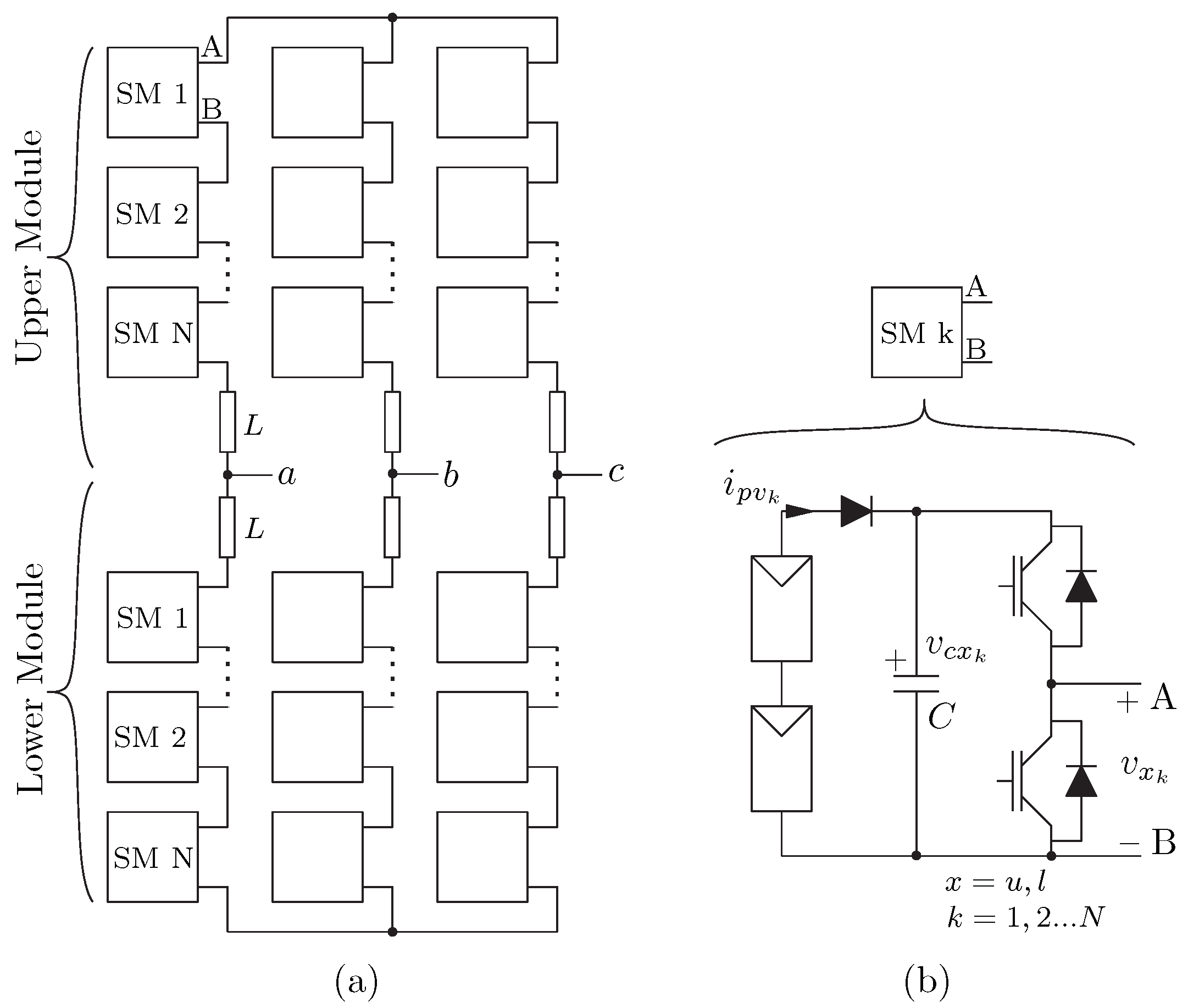
The modular multilevel converters meet these requirements and have gained much attention towards PV applications [5,6,7,8,9,10]. The multilevel inverter topology increases the MPPT granularity compared to central inverter and has very high efficiency compared to 2L/3L-inverters. Both the cascade H-bridge and the Modular Multilevel Converter (MMC) have similar efficiency profile. However, the main advantage of the MMC is that it increases the MPPT granularity by a factor of two compared to cascaded H-bridge for the same number of switching device. The MMC proposed in [11] is investigated in [10] for large scale PV plants, compared to other multilevel inverter topologies the MMC with half-bridge Sub-Module (SM) can be designed for maximum MPPT granularity with minimum number of switching devices. Furthermore, by using hybrid arrangement of the SMs the capacity to handle asymmetric power generation and DC fault can be improved [12,13]. The detailed discussion on average modeling the MMC is discussed in [14], the control methods are elaborately discussed in [15,16]. A distributed control scheme and approaches to specifically using PV panels in the SMs are discussed in [17,18]. The three-phase MMC with half-bridge SM is shown in Figure 1. The upper and lower arms of the MMC are series connection of the SMs, the variants of the SMs are discussed in [19]. Figure 1b shows the SM with Half-Bridge (HB) converter and the PV string connected directly to the SM capacitor with a series diode.
To use the modularity of the MMC, the PV strings are connected to the SMs. The variants of connecting the PV panels to the SM is discussed in [20]. The common method is to use a DC–DC converter as discussed in [10]. When the PV strings are grounded for safety, an isolated DC–DC converter is necessary as an interface between the PV string and the SM. The DC–DC converter decouples the MMC control and the MPPT control that is required for each of the PV string. The MMC control focuses on injecting power to the grid and maintaining a balanced operation of the MMC. The DC–DC converter control focuses on tracking the maximum power for the PV string in each of the SM. Due to the presence of additional DC–DC converter, SM voltage of the MMC need not be varied to track the maximum operating point for the PV string. Therefore, the MMC DC link voltage is fixed. The MMC can be designed for maximum efficiency at the desired DC link voltage. In this configuration, the overall efficiency decreases due to additional DC–DC converter, the capital cost also increases, and the overall reliability of the system decreases. In [21], the MMC-based PV plant is proposed with the PV string directly connected to each SM, thereby, eliminating the need for the DC–DC converter. In this topology, MPPT for the PV string in each of the SM must be integrated with the MMC control. The SM capacitor voltages must be varied to track the maximum operating point of the PV strings. In this configuration, there is no requirement for DC–DC converter, therefore, the overall efficiency and reliability of the system is high.
The control schemes proposed in [22,23,24] investigate the operation of the MMC as rectifier or inverter with energy source connected to the DC link. Such schemes are suitable when the PV string is connected to the DC link or to the SM using DC–DC converter. In [25], the control of the MMC is investigated with the energy source connected to the SM using a DC–DC converter and the DC link is assumed to be connected to a DC source. The control ensures balanced operation despite unbalanced power generation in each of the SM and delivers a balanced three-phase output power. In [21], the operation of the MMC is investigated when the PV string is connected directly to the SM without any DC–DC converter, this approach is based on the model predictive control proposed in [18]. The control ensures balanced output power between the phases of the MMC despite unbalanced power generation; however, the tradeoff is between the maximum power extracted from the PV strings. The coefficients in the model predictive control is chosen by trial and error to have a balanced operation and maximum power exaction from the PV panel. The basic concept in the control schemes present by [18,21], to balance the MMC when the energy source is connected to the SMs, is achieved by introducing a fundamental component of the circulating current–both positive and negative sequence. Based on the desired active power and minimization of power loss due to reactive power, mathematical expressions are presented for fundamental circulating current magnitude and phase. Such an elaborate control scheme for balanced operation of the MMC is necessary when the dynamics of the upper arm and lower arm are not considered separately.
In this paper, a novel control scheme in stationary frame is proposed for the MMC to extract maximum power from PV strings in each of the SM without the need for additional DC–DC converters and inject balanced power to the grid. The proposed method allows the control of power in each upper and lower arm individually and increases the MPPT granularity without need for additional hardware. A novel algorithm that tracks the SM capacitor voltages to their respective voltage references is proposed. The SMs in each arm of the MMC tracks a MPPT reference. The MPPT granularity in the proposed solution is increased to six instead of one in traditional central inverter. When the MMC is used as central inverter for the PV plant with each PV strings connected to the SMs, the connection to the DC link is not necessary. Therefore, the positive and negative terminals (‘p’ and ‘n’ in Figure 1a) of the MMC are left floating. The common mode voltage at these nodes provide additional degree of freedom for control of power flow. Therefore, the balance of power between the phases can be achieved by modifying the common mode voltages similar to that in star connected cascaded H-bridge converter [26]. However, the amount of power flow between the phases is controlled by controlling the DC component of the circulating current. The proposed scheme does not need sequence components to achieve balance operation as proposed in other control schemes for the MMC PV applications [18,21,25] and minimizes mathematical computation. The control scheme allows the MMC to be controlled as six independent generators such that power injected in phase are identical without any tradeoff on the MPPT for PV strings. A detailed analysis and simulation results are presented to validate the proposed control method and the tracking algorithm.
2. Modeling of MMC with PV String on Each SM
In the absence of DC link voltage, the per-phase model of the MMC derived in [16] needs to be modified to account for the common mode voltages. While deriving the average model for the MMC equal power distribution is assumed in both the upper arm and lower arm. However, when the PV strings are connected to each of the SMs in the MMC the power generation in upper arm and lower arm need not necessarily be equal due to unequal distribution of irradiance. A general model is necessary that accounts for unequal generation of power without any assumptions based on symmetry in operations.
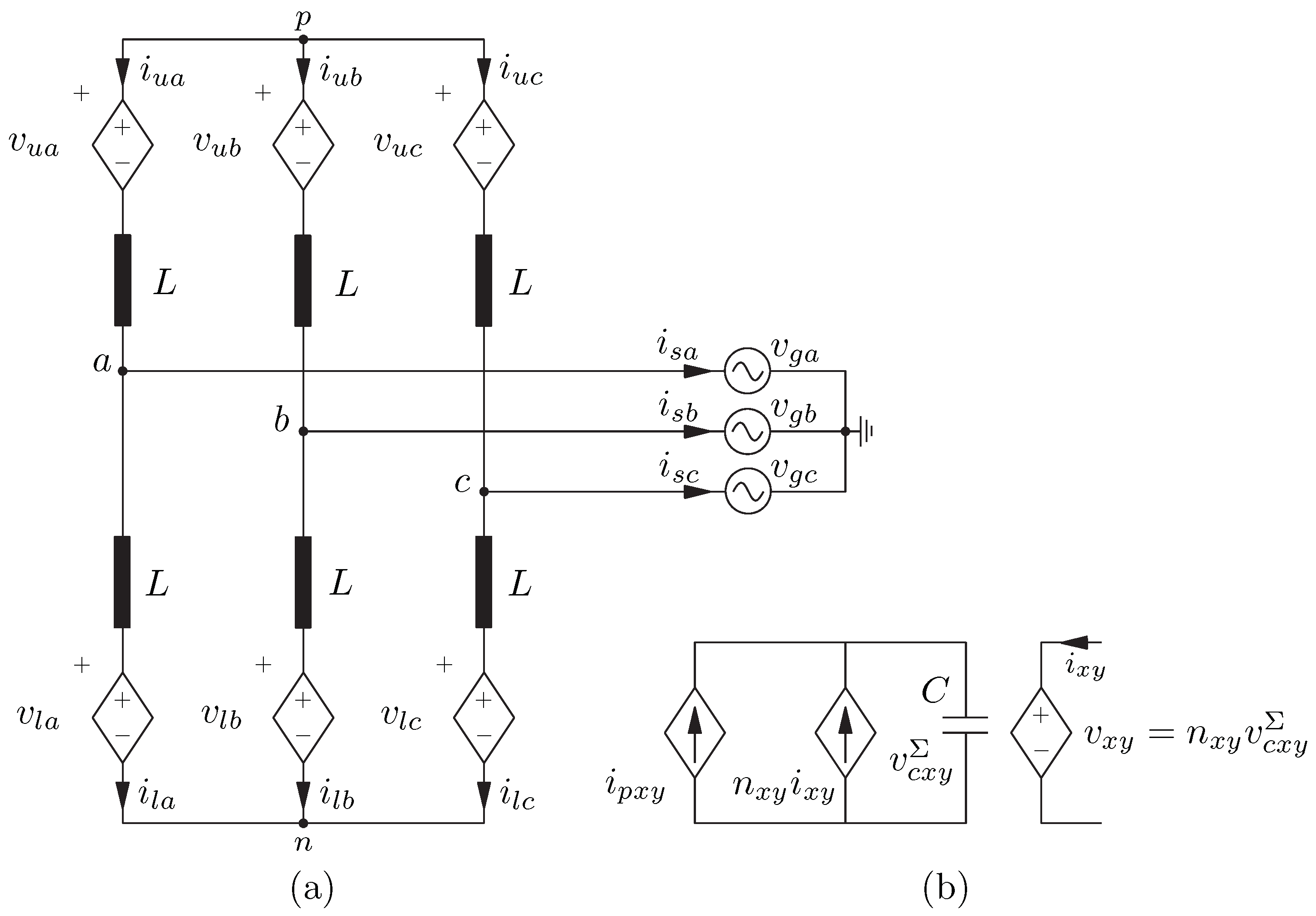
The MMC is made of upper and lower arms as shown in Figure 1a, the HB-SM structure is shown in Figure 1b. The PV string is directly connected to the SM capacitor; therefore, the DC link is not used. The HB-SM are identical in all the upper and lower arms in each phase. The arm inductance and ESR are identical in each arm. The equivalent model of the MMC is shown in Figure 2a with grid connection. The upper and lower arms are modeled as dependent voltage source which is a function of PV current, insertion index and arm current as indicated in Figure 2b. The common nodes ‘p’ and ‘n’ of upper and lower arms are left floating. The system is analyzed on a per phases basis, therefore, the subscript ‘y’ is dropped. The dynamic equations of the upper arm and lower arm currents are expressed as (1) and (2) considering the voltages at the output terminals of MMC.
The common mode voltages at node ‘p’ and ‘n’ regarding the ground (’g’) can be calculated using (1) and (2) for each phase as,
Subtracting (1) from (2) results in (5),
where the MMC output voltage is expressed as,
The output current is expressed as,
The imbalance voltage is defined as,
Unless a DC component is desired at the output voltage, must be forced to zero. The current that is common to both the upper and lower arms is referred to as circulating current. Therefore, each arm currents can be divided into two components: output current and circulating current.
The currents, , , are the contribution of the upper arm and the lower arm currents to the output current, . The circulating current, , flows through upper and lower arms and does not appear in the output current. It is equal in magnitude and phase, in both the upper and lower arms. However, for the MMC topology considered, it is not appropriate to define circulating current as average of the upper arm and the lower arm currents as the contribution of arm currents to the output current need not be equal. The arm currents do not have any DC current under balanced operation. However, the power between the legs of the MMC are redistributed using the DC component of the circulating current. The power between the arms of the MMC can be distributed using the fundamental component of the circulating current. Therefore, the circulating current has a DC, a fundamental, and another harmonic component. Among the other harmonics in circulating current within the MMC, the second harmonic current is dominant and is not desired. Therefore, the average value of the arm currents will equal to the DC component of the circulating current, .
The DC link voltage (potential difference between the nodes ‘p’ and ‘n’) is expressed as,
The inserted voltage for upper or lower arm is expressed as,
The insertion index is expressed as,
The dynamic of individual SM capacitor voltage is expressed as,
Assuming that the PV currents in each of the SMs are identical, all the SM capacitor voltages in the upper arm are equal to and all the lower arm SM capacitor voltages are equal to . The dynamics of sum capacitor voltage is obtained by summing the effects of individual capacitors in an arm of the MMC as,
The instantaneous power in each arm is expressed as,
The terms ‘’ is the collective power from the PV strings connected to an arm of the MMC. A general model of the MMC is described without imposing any restriction on operation.
3. Proposed Control Strategy
The objective of the control is to extract maximum power from the PV strings connected to each of the SMs and at the same time to deliver a balanced three-phase power to the utility grid. First, the requirement for the balanced operation is outlined and later the proposed arm power control for the MMC is discussed.
3.1. Requirement for Balanced Operation
The MMC is connected to the AC grid, this imposes restrictions on the operation of MMC as an inverter. It is required to maintain balanced sinusoidal voltages at the output of the MMC and inject balanced three-phase sinusoidal currents into the grid.
3.1.1. Constraint 1
The condition for balanced operation is expressed as,
From (18), the condition for upper and lower arm currents can be written as,
Since the common mode nodes ‘p’ and ‘n’ are left floating, the arm currents must sum up to zero. Assuming balanced grid voltages and using (19) the common mode voltages expressed in (3) and (4) are simplified as,
3.1.2. Constraint 2
Furthermore, for balanced operation at point of common coupling it is necessary that the power in each phase of the MMC is equal. However, it is not required that the PV power supplied to the grid from the upper and the lower arm is equal. When the PV power produced in each phase is not equal, the PV power produced above the average value in each phase needs to be distributed to other phases.
3.1.3. Constraint 3
The average value of the output voltages of MMC over the fundamental period must be zero () to avoid injection of DC currents into grid. Using (5) this constraint is expressed as,
From (22), it can be stated that in order not to have a DC offset at the output voltage the deviation of average voltage of the upper and lower arm from their common mode voltage at node ‘p’ and ‘n’ should be zero.
3.2. Proposed Arm Power Control of MMC
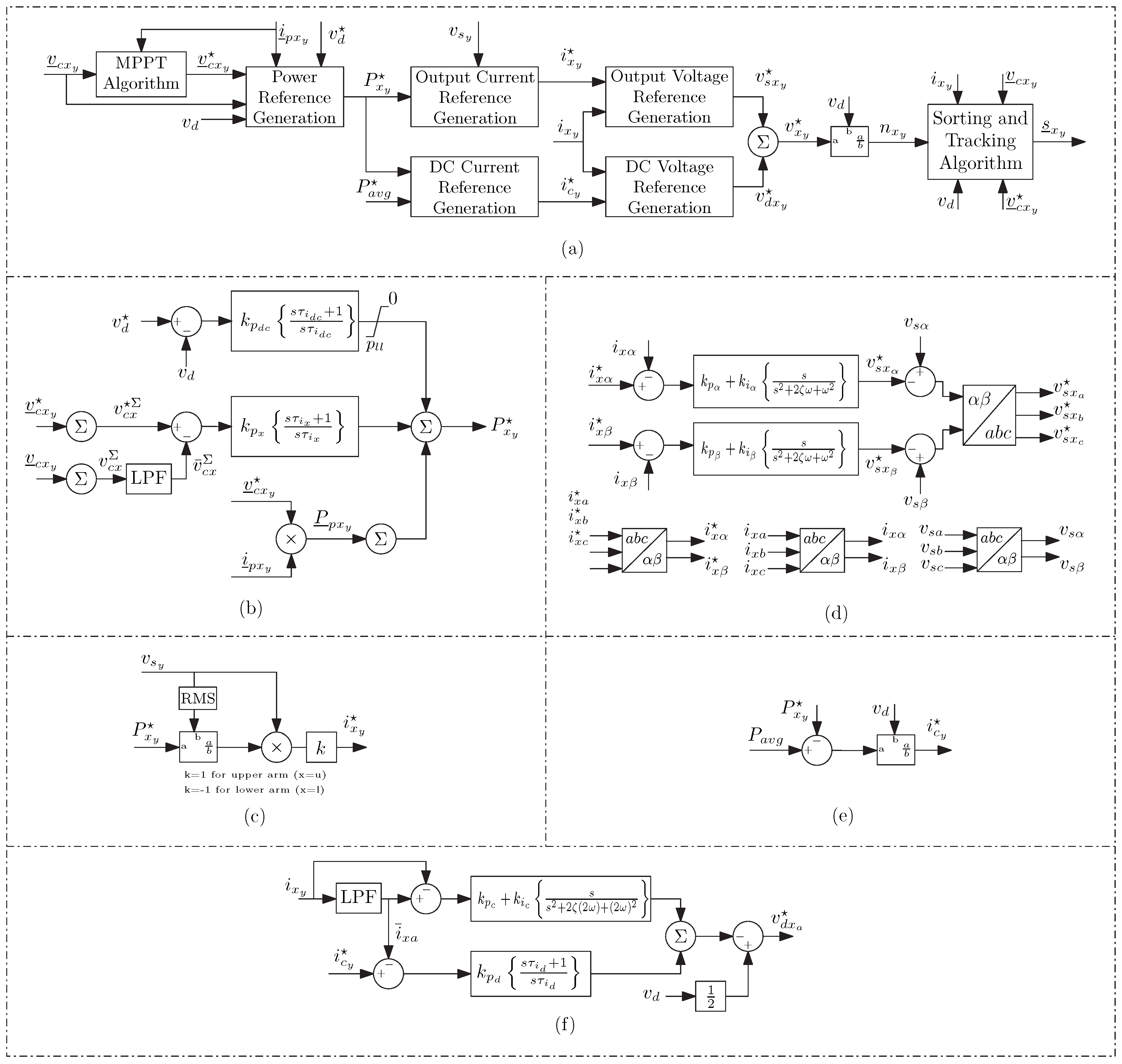
The proposed arm power control scheme for each arm of the MMC is shown in Figure 3a. The arm inserted voltage reference for upper or lower arm of the MMC is obtained separately based on the PV power produced by each arm. It is equal to the sum of voltage reference from the output current controller and the circulating current controller as,
The insertion index for each individual arm is obtained as,
In this section, the control blocks shown in Figure 3 are described in detail.
3.2.1. MPPT Algorithm
The MPPT algorithm tracks the maximum power point for the PV strings connected to the SM. The voltage reference from the MPPT controller is a row vector with SM capacitor voltage references for individual SM in an arm of the MMC. The SM capacitor voltage reference row vector, , is provided to the voltage-tracking algorithm. The same reference is also provided to the power generation block to regulate the power delivered to the grid from the respective arm of the MMC. The proposed tracking algorithm makes sure that the SM capacitor voltages are at the reference voltage as requested by the MPPT algorithm. Therefore, the tracking algorithm acts as innermost control loop. The SM capacitor voltages are dynamically altered with the help of tracking algorithm. Traditional MPPT methods [27] that require altering the PV string terminal voltage to track the maximum operating point can be used, thereby avoiding the need for complex MPPT algorithm based on advanced control methods.
3.2.2. Power Reference Generation
The power reference generation is shown in Figure 3b. The reference is the feed-forward term obtained by summing the power generated by each PV strings in an arm of the MMC. The voltage limit is provided to protect the SM capacitor from charging beyond the maximum DC link voltage, under normal operation this loop is not operational. The power reference is regulated by controlling the sum of the capacitor voltage, , for a given arm. The MPPT voltage reference for each SM in an arm of the MMC is added to generate a sum capacitor voltage reference . Therefore, the power reference is expressed as,
is the desired power contribution by the arm to the AC grid.
3.2.3. Output Current Reference Generation
The active current definition presented in the time-domain Conservative Power Theory [28,29], is used to obtain the output current reference. Figure 3c shows the output current reference obtained from the active power reference and for an arm of the MMC. This is mathematically expressed as,
The output reactive power is set to zero, therefore, the reactive current reference is zero. Each phase has two current references, one for the upper arm and the other for the lower arm of the MMC.
3.2.4. Output Current Controller
Figure 3d shows the realization of the output current controller. For (18) to be true, the output current should not have any common mode current. To avoid the common mode component in the output current reference, a common mode filter can be realized by simply transforming all the upper arm and lower arm reference currents into -stationary frame. PR controller is used in the stationary frame to generate the required AC voltage reference for the upper and lower arms. By using -stationary frame the number of PR controllers required is also reduced. The transformed reference current is expressed as,
The measured upper arm currents and lower arm currents in the three phases of the MMC are also transformed similar to (27). The three measured phase output voltages are also transformed to -stationary frame as , respectively. The AC voltage reference for the upper or lower arms for three-phase MMC expressed is expressed in -stationary frame as,
The per-phase upper arm or lower arm output voltage references are obtained as,
3.2.5. DC Circulating Current Reference Generation
The DC link (node ‘p’ and ‘n’) of the MMC is not used, as a result there is no exchange of power between the DC link and the grid. Therefore, the DC link current in general is zero. In the normal operation, i.e., equal irradiance level in each arm, each leg of the MMC is generating equal power. Therefore, there is no need for transferring power between the legs of the MMC. In this case, the average value of the arm current is zero. However, in case of unequal irradiance on each arm of the MMC the power produced in each phase will not be equal, this is not desired as it leads to unbalanced current injection into the grid. For unequal power generation in each phase there is a need to transfer power between the legs of the MMC to inject balanced active power into grid and to avoid unbalance in the output currents. This transfer of power between the MMC legs is achieved by controlling the average value of the arm current. The power generated from the PV strings in each arm is expressed as,
Then the average power per arm is expressed as,
In case of equal irradiance, the power generated by each arm of the MMC is equal to the average value of power per arm of the MMC, i.e., . When all the SM capacitor voltages are equal to their mean value, then (16) can be written as,
To avoid increase or decrease the stored energy in the SM capacitor voltage i.e., to maintain the desired MPPT voltage reference, the average change in arm stored energy over a fundamental period should be zero, . Representing the voltage and current in terms of their average and AC values, (32) simplifies to,
Considering the average value of (33) leads to,
In normal operating conditions, , therefore, . However, when , the desired power injected to the grid from each arm of the MMC to avoid unbalance is,
The difference between (34) and (35) gives the reference for the desired DC current in the arm in order to either transfer power to (or receive power from) other legs of the MMC so the power injected to the grid from that particular arm is equal to . This is expressed as,
Figure 3e shows the generation of DC circulation reference for each arm of the MMC. To avoid DC current injection to the grid, the desired average value of the arm currents in a leg of the MMC must be equal, . Summing the condition stated in (36) for upper and lower arm, DC circulating current reference for each arm of the MMC is expressed as,
From (19) it is seen that . The desired average value of the inserted arm voltage is . Therefore, (37) is simplified as,
It is possible to use the proposed control for other applications requiring DC link, such as HVDC transmission. In such applications, the control scheme needs additional DC circulating current reference to handle the power flow from the DC terminal. If the total power from (or injected to) the DC link is , then the additional DC circulating current reference added to (38) will .
3.2.6. Circulating Current Control
Figure 3f shows the realization of circulating current control. A PI controller is used to track the DC current reference on each arm of the MMC. This ensures that the required power is either transferred from the leg or received from other legs of the MMC. Furthermore it also ensures that the average values of upper and lower arm currents are equal and no DC current is injected to the grid. The arm current has circulating harmonic current other than the fundamental current, and the dominant component begins the second harmonic current [14]. It is desired not to have any harmonic current component other than the DC and fundamental in arm current. Therefore, a PR controller is used to suppress the second harmonic circulating current [30]. The DC voltage reference for the arm of the MMC is obtained as,
is the voltage reference from the second harmonic circulating current suppressor for an arm of the MMC.
3.2.7. SM Capacitor Voltage-Tracking Algorithm
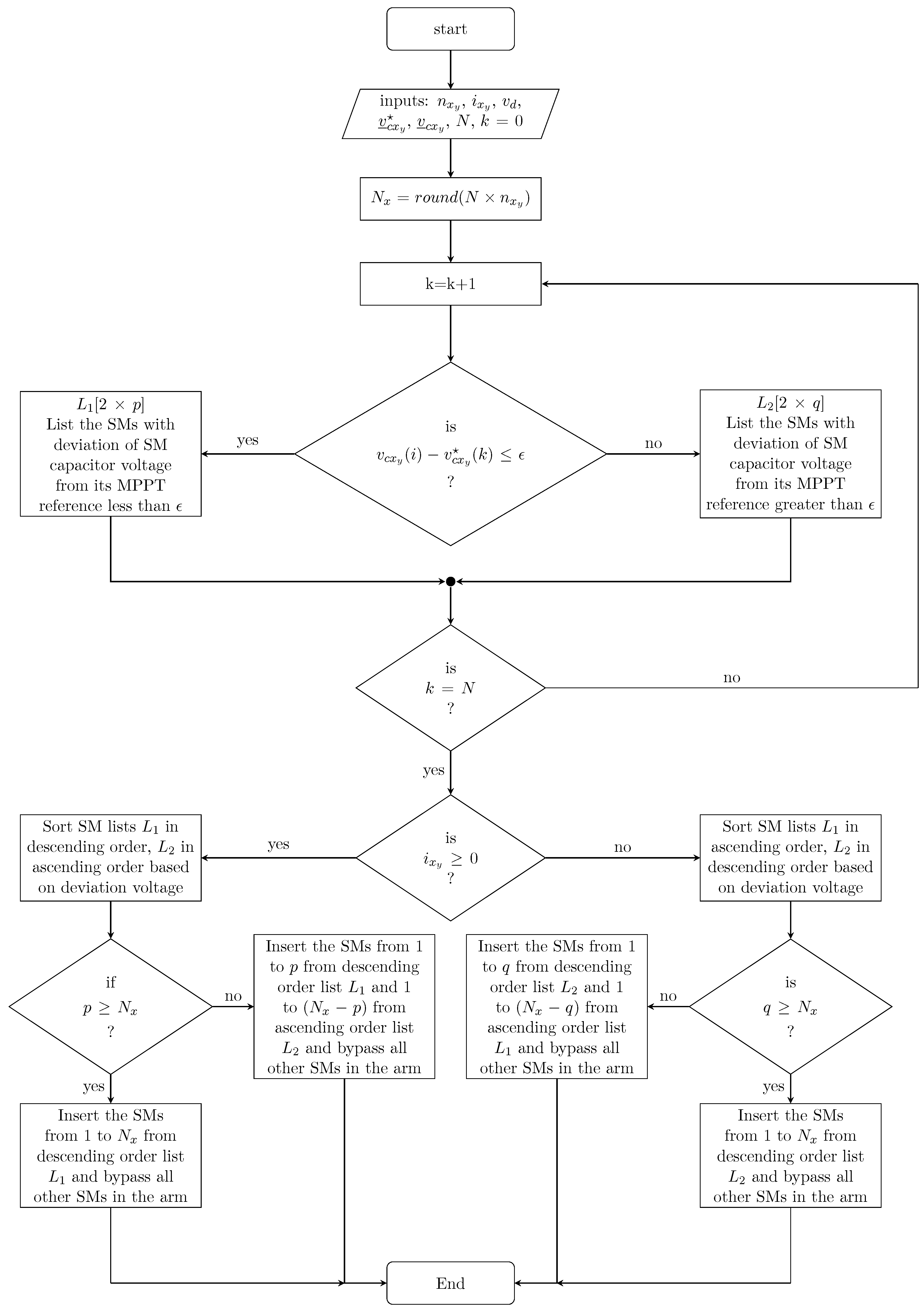
A novel SM capacitor voltage-tracking algorithm is proposed, which allows the SM capacitor voltages in an arm of the MMC to be maintained at desired individual MPPT voltage references for each of the SM. The proposed reference tracking algorithm along with nearest level control modulation scheme [31] is shown in Figure 4.
The voltage reference for each SM capacitor in an arm of the MMC is provided by the MPPT algorithm. The number of SMs to be inserted for a given arm is rounded off to the nearest integer.
Two separate lists, and , are prepared depending on the deviation of SM capacitor voltage from the desired reference. The list is a row vector, registering all the SMs and their respective capacitor voltage deviation from reference less than . The list is a row vector, registering all the SMs and their respective capacitor voltage deviation from reference greater than . Where is the allowed voltage threshold, if this hysteresis is not desired then is set to zero. Depending on the direction of the arm current, the voltage deviations in the lists and and the associated SMs are sorted in ascending or descending order, as shown in the flow chart. When and , the required number of SMs, , is inserted from the descending order list and all other SMs in an arm of the MMC are bypassed. When and , all the SMs in the descending order list is inserted and remaining () SMs from the ascending order list are inserted, all other SMs in an arm of the MMC are bypassed. Similarly, when and , the number of SMs to be inserted, , is selected from the descending order list and all other SM in the arm are bypassed. When and , all the SMs in the descending order list is inserted and remaining () SMs from the ascending order list are selected, all other SMs in an arm of the MMC are bypassed. The proposed tracking algorithm minimizes the deviation from the MPPT voltage reference for each individual SM capacitor voltages.
3.3. Requirements on Current and Voltage Measurement
The proposed control method uses closed loop control. It requires six current sensors to measure the arm currents and ‘’ SM capacitor voltage measurements. In control schemes proposed in [7] referred as open loop control of the MMC, the ripple on the sum capacitor voltage is estimated and the DC link voltage is directly measured. This scheme needs only one voltage measurement on the DC link. In other widely used MMC control scheme proposed in [15], ‘’ SM capacitor voltage measurements are necessary. In all control methods where the energy source is connected to each of the SM, the capacitor voltage measurement is necessary. The grid side voltages are also measured, therefore, a total of ‘’ isolated voltage measurements are necessary.
If PV string currents are measured, then a total of ‘’ current sensors are necessary. In the proposed control method, a direct measurement of PV current is not necessary. The total power injected to the grid from the arm gives an indirect estimate on power harvested from PV strings. The MPPT algorithm uses the power injected from the arm to the MMC to the AC grid to calculate the SM capacitor voltage reference. This avoids the need for additional ‘’ current sensors.
4. Simulation Results
A model of the MMC is developed as shown in Figure 1 in MathWorks Simulink. The switching model for the SM is chosen. The PV string is modeled as a current source that depends on irradiance and SM capacitor voltage. The simulation model is used to verify the proposed control method along with the voltage-tracking algorithm. Table 1 summarizes all the parameters of the MMC used in this simulation. It should be noted that the capacitance in each SM is 20 mF; however, the maximum capacitor voltage is 75 V. Therefore, an electrolytic capacitor can be used with reduced dimension unlike the case in HVDC applications. The data for PV panel is obtained from Canadian Solar CS6K-285M-FG with maximum system voltage of 1500 V [32], two of such panels are connected in series to form a PV string. The controller parameters are tabulated in Table 2. The outer control loop has high bandwidth approximately 1/10th of the switching frequency. For this simulation, the power reference generation control has a higher bandwidth than the average circulating current controller. The control parameters, chosen for this simulation study, are tuned aggressively. However, in practical system, since the irradiance change is not drastic, the power reference generation control can be tuned with lower bandwidth comparable to that of average circulating current controller.
The power flow under three different irradiance cases are discussed. In the first case, the lower arm in all the phases produce equal power and very low power is generated from upper arms of the MMC. This situation shows the independent power injection from the upper and lower arms in the MMC. In the second case, one of the upper arms and two lower arms produce equal power and very low power is generated in other arms of the MMC. In this situation, each phase produces equal power, it is shown that currents circulate in the MMC to maintain the desired balanced output power without any need for power transfer between the legs of the MMC. In the third case, only one upper arm of the MMC produces power. This is an extreme unbalanced power generation where other five arms of the MMC produce very low power. It is shown in [15] that the circulating current flows within the MMC, the DC component of the circulating current transfers power from one phase to the other and a balanced output power is injected to the grid. In all these cases, the voltage-tracking algorithm maintains the SM capacitor voltage at a MPPT voltage reference to extract maximum available power from the PV strings connected to each of the SMs without interfering with the operation of the MMC.
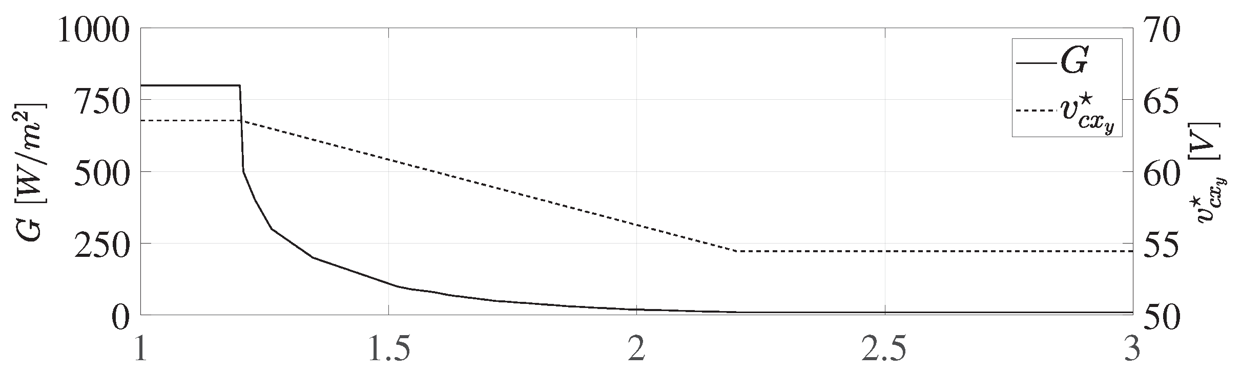
In each of the cases, the standard rated condition is referred to as normal condition, i.e., at irradiance of 800 W/m, spectrum AM 1.5, ambient temperature 20 °C, wind speed 1 m/s. Each arm injects around 8.7 kW of power to the grid. To simulate the shaded condition, the MPPT reference is linearly decreased from 63.54 V to 54.46 V over a period of 1 s. The irradiance is also decreased as a function of MPPT voltage reference that decreases from 800 W/m to 10 W/m in this duration. The PV current changes as a function of MPPT voltage reference and irradiance from 7.2120 A to 0.0898 A. The shaded arm of the MMC injects around 100 W to the grid. The variation of irradiance for shaded condition is shown in Figure 5. Furthermore, it is assumed that the SMs in the affected arm of the MMC is uniformly shaded. The normal condition is maintained until t = 1.2 s and the shaded condition is applied from t = 1.2 s onwards for all the cases.
4.1. Case 1: The Upper Arms of the MMC Does Not Generate Power
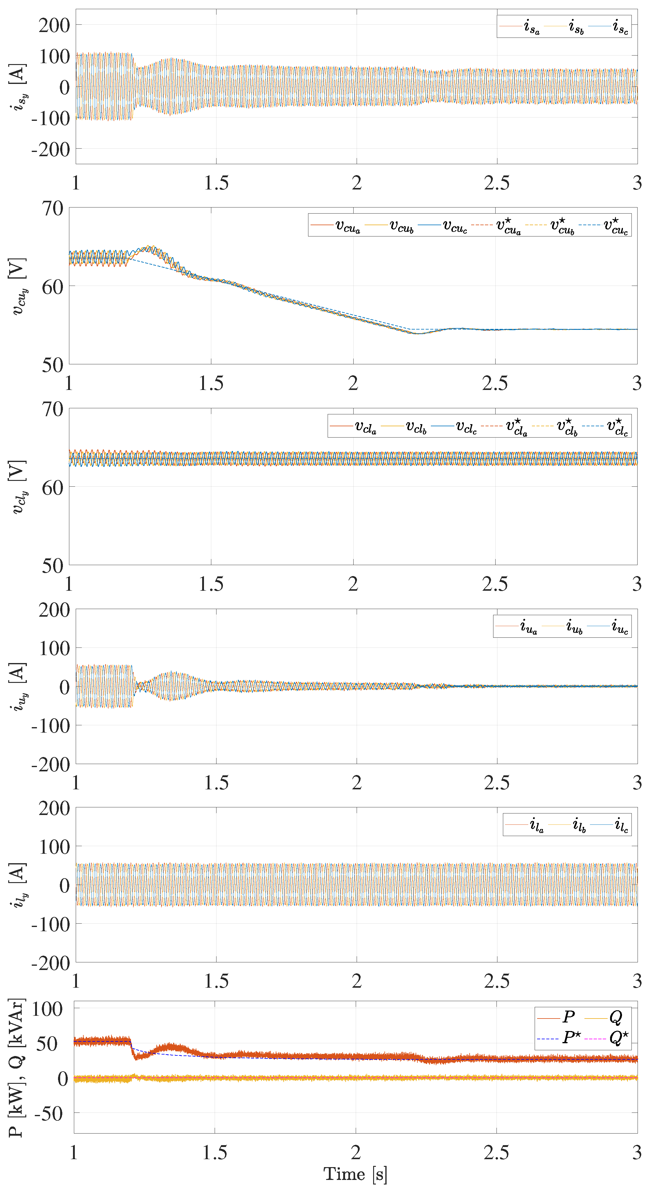
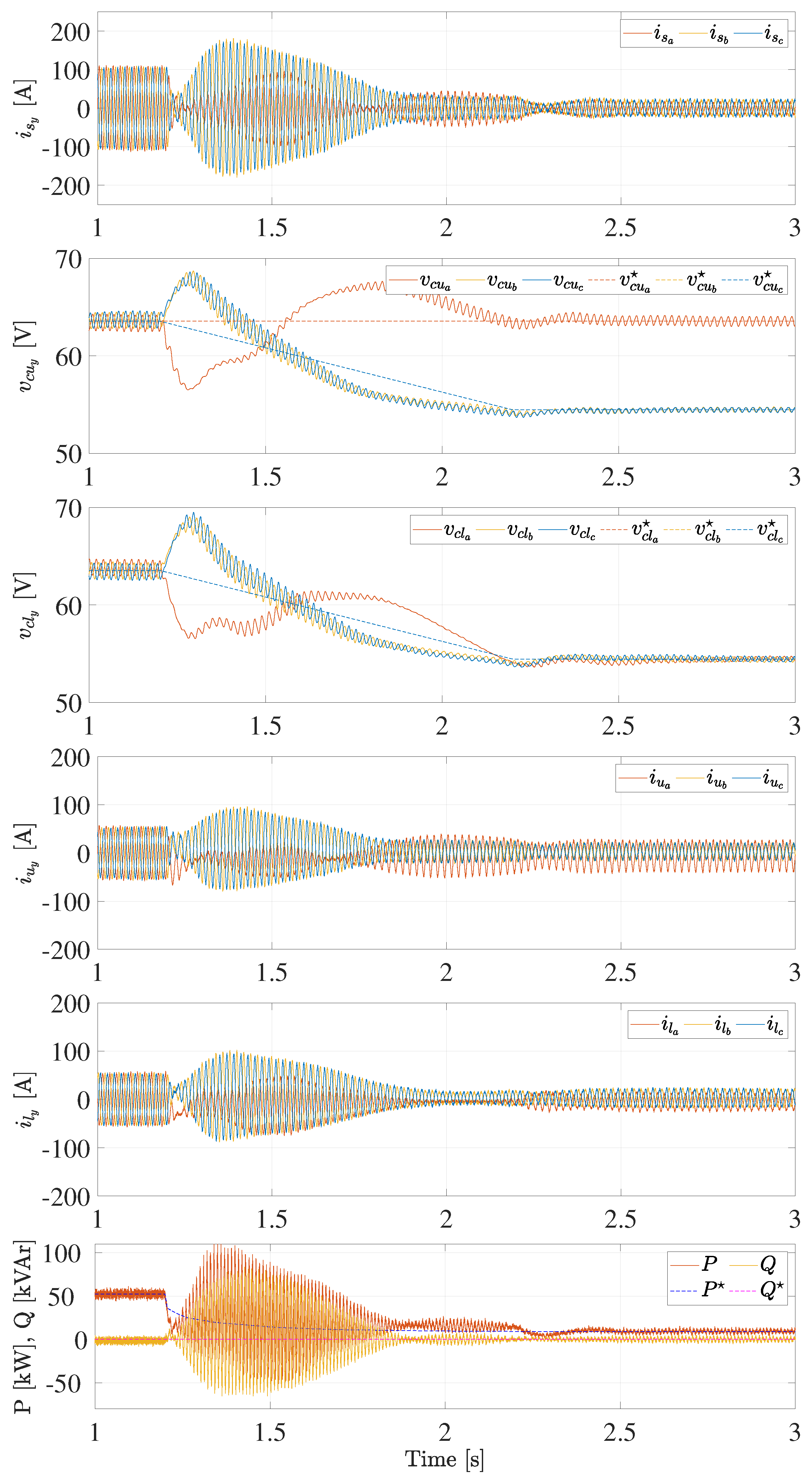
In this scenario normal irradiance is assumed on all the lower arm SMs and shaded condition on all the upper arm SMs. The total power production reduces to one third of the power generated under normal operation. The results are shown in Figure 6, until t = 1.2 s the MMC converter injects balanced power to the grid. The output voltage and output current are balanced and the MMC injects 52.26 kW of active power (P) to the AC grid. The SM capacitor voltages are balanced, and are maintained at the MPPT voltage reference of 63.5 V for irradiance level of 800 W/m. At t = 1.2 s, the shaded condition is applied to all the upper arms of the MMC, the irradiance is decreased to 10 W/m in 1 s. The MPPT voltage reference for the upper arm SMs is reduced to 54.46 V. The SMs in the upper arm track the MPPT voltage reference and the upper arm currents in all the phases decreases with each upper arm contributing 157 W to the AC grid. Meanwhile, the lower arm SM capacitor voltages, , are maintained at their respective MPPT references and the lower arm currents are not affected. The entire output current is dominantly contributed by the lower arm of the MMC, i.e., . The total power injected (P) to the grid is reduced to 26.4 kW and the reactive power (Q) is maintained to zero. The proposed control system enables the upper arms and lower arms to independently inject power to grid. The voltage-tracking algorithm enables extraction of maximum power from the PV string connected to each of the SMs without interfering with the inverter operation of the MMC.
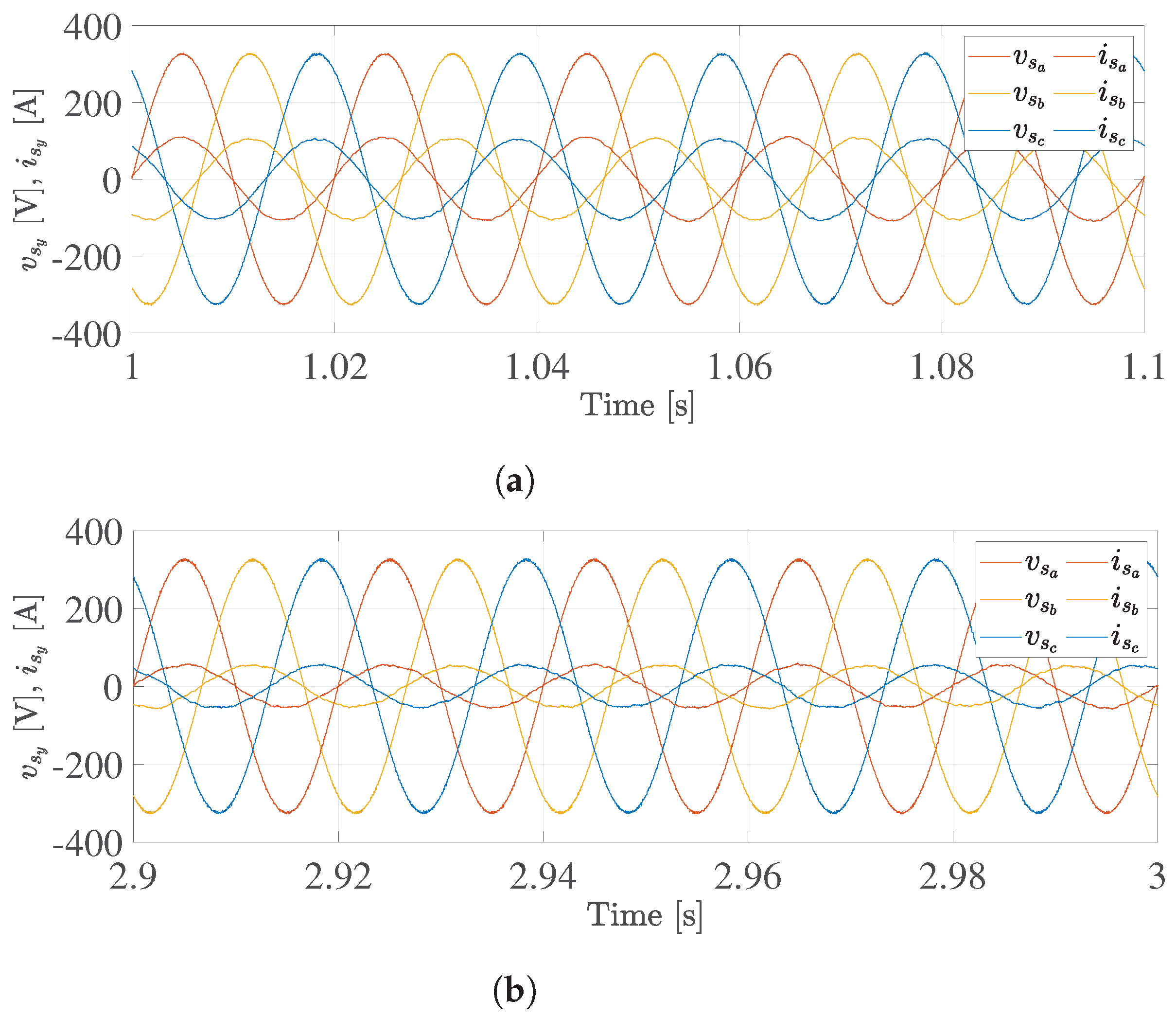
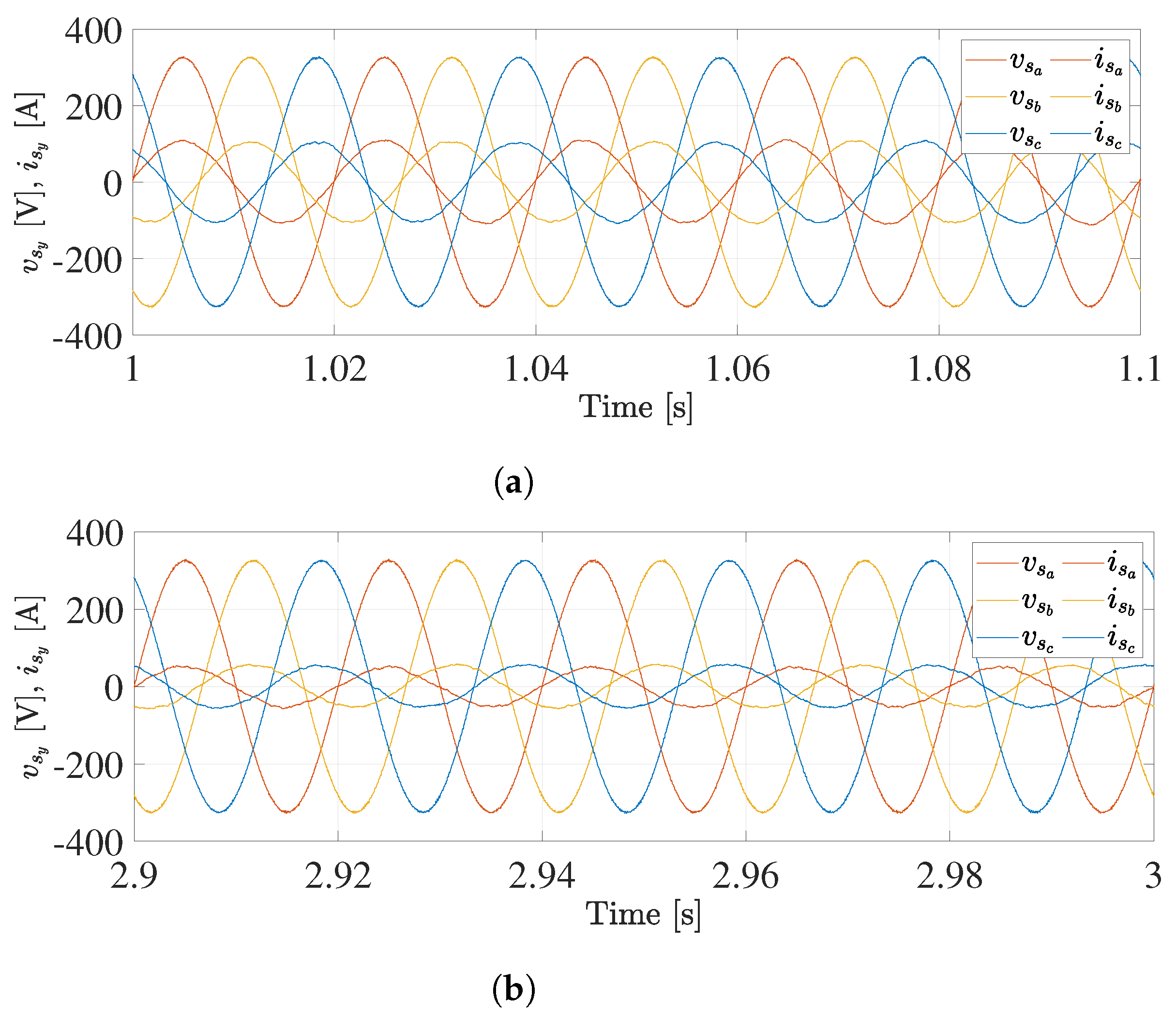
The three-phase grid voltages at PCC and output currents are shown in Figure 7a,b for a duration of 100 ms. From t = 1 s to 1.1 s the balanced voltages and currents are shown for normal operating condition. The output current is in phase with the respective phase voltage. In the shaded condition after the transients settle, from t = 2.9 s to 3 s, a balanced power is delivered with currents in phase with the voltages.
4.2. Case 2: One Lower Arm and Two Upper Arm of the MMC Does Not Generate Power
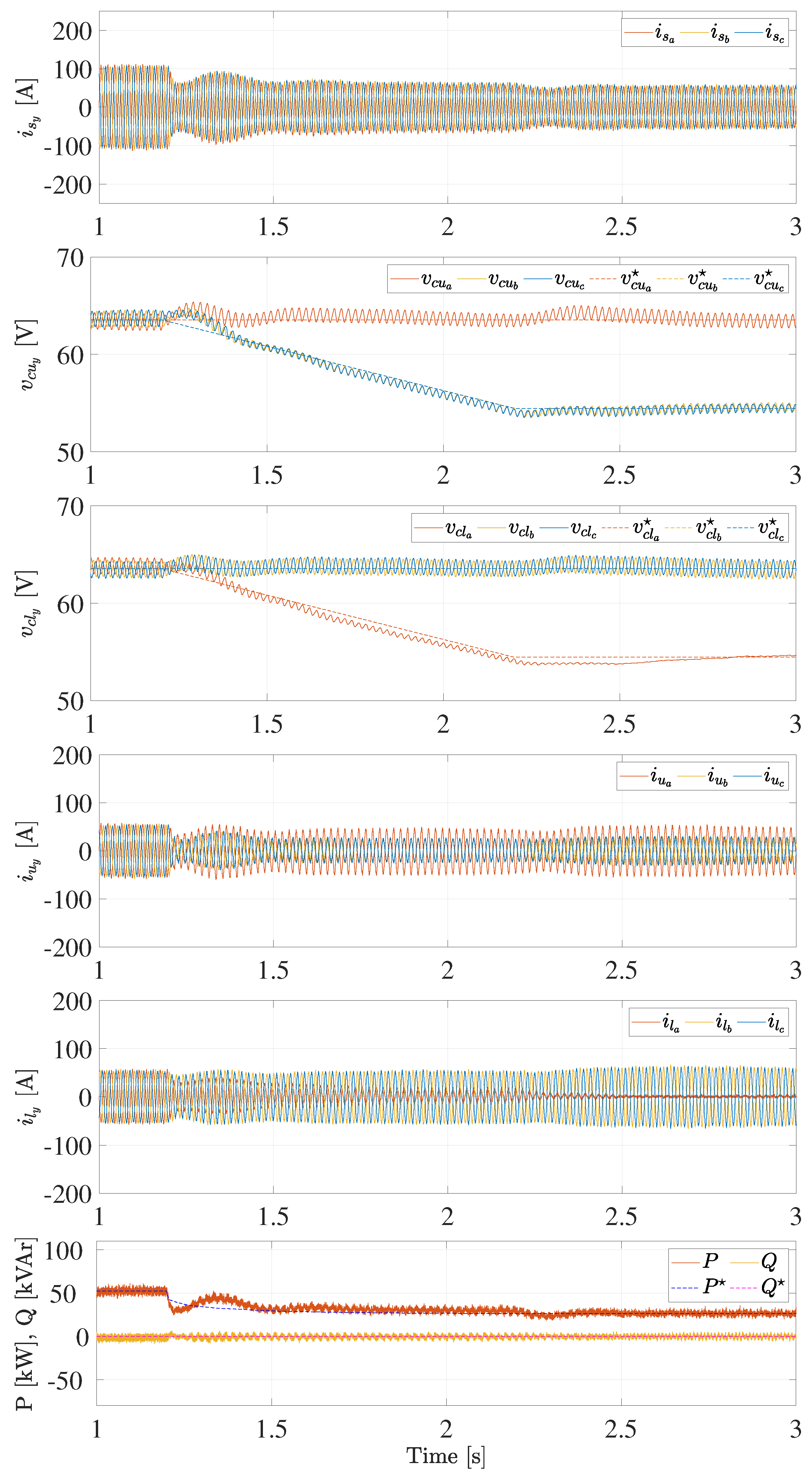
In this scenario shaded condition is assumed in phase ‘a’ lower arm and phase ‘b’ and ‘c’ upper arms of the MMC, respectively. The total power production in shaded condition reduces to one third of the power generated under normal operation. The results are shown in Figure 8, until t = 1.2 s the MMC converter injects balanced power to the grid. At t = 1.2 s, the shaded condition is applied, the SM capacitor voltages in phase ‘a’ upper arm and phase ‘b’ and ‘c’ lower arm does not deviate from its MPPT voltage references; however, phase ‘a’ lower arm and phase ‘b’ and ‘c’ upper arm SM capacitors have a new MPPT voltage references due to decrease in irradiance from 800 W/m to 10 W/m. It is seen that all the SMs track the voltage reference. Phase ‘a’ upper arm injects power into AC grid; however, phase ‘b’ and ‘c’ upper arm currents and the lower arm currents flow such that (19) is satisfied. This fundamental current in phase ‘b’ and ‘c’ upper arm does not contribute to the power to the AC grid, it circulates within the MMC. However, the DC component of the circulating current is zero, implying no transfer of energy from one phase to the others in the MMC. Furthermore, a balanced output current is injected into grid in phase with the grid voltage. As the SMs track the MPPT voltage reference the voltage also changes. The insertion index computed for each arm of the MMC is compensated by the outer current loop to account for variation in , thereby maintaining zero residual output voltage i.e., . The reduction is active power injected to the grid and the reactive power is also shown.
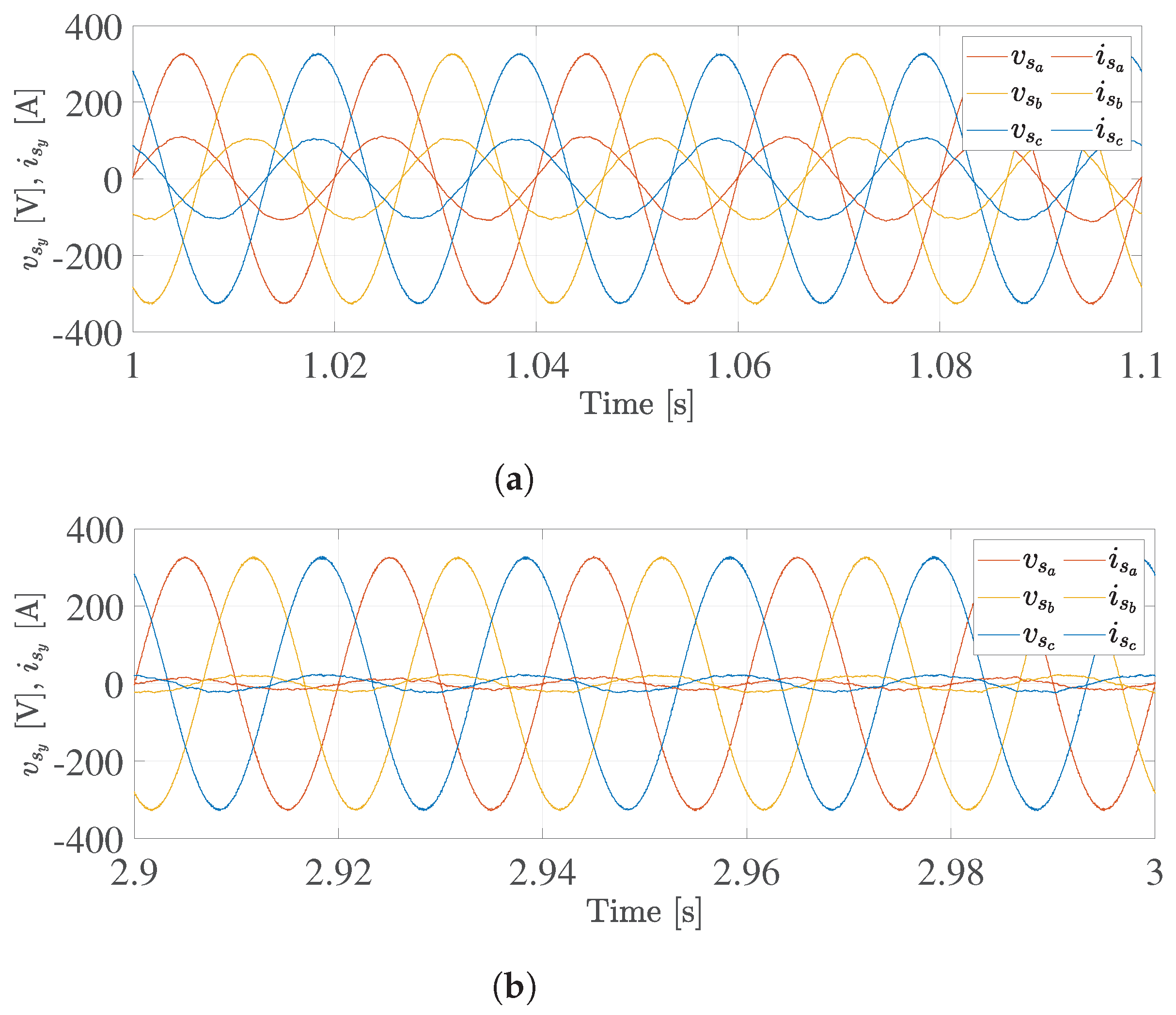
The three-phase grid voltages at PCC and output currents are shown in Figure 9a,b for a duration of 100 ms. From t = 1 s to 1.1 s the balanced voltages and currents are shown for normal operating condition. The output current is in phase with the respective phase voltage. In the shaded condition after the transients settle, from t = 2.9 s to 3 s, a balanced power is delivered with currents in phase with the voltages.
4.3. Case 3: One Upper Arm Alone Generate Power in the MMC
This is an extreme case where only phase ‘a’ upper arm receives an irradiance of 800 W/m and all other arms of the MMC are assumed to be shaded. The total power production reduces to one sixth of the power generated under normal operation. The results are shown in Figure 10, the shaded condition is applied at t = 1.2 s. The irradiance in all the SMs except the ones in phase ‘a’ upper arm is decreased from 800 W/m to 10 W/m. The SM capacitor voltages and in each leg of the MMC track the desired MPPT voltage reference. However, during transients a power oscillation is observed. This is due to the power exchange between the legs of the MMC and the power injection from each phase of the MMC to the grid. The power oscillations are damped in 1 s. The controllers can be tune less aggressively by having a longer settling time to reduce the magnitude of the power oscillation between the grid and the MMC. The fundamental circulating currents flow within the MMC to maintain the condition stated in (19). To inject balanced power into the grid, DC circulating current flows from phase ‘a’ leg of the MMC to the phase ‘b’ and ‘c’ legs of the MMC respectively, this flow of DC current is regulated by the PI controller in the circulating current control. Even with such extreme unbalanced power generation, the MMC can inject a balanced output current into grid, in phase with the grid voltage. The active and reactive powers injected into the grid are also shown.
The three-phase grid voltages at PCC and output currents are shown in Figure 11a,b for a duration of 100 ms. From t = 1 s to 1.1 s the balanced voltages and currents are shown for normal operating condition. The output current is in phase with the respective phase voltage. In the shaded condition after the transients settle, from t = 2.9 s to 3 s, a balanced power is delivered with currents in phase with the voltages.
4.4. Observations and Discussions
For all the three extreme cases presented the MMC can harvest the maximum available power from the PV strings and inject balanced power to the grid at unity power factor. In case 1 the only lower arms of the MMC contributes active power. There is no need for energy transfer from lower arm to upper arm in a leg of the MMC. Therefore, additional circulating currents are not necessary. In case 2, voltage reference for arms are generated such that the constrain expressed in (19) is obeyed. In case 3, the DC circulating current reference as well as the fundamental circulating current reference are used to move the power between the legs of the MMC and between the arms in each leg of the MMC. Mathematical computation of reference for fundamental circulating current is not necessary in either of the cases. This is will not be the case when fundamental positive and negative sequence circulating components are used for balancing energy between the arms of the MMC [21] leading to additional power loss.
In all the cases discussed, it is seen that for the decrease in MPPT voltage reference from 63.54 V to 54.46 V as a ramp with slope of 9.08 V/s the SM capacitor voltages track their respective MPPT voltage references within 1.5 s. During the extreme unbalance in power generation, the power oscillations in the transients are effectively damped within 1 s and a balanced power is injected to the grid without compromising the extraction of the maximum power from the unshaded PV strings.
The model for the MMC developed assumes that there is no DC source connected between the node ‘p’ and ‘n’ respectively. The model will not be effective when a DC source is connected to nodes ‘p’ and ‘n’. In such cases the voltage can to be replaced with DC link voltage ‘’ to use the same control scheme presented. In comparison to other control schemes, the proposed method acts on individual arm and needs three additional circulating current controllers (refer Figure 3f) and at least three additional output reference generators (refer Figure 3d). The flexibility in control comes at increase in number of controllers. However, from an implementation perspective, these are identical control units that can be pipelined without increasing the burden on use area in FPGA or Processors. A delay in computation of ‘’ is not desired, the number of multiplication increases with number of SMs in the MMC. Therefore, calculation of ‘’ can be implemented in hardware such as FPGA or physical layer of System on Chip.
The MMC configuration used in the solution uses higher number of switching devices and capacitors compared to conventional 2L/3L-central PV inverters. This results in higher capital expenditure (CAPEX) of the MMC compared to the central inverter. The operational expenditure (OPEX) for the MMC is lower than the central inverter due to its modularity, the faulty SMs can be bypassed or hot swapped without hindering the operation of the MMC until the next maintenance cycle. Therefore, despite higher capital cost, the total life cycle cost would be comparable to central inverter. The advantage for the MMC is the increased MPPT granularity and with the proposed control the capability to extract available maximum power from single PV string to full installation of PV units. This results in much higher annual energy yield compared to central inverter. For the entire life cycle of the PV plant the energy yield would also be much higher in case of the MMC. Therefore, the levelized cost of energy defined as ratio of total energy yield to total cost over the life cycle of the PV plant will be lower for the MMC compared to the central inverter.
5. Conclusions
The paper proposes an arm-level control method for the MMC with the PV strings directly interfaced to the SMs. A voltage-tracking algorithm is proposed that enables the tracking of the maximum power in each of the PV strings connected to the SMs without the need for additional DC–DC converters. A detailed model of the MMC using common mode voltages is discussed, and the constraints for balanced operation of the MMC for arm-level power control are presented. The proposed control method is validated using simulations, and the proposed solution allows a balanced injection of power into the AC grid irrespective of the unbalance in the power generation in the MMC due to unequal irradiance. Furthermore, the voltage-tracking algorithm enables the extraction of the maximum power from each of the SMs even under the extreme unbalance in power generation.
The proposed solution is demonstrated for PV applications; however, it can be applied to other applications where the renewable energy source is directly integrated to the SMs. In all the cases discussed, it is seen that for the decrease in MPPT voltage reference from 63.54 V to 54.46 V as a ramp with slope of 9.08 V/s the SM capacitor voltages track their respective MPPT voltage references within 1.5 s. During the extreme unbalance in power generation, the power oscillations in the transients are effectively damped within 1 s and a balanced power is injected to the grid without compromising the extraction of the maximum power from the unshaded PV strings.
The proposed control method for the MMC with PV strings in each of the SMs increases the MPPT granularity. The proposed solutions do not need additional DC–DC converters; therefore, it avoids additional investments and leads to overall high efficiency. The high efficiency of the MMC and the MPPT tracking on individual SMs will increase the annual energy yield compared to classical central inverter.
The proposed control method is effective in handling unbalanced power generation in the MMC when the PV strings are directly integrated to the SM. The control scheme opens the possibility of exploring the PV system with storage by integrating batteries directly in a few of the SMs to perform auxiliary services required for grid services.
Author Contributions
Conceptualization, A.B.A., M.R., D.S., R.T. and L.E.N.; Formal analysis, A.B.A.; Investigation, A.B.A., D.S. and L.E.N.; Methodology, A.B.A. and M.R.; Resources, D.S. and R.T.; Supervision, D.S., R.T. and L.E.N.; Validation, M.R.; Writing—original draft, A.B.A.; Writing—review & editing, A.B.A., M.R., D.S., R.T. and L.E.N.
Funding
This research received no external funding. The APC was funded by NTNU Publishing Fund. We gratefully acknowledge financial support from the Department of Electrical Engineering, Norwegian University of Science and Technology.
Conflicts of Interest
The authors declare no conflict of interest.
Nomenclature
| Average value of ‘a’ over the fundamental period | |
| AC variable with zero average value | |
| RMS value of ‘a’ over fundamental period | |
| Row vector with dimension | |
| Upper (u) or Lower (l) arm | |
| Phase a, b or c | |
| Sub-Module index | |
| g | Reference ground |
| N | Number of Sub-Modules |
| Insertion index of kth Sub-Module in upper or lower arm per phase | |
| Insertion index of upper or lower arm per phase | |
| Upper or lower arm current per phase | |
| Output current per phase | |
| Circulating current per phase | |
| PV string current in kth Sub-Module per phase | |
| Capacitor voltage of kth Sub-Module in upper or lower arm per phase | |
| Sum capacitor voltage of upper or lower arm per phase | |
| Inserted upper or lower arm voltage per phase | |
| Output voltage in each phase | |
| Average arm capacitor voltage per phase | |
| Grid voltage per phase | |
| Common mode voltage at node ‘p’ | |
| Common mode voltage at node ‘n’ | |
| Effective DC link voltage | |
| Stored energy per arm in each phase | |
| Stored energy in each phase | |
| P | Three phase active power |
| Q | Three phase reactive power |
| PV power in kth Sub-Module in each phase | |
| Effective PV power in upper or lower arm per phase |
References
- Cabrera-Tobar, A.; Bullich-Massagué, E.; Aragüés-Peñalba, M.; Gomis-Bellmunt, O. Topologies for Large Scale Photovoltaic Power Plants. Renew. Sustain. Energy Rev. 2016, 59, 309–319. [Google Scholar] [CrossRef]
- Carrasco, J.M.; Franquelo, L.G.; Bialasiewicz, J.T.; Galvan, E.; PortilloGuisado, R.C.; Prats, M.A.M.; Leon, J.I.; Moreno-Alfonso, N. Power-Electronic Systems for the Grid Integration of Renewable Energy Sources: A Survey. IEEE Trans. Ind. Electron. 2006, 53, 1002–1016. [Google Scholar] [CrossRef] [Green Version]
- Elasser, A.; Agamy, M.; Sabate, J.; Steigerwald, R.; Fisher, R.; Harfman-Todorovic, M. A Comparative Study of Central and Distributed MPPT Architectures for Megawatt Utility and Large Scale Commercial Photovoltaic Plants. In Proceedings of the IECON 2010-36th Annual Conference on IEEE Industrial Electronics Society, Glendale, AZ, USA, 7–10 November 2010; pp. 2753–2758. [Google Scholar] [CrossRef]
- Xue, Y.; Ge, B.; Peng, F.Z. Reliability, Efficiency, and Cost Comparisons of MW-Scale Photovoltaic Inverters. In Proceedings of the 2012 IEEE Energy Conversion Congress and Exposition (ECCE), Raleigh, NC, USA, 15–20 September 2012; pp. 1627–1634. [Google Scholar] [CrossRef]
- Rivera, S.; Wu, B.; Kouro, S.; Wang, H.; Zhang, D. Cascaded H-Bridge Multilevel Converter Topology and Three-Phase Balance Control for Large Scale Photovoltaic Systems. In Proceedings of the 2012 3rd IEEE International Symposium on Power Electronics for Distributed Generation Systems (PEDG), Aalborg, Denmark, 25–28 June 2012; pp. 690–697. [Google Scholar] [CrossRef]
- Zhao, W.; Choi, H.; Konstantinou, G.; Ciobotaru, M.; Agelidis, V.G. Cascaded H-Bridge Multilevel Converter for Large-Scale PV Grid-Integration with Isolated DC-DC Stage. In Proceedings of the 2012 3rd IEEE International Symposium on Power Electronics for Distributed Generation Systems (PEDG), Aalborg, Denmark, 25–28 June 2012; pp. 849–856. [Google Scholar] [CrossRef]
- Akagi, H. Classification, Terminology, and Application of the Modular Multilevel Cascade Converter (MMCC). IEEE Trans. Power Electron. 2011, 26, 3119–3130. [Google Scholar] [CrossRef]
- Mei, J.; Xiao, B.; Shen, K.; Tolbert, L.M.; Zheng, J.Y. Modular Multilevel Inverter with New Modulation Method and Its Application to Photovoltaic Grid-Connected Generator. IEEE Trans. Power Electron. 2013, 28, 5063–5073. [Google Scholar] [CrossRef]
- Nademi, H.; Das, A.; Burgos, R.; Norum, L.E. A New Circuit Performance of Modular Multilevel Inverter Suitable for Photovoltaic Conversion Plants. IEEE J. Emerg. Sel. Top. Power Electron. 2016, 4, 393–404. [Google Scholar] [CrossRef]
- Rivera, S.; Wu, B.; Lizana, R.; Kouro, S.; Perez, M.; Rodriguez, J. Modular Multilevel Converter for Large-Scale Multistring Photovoltaic Energy Conversion System. In Proceedings of the 2013 IEEE Energy Conversion Congress and Exposition, Denver, CO, USA, 15–19 September 2013; pp. 1941–1946. [Google Scholar] [CrossRef]
- Lesnicar, A.; Marquardt, R. An Innovative Modular Multilevel Converter Topology Suitable for a Wide Power Range. In Proceedings of the 2003 IEEE Bologna Power Tech Conference Proceedings, Bologna, Italy, 23–26 June 2003; Volume 3, p. 6. [Google Scholar] [CrossRef]
- Zeng, R.; Xu, L.; Yao, L.; Williams, B.W. Design and Operation of a Hybrid Modular Multilevel Converter. IEEE Trans. Power Electron. 2015, 30, 1137–1146. [Google Scholar] [CrossRef] [Green Version]
- Xu, J.; Zhao, P.; Zhao, C. Reliability Analysis and Redundancy Configuration of MMC With Hybrid Submodule Topologies. IEEE Trans. Power Electron. 2016, 31, 2720–2729. [Google Scholar] [CrossRef]
- Harnefors, L.; Antonopoulos, A.; Norrga, S.; Angquist, L.; Nee, H.P. Dynamic Analysis of Modular Multilevel Converters. IEEE Trans. Ind. Electron. 2013, 60, 2526–2537. [Google Scholar] [CrossRef]
- Hagiwara, M.; Akagi, H. Control and Experiment of Pulsewidth-Modulated Modular Multilevel Converters. IEEE Trans. Power Electron. 2009, 24, 1737–1746. [Google Scholar] [CrossRef]
- Sharifabadi, K.; Harnefors, L.; Nee, H.P.; Norrga, S.; Teodorescu, R. Design, Control, and Application of Modular Multilevel Converters for HVDC Transmission Systems; Wiley-IEEE Press: Chichester, UK, 2016. [Google Scholar]
- Yang, S.; Tang, Y.; Wang, P. Distributed Control for a Modular Multilevel Converter. IEEE Trans. Power Electron. 2018, 33, 5578–5591. [Google Scholar] [CrossRef]
- Townsend, C.D.; Summers, T.J.; Betz, R.E. Control and Modulation Scheme for a Cascaded H-Bridge Multi-Level Converter in Large Scale Photovoltaic Systems. In Proceedings of the 2012 IEEE Energy Conversion Congress and Exposition (ECCE), Raleigh, NC, USA, 15–20 September 2012; pp. 3707–3714. [Google Scholar] [CrossRef]
- Nami, A.; Liang, J.; Dijkhuizen, F.; Demetriades, G.D. Modular Multilevel Converters for HVDC Applications: Review on Converter Cells and Functionalities. IEEE Trans. Power Electron. 2015, 30, 18–36. [Google Scholar] [CrossRef]
- Iannuzzi, D.; Piegari, L.; Tricoli, P. A Novel PV-Modular Multilevel Converter for Building Integrated Photovoltaics. In Proceedings of the 2013 Eighth International Conference and Exhibition on Ecological Vehicles and Renewable Energies (EVER), Monte Carlo, Monaco, 27–30 March 2013; pp. 1–7. [Google Scholar] [CrossRef]
- Stringfellow, J.D.; Summers, T.J.; Betz, R.E. Control of the Modular Multilevel Converter as a Photovoltaic Interface under Unbalanced Irradiance Conditions with MPPT of Each PV Array. In Proceedings of the 2016 IEEE 2nd Annual Southern Power Electronics Conference (SPEC), Auckland, New Zealand, 5–8 December 2016; pp. 1–6. [Google Scholar] [CrossRef]
- Siemaszko, D.; Antonopoulos, A.; Ilves, K.; Vasiladiotis, M.; Ängquist, L.; Nee, H.P. Evaluation of Control and Modulation Methods for Modular Multilevel Converters. In Proceedings of the 2010 International Power Electronics Conference—ECCE ASIA, Sapporo, Japan, 21–24 June 2010; pp. 746–753. [Google Scholar] [CrossRef]
- Antonopoulos, A.; Angquist, L.; Nee, H.P. On Dynamics and Voltage Control of the Modular Multilevel Converter. In Proceedings of the 2009 13th European Conference on Power Electronics and Applications, Barcelona, Spain, 8–10 September 2009; pp. 1–10. [Google Scholar]
- Münch, P.; Görges, D.; Izák, M.; Liu, S. Integrated Current Control, Energy Control and Energy Balancing of Modular Multilevel Converters. In Proceedings of the IECON 2010-36th Annual Conference on IEEE Industrial Electronics Society, Glendale, AZ, USA, 7–10 November 2010; pp. 150–155. [Google Scholar] [CrossRef]
- Soong, T.; Lehn, P.W. Internal Power Flow of a Modular Multilevel Converter with Distributed Energy Resources. IEEE J. Emerg. Sel. Top. Power Electron. 2014, 2, 1127–1138. [Google Scholar] [CrossRef]
- Sochor, P.; Akagi, H. Theoretical Comparison in Energy-Balancing Capability Between Star- and Delta-Configured Modular Multilevel Cascade Inverters for Utility-Scale Photovoltaic Systems. IEEE Trans. Power Electron. 2016, 31, 1980–1992. [Google Scholar] [CrossRef]
- Esram, T.; Chapman, P.L. Comparison of Photovoltaic Array Maximum Power Point Tracking Techniques. IEEE Trans. Energy Convers. 2007, 22, 439–449. [Google Scholar] [CrossRef] [Green Version]
- Tenti, P.; Mattavelli, P.; Paredes, H.K.M. Conservative Power Theory, Sequence Components and Accountability in Smart Grids. In Proceedings of the 2010 International School on Nonsinusoidal Currents and Compensation, Lagow, Poland, 15–18 June 2010; pp. 37–45. [Google Scholar] [CrossRef]
- Tenti, P.; Paredes, H.K.M.; Mattavelli, P. Conservative Power Theory, a Framework to Approach Control and Accountability Issues in Smart Microgrids. IEEE Trans. Power Electron. 2011, 26, 664–673. [Google Scholar] [CrossRef]
- She, X.; Huang, A.; Ni, X.; Burgos, R. AC Circulating Currents Suppression in Modular Multilevel Converter. In Proceedings of the IECON 2012-38th Annual Conference on IEEE Industrial Electronics Society, Montreal, QC, Canada, 25–28 October 2012; pp. 191–196. [Google Scholar] [CrossRef]
- Kouro, S.; Bernal, R.; Miranda, H.; Silva, C.A.; Rodriguez, J. High-Performance Torque and Flux Control for Multilevel Inverter Fed Induction Motors. IEEE Trans. Power Electron. 2007, 22, 2116–2123. [Google Scholar] [CrossRef]
- Canadian Solar CS6K-285M-FG (285W) Solar Panel. Available online: https://www.canadiansolar.com/ (accessed on 23 January 2019).
Figure 1.
(a) Three-phase Modular Multilevel Converter (MMC); (b) Half-Bridge Sub-arm (HB-SM) with direct connection of PV string.
Figure 1.
(a) Three-phase Modular Multilevel Converter (MMC); (b) Half-Bridge Sub-arm (HB-SM) with direct connection of PV string.

Figure 2.
(a) Equivalent model of MMC with each arm replaced as voltage source connected to the three-phase grid; (b) Average model of the arm as voltage source with PV string modeled as dependent current source.
Figure 2.
(a) Equivalent model of MMC with each arm replaced as voltage source connected to the three-phase grid; (b) Average model of the arm as voltage source with PV string modeled as dependent current source.

Figure 3.
(a) Basic block diagram of the MMC control for each individual arm of MMC, (b) Power reference generation, (c) Output current reference generation, (d) Output voltage reference generation using -transformation, (e) DC circulating current reference generation, (f) Circulating current control.

Figure 4.
Tracking algorithm to obtain the insertion index of Individual SM in each arm of the MMC such that the SM capacitor voltages can effectively track the MPPT voltage references.
Figure 4.
Tracking algorithm to obtain the insertion index of Individual SM in each arm of the MMC such that the SM capacitor voltages can effectively track the MPPT voltage references.

Figure 5.
Irradiance profile (G) and the MPPT voltage reference () profile used for simulation study.
Figure 5.
Irradiance profile (G) and the MPPT voltage reference () profile used for simulation study.

Figure 6.
Shows the results for case 1, (from the top) three-phase output voltages , and output currents , the average SM capacitor voltages and their respective reference values in the upper arms () in each phase and lower arms () in each phase of the MMC, and the power injected to the grid both active (P) and reactive (Q) power with their respective reference values and .

Figure 7.
The MMC output voltages and currents for case 1 (a) in normal operation from t = 1 s to 1.1 s; (b) under shaded condition from t = 2.9 s to 3 s.
Figure 7.
The MMC output voltages and currents for case 1 (a) in normal operation from t = 1 s to 1.1 s; (b) under shaded condition from t = 2.9 s to 3 s.

Figure 8.
Shows the results for case 2, (from the top) three-phase output voltages , and output currents , the average SM capacitor voltages and their respective reference values in the upper arms () in each phase and lower arms () in each phase of the MMC, and the power injected to the grid both active (P) and reactive (Q) power with their respective reference values and .

Figure 9.
The MMC output voltages and currents for case 2 (a) in normal operation from t = 1 s to 1.1 s; (b) under shaded condition from t = 2.9 s to 3 s.
Figure 9.
The MMC output voltages and currents for case 2 (a) in normal operation from t = 1 s to 1.1 s; (b) under shaded condition from t = 2.9 s to 3 s.

Figure 10.
Shows the results for case 3, (from the top) three-phase output voltages , and output currents , the average SM capacitor voltages and their respective reference values in the upper arms () in each phase and lower arms () in each phase of the MMC, and the power injected to the grid both active (P) and reactive (Q) power with their respective reference values and .

Figure 11.
The MMC output voltages and currents for case 2 (a) in normal operation from t = 1 s to 1.1 s; (b) under shaded condition from t = 2.9 s to 3 s.
Figure 11.
The MMC output voltages and currents for case 2 (a) in normal operation from t = 1 s to 1.1 s; (b) under shaded condition from t = 2.9 s to 3 s.


Table 1.
Parameters of MMC Converters.
| Parameters | Symbol | Value |
|---|---|---|
| Rated Apparent Power | 65 kVA | |
| Rated Output Voltage | 400 V | |
| Rated Output Current | 141 A | |
| Output Frequency | 50 Hz | |
| Maximum DC Voltage | 1.4 kV | |
| SM Capacitance | C | 20 mF |
| Arm Inductance | 1.2 mH | |
| Rated SM Voltage | 63.4 V | |
| Maximum SM Voltage | 75 V | |
| Switching Frequency | 500 Hz | |
| Number of SMs | N | 19 |
Table 2.
Controller Parameter.
| Power Reference Generation | W/V |
| s | |
| W/V | |
| ms | |
| Output Current Controller | V/A |
| V/A | |
| V/A | |
| V/A | |
| Circulating Current Controller | V/A |
| V/A | |
| V/A | |
| s |
© 2019 by the authors. Licensee MDPI, Basel, Switzerland. This article is an open access article distributed under the terms and conditions of the Creative Commons Attribution (CC BY) license (http://creativecommons.org/licenses/by/4.0/).
Share and Cite
MDPI and ACS Style
Acharya, A.B.; Ricco, M.; Sera, D.; Teodorescu, R.; Norum, L.E. Arm Power Control of the Modular Multilevel Converter in Photovoltaic Applications. Energies 2019, 12, 1620. https://0-doi-org.brum.beds.ac.uk/10.3390/en12091620
AMA Style
Acharya AB, Ricco M, Sera D, Teodorescu R, Norum LE. Arm Power Control of the Modular Multilevel Converter in Photovoltaic Applications. Energies. 2019; 12(9):1620. https://0-doi-org.brum.beds.ac.uk/10.3390/en12091620
Chicago/Turabian StyleAcharya, Anirudh Budnar, Mattia Ricco, Dezso Sera, Remus Teodorescu, and Lars Einar Norum. 2019. "Arm Power Control of the Modular Multilevel Converter in Photovoltaic Applications" Energies 12, no. 9: 1620. https://0-doi-org.brum.beds.ac.uk/10.3390/en12091620
Note that from the first issue of 2016, this journal uses article numbers instead of page numbers. See further details here.