Identification Method for Series Arc Faults Based on Wavelet Transform and Deep Neural Network

1
School of Electrical Engineering and Automation, Henan Polytechnic University, Jiaozuo 454003, China
2
Postdoctoral Programme of Beijing Research Institute, Dalian University of Technology, Beijing 100000, China
*
Author to whom correspondence should be addressed.
Energies 2020, 13(1), 142; https://0-doi-org.brum.beds.ac.uk/10.3390/en13010142
Submission received: 27 November 2019
/
Revised: 16 December 2019
/
Accepted: 20 December 2019
/
Published: 27 December 2019
(This article belongs to the Section K: State-of-the-Art Energy Related Technologies)
Abstract
:The power supply quality and power supply safety of a low-voltage residential power distribution system is seriously affected by the occurrence of series arc faults. It is difficult to detect and extinguish them due to the characteristics of small current, high stochasticity, and strong concealment. In order to improve the overall safety of residential distribution systems, a novel method based on discrete wavelet transform (DWT) and deep neural network (DNN) is proposed to detect series arc faults in this paper. An experimental bed is built to obtain current signals under two states, normal and arcing. The collected signals are discomposed in different scales applying the DWT. The wavelet coefficient sequences are used for forming training set and test set. The deep neural network trained by training set under 4 different loads adaptively learn the feature of arc faults. The accuracy of arc faults recognition is sent through feeding test set into the model, about 97.75%. The experimental result shows that this method has good accuracy and generality under different types of loading.
1. Introduction
Arc faults, luminous discharge phenomena caused by the breakdown of insulating medium between electrodes, are dangerous in low-voltage systems [1]. They could occur in conditions of short circuit, overcurrent, poor contact and electric leakage of distribution line and power consumption equipment [2]. The time and place of their occurrence are unpredictable, and the scale and duration are difficult to control. When the arc is burning, arc current between 2 A and 10 A can cause local temperature to rise up to 2000 °C, even 4000 °C. If timely detection and accurate prediction are not be made, arc faults may spread to adjacent circuits, endanger the power distribution system and cause explosions and fires.
For ac system, arc faults can be divided into series arc fault, parallel arc fault, and grounding arc fault [3]. The problem of series arc faults is particularly complex. In the whole circuit, series arc fault equivalent to a non-linear time-varying resistor is connected in series with loads. Affected by the influence of line impedance, the loop current is usually 5 A to 30 A or lower. Devices such as conventional circuit breakers, fuses, or residual current detectors may not trip or trip by mistake [4]. In some case, normal current waveforms of partial switching power supplies and appliances are very similar to arc faults current waveforms; in other cases, characteristics of arc faults may be masked or attenuated by the absorption of line current, and the vector sum of line current does not change much [5]. Furthermore, arc faults appear unsteadily, unobtrusively, and unpredictably. All of these conditions bring difficulties to the correct detection of series arc faults.
In the field of series arc faults detection, scholars have conducted a lot of researches. These scientific literatures can be roughly divided into three main categories: (1) arc mathematical model, (2) arc physical phenomenon, and (3) characteristics of current or voltage. And methods based on an analysis of arc current or voltage are the most [6]. Some use arc voltage and arc current signals to determine relevant detection indicators directly. Qiwei Lu et al. [7] utilize the phase relation between supply voltage and load current, shoulder time, impulse current, randomness, and other characteristics to detect a series arc fault. Hong-Keun Ji et al. [8] designed a band pass filter (BPF) which has a frequency range from 2.4 kHz to 39 kHz, and use arc signal energy and arc pulse count of filtered signals to diagnosis series arc fault. Others combine signal analysis tools with neural networks, support vector machine, and fuzzy logic. There are some reported signal analysis tools, including wavelet transform [9], Fourier transform [10], Hilbert–Huang transform [11], empirical mode decomposition (EMD) [12], and others. Among them, wavelet transform is widely used in feature extraction and fault detection with the ability of providing better local characteristics of the signal. Shiwen Zhang et al. [13] analyzed the high-frequency components of different load current signals by wavelet transform, and extracted the average and standard deviation of wavelet energy as input features of BP neural network. Zhendong Yin et al. [14] constructed arc fault features by improved multi-scale permutation entropy, the wavelet packet energy, and the wavelet packet energy-entropy. However, most of above methods need to extract appropriate characteristic indicators for distinguish arcing and normal state. It is difficult to determine the threshold of different loads. Feature selection is subjective and requires a large amount of work. If the waveforms acquired by experiments are insufficient, the extracted features will be limited, and the detection performance on the new load cannot be guaranteed. Moreover, the characteristic value extracted from wavelet transform coefficients and wavelet transform energy is a one-dimensional vector. To some extent, characteristic information of current and voltage signals is lost.
In 2006, Hinton proposed the concept of deep learning, which using deep neural network to automatically learn high-level feature from big training data. In 2012, Alex Krizhevsky et al. [15] presented AlexNet with 1.2 million three-channel images as training sets and a 1000-dimensional vector as output, and became winner in the ImageNet LSVRC-2010 competition. Nowadays, deep learning has been successfully applied to a wide range of problems, such as image classification, object detection, speech recognition, and face recognition [16]. It also has been used in solving arc faults problems. MouFa Guo et al. [17] proposed a method based on continuous wavelet transform (CWT) and convolutional neural network (CNN) for detecting faulty feeder in resonant grounding distribution system. This method performs better than traditional machine learning algorithms, like Adaboost and SVM. Gulsah Karaduman et al. [18] presented a deep learning approach using convolutional neural network to detect arc faults in pantograph-catenary system. Joshua E. Siegel et al. [19] developed a deep neural network taking Fourier coefficients, Mel-Frequency Cepstrum data, and Wavelet features as input for detecting and disrupting electronic arc faults. Qiongfang Yu et al. [20] first carried out a method based on deep learning algorithm to detect series arc faults in ac system. This study directly sent the current signals to the improved AlexNet deep neural network for feature learning and state classification. Its identification accuracy, which is above 85%, verifies that deep learning algorithm has ability to accurately diagnose series arc faults.
Research results in deep learning techniques led us to believe that deep neural network can be used to diagnose the presence of series arc faults in low voltage distribution system. Moreover, the wavelet transform has admirable effects on non-static signals [21]. Hence, in this paper, the discrete wavelet transform is brought to decompose a collected current signal into multi-band components. These components not only contain the complete time-frequency domain information of current signals, but also accurately reflect the irregular changes of current signals. Deep neural network is implemented to automatically mine inherent features of multi-band signals and diagnosis series arc faults. Section 2 describes the proposed method. The experimental test bed is built and arc fault characteristics under 4 kinds of loads are analyzed in Section 3. The validation results of this method are obtained and discussed in Section 4.
2. Proposed Method
In this section, the construction of proposed method is introduced in detail. Discrete wavelet transform and deep neural network are devoted to further improve the accuracy of series arc faults detection.
2.1. Wavelet Transform
In the calculation of wavelet transform, the theory of Mallat algorithm is directly quoted. In the approximation sequence of a bunch of nested closed-loop subspace , is the orthogonal complement space of , . The sequence space of is generated by expansion and translation of wavelet function ψ(t); subspace is created by expansion and translation of scaling function φ(t); they can be defined as follows:
where h(n) and g(n) are the impulse response sequence of the low pass filter L and the high pass filter H, respectively.
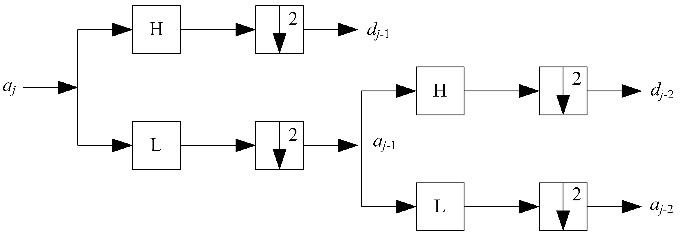
Using the Mallat algorithm, the original signal aj passes the impact response of h(n), and even samples are taken to get ; similarly, aj passes the impact response of g(n), then even samples are extracted to obtain . aj can be decomposed into a layer of low frequency components and multiple layers of high frequency components, as shown in Figure 1. The process can be expressed as:
Wavelet reconstruction is the inverse process of wavelet decomposition. The low-frequency component and the corresponding high-frequency component can be used to recover the upper low-frequency signal . Through progressive progress layer by layer, the original signal can finally be restored.
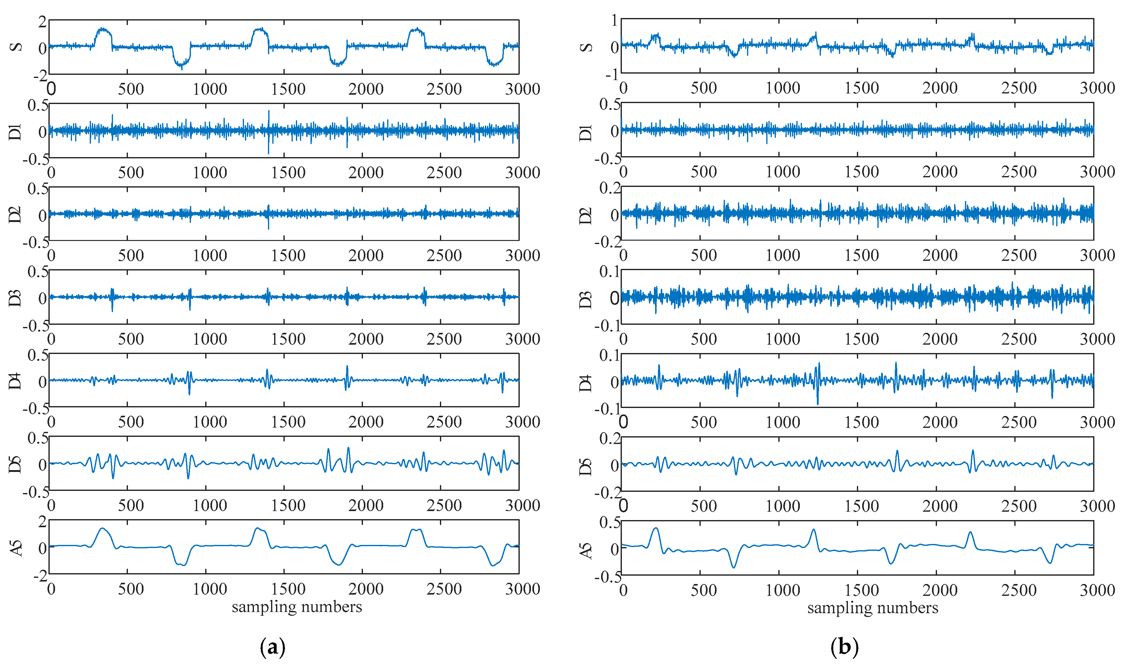
The wavelet function Symplets8 (Sym8) is used to perform 5 levels of wavelet decomposition on various current sampling signals. Taking the arcing current waveform of television as an example, the waveform of each level is shown in Figure 2. The distribution expression is:
In Figure 2, S is the original current signal, D1, D2, D3, D4, D5, and A5 represent the wavelet decomposition reconstruction coefficients of five detail signals and one approximating signal, respectively. The detail signal can highlight the characteristic of current distortion. The position where the original signal is abrupt, corresponds to the apparent singularity of the D4 and D5. The approximate signal can largely represent the overall horizontal level of original current. The waveform of A5 is approximately same as S. A 6 × 10,000 feature matrix form by A5, D5, D4, D3, D2, and D1 from low frequency to high frequency is the input sample of deep neural network.
2.2. Arc Faults Detection Based on DNN
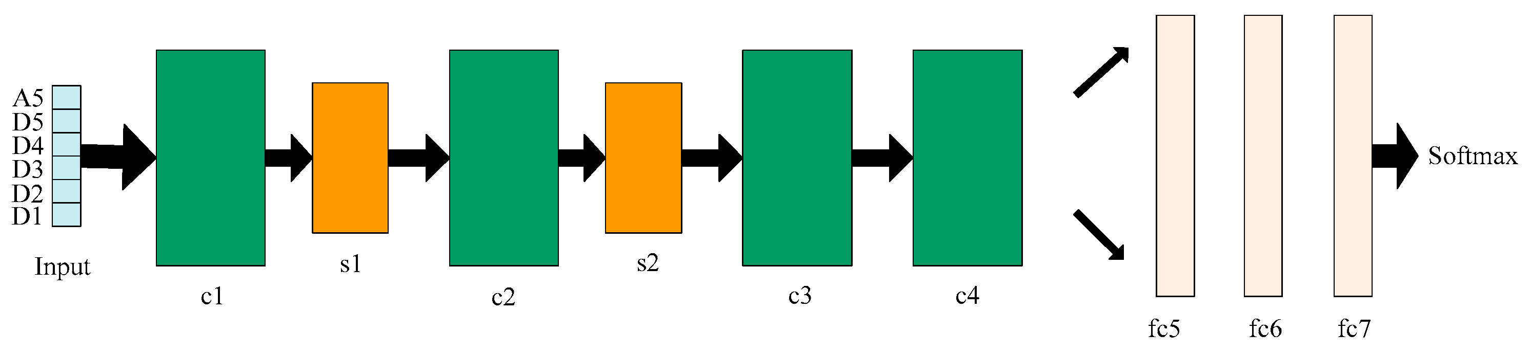
The deep neural network can simulate complex nonlinear relationships and has particular advantages in classification tasks. Combined with data type and size of input samples, the deep neural network is constructed. The structure of this model is shown in Figure 3. It consists of three different types of layers, i.e., convolutional layer (c layer), sub-sampling layer (s layer), and fully connected layer (fc layer). The first two c layers are all followed by an s layer; the third and fourth c layers are directly connected; the output of s4 is fed into three fc layers; the result of the fc7 is sent to the softmax function for two-state classification. As a whole, network structure has higher fault tolerance and more accurate data classification.
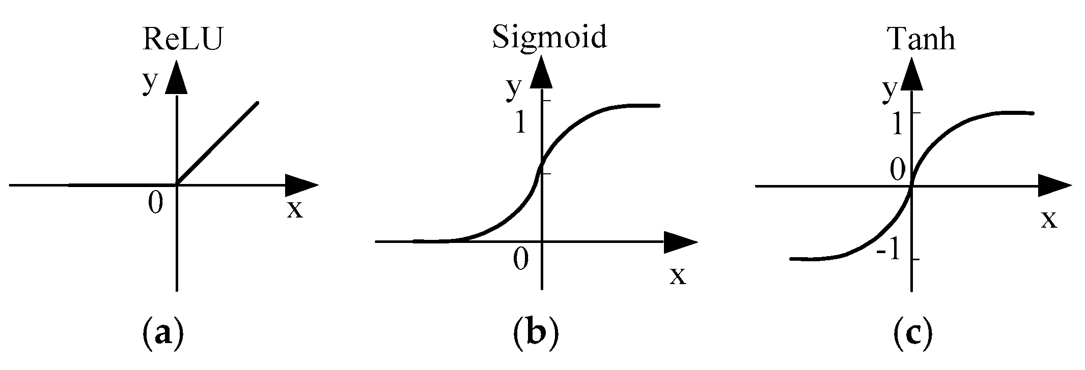
Generally, a convolutional layer is used to extract features as each convolutional unit is connected to a local patch in the feature map of the previous layer by a set of weights called filter banks [22]. Then, the result of this local weighted sum will be passed through an activation function. Compared with other non-linear function, such as Tanh and Sigmoid, the rectified linear unit (ReLU), which is a simply half-wave rectifier f(x) = max(x,0), is preferred. It can improve the training speed of neural networks without significantly affecting the generalization accuracy of model.
As shown in Figure 4a, the mapping interval of Sigmoid function is (0,1). When calculating error by backpropagation, the calculation amount of function derivative is large, and the gradient is easy to disappear. In Figure 4b, the mapping interval of Tanh function is (−1,1), and the mean value is 0. It is better than Sigmoid function in practical applications, but it is also easy for gradient to disappear. However, the ReLU function shown in Figure 4c does not have a gradient disappearance problem. It learns much faster in network than other function.
If the l layer is a convolutional layer, the output of this layer (j = 1,…, Nl) can be defined as follows:
where wc is the weight, bc is the bias, represents the output of l layer, Nl denotes the number of feature matrices of l layer, and f(·) is the activation function.
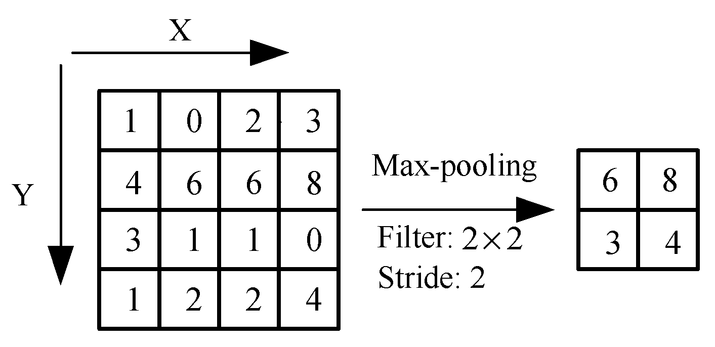
Moreover, a sub-sampling layer used between convolutional layers can reduce the feature dimensions, while ensuring that the representation is invariant to translations. Common pooling procedure have mean-pooling and max-pooling. Due to the error caused by eigenvalue extraction, the max-pooling is selected to get the maximum output in a rectangular neighborhood. The schematic is shown in Figure 5. Convolutional layer output is divided into small units by filter matrix along the X-axis and Y-axis direction, then maximum value of small units is extracted to form a new matrix. The max-pooling process is shown in:
where k is the pooling kernel, denotes the output of l layer, denotes the input of l layer, and represents the input set of feature matrices.
In DNN model, four convolutional layers all contain Local Response Normalization (LRN). It makes the adjacent features in the feature map compete locally. At the same time, features of different feature maps at the same position are compared. The response value becomes larger, the neurons with smaller feedback are suppressed more obviously, and the generalization of the model is enhanced. Its expression is as follows:
where represents the value in position of (x,y) when the number of layer is i. It is the output of upper layer, k is an offset, a is a scale factor, β is an exponent. They are respectively set to 1, 0.001/9.0 and 0.75 according to the training situation. n denotes the number of adjacent convolutional kernels at the same location. N denotes the total number of convolutional kernels.
The output feature matrices of s4 are expanded into column vectors one by one, and stacked to form a single-column eigenvector. Afterwards, this eigenvector is fed to fc5 as input. In fc5 and fc6, dropout [23] is introduced to zero the output of each neuron with probability 0.5. If the fully connection layer is layer l, the eigenvectors of the connection layer can be calculated according to:
where wd and bd represent weights and bias of the fully connection layer, and f(·) is the nonlinear activation function ReLU.
Table 1 shows details of the DNN model adjusted on the forward propagation and back propagation. Firstly, information is propagated in the feed-forward direction through different layers. The values of loss and accuracy rate are calculated. Next, back propagation algorithm is brought to minimize the error between expected value and actual value. The weight matrix is adjusted. Finally, above process are repeated until the number of epochs reaches the maximum. In order to extract local feature accurately on the local patches, the stride of the convolution unit is set to 5, the zero-padding size is set to 1, and the stride of s layer is selected to 2.
3. Mental Platform Construction and Samples Analysis
This section presents the experiment setup for collecting samples in normal and arcing state. Electrical current under different types of loads are analyzed.
3.1. Experimental Platform Construction
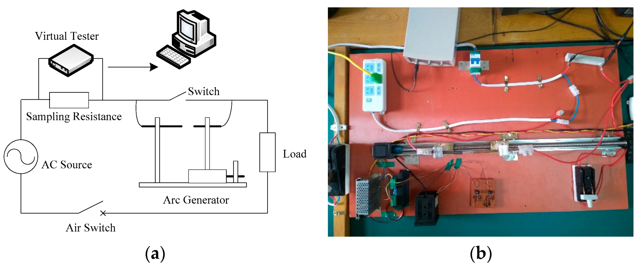
According to the description of GB14287.4-2014, electrical circuit which consists of arc generator, sampling resistor, virtual tester, and so on, supplies various domestic charges in an alternating voltage of 220 V 50 Hz. The schematic is shown in Figure 6a. The complete experimental setup is given in Figure 6b. The arc generator composed of a stepper motor that intermittently separates two electrodes, mainly simulate the arc discharge caused by line aging, poor electrical contact, and short circuit [24]. Measurements are sampled at fs = 50 kHz and stored on 8 bits through a virtual tester TiePieSCOPE HS801. Meanwhile, taking the presence of normal arc into consideration, a switch is connected in parallel with the arc generator. The switch is in the off state when collecting arc faults signals. During collecting normal current signals, the switch is operated to simulate normal arc situation.
3.2. Four Typical Load Waveform Analysis
Recently, the rapid development of electrical technology has led to a continual increase in the number of electrical products and frequent changes in the form of load connection. Loads and load change conditions of grid terminal have a great influence on arc faults occurring. As such, it is necessary to classify the characteristics of common loads.
Generally speaking, most domestic appliances are resistive loads with small inductance value; industrial equipment are mostly resistive loads, and the inductance value may be slightly larger than domestic appliances; thus, those loads can be equivalently replaced by resistive and inductive loads in the circuit.
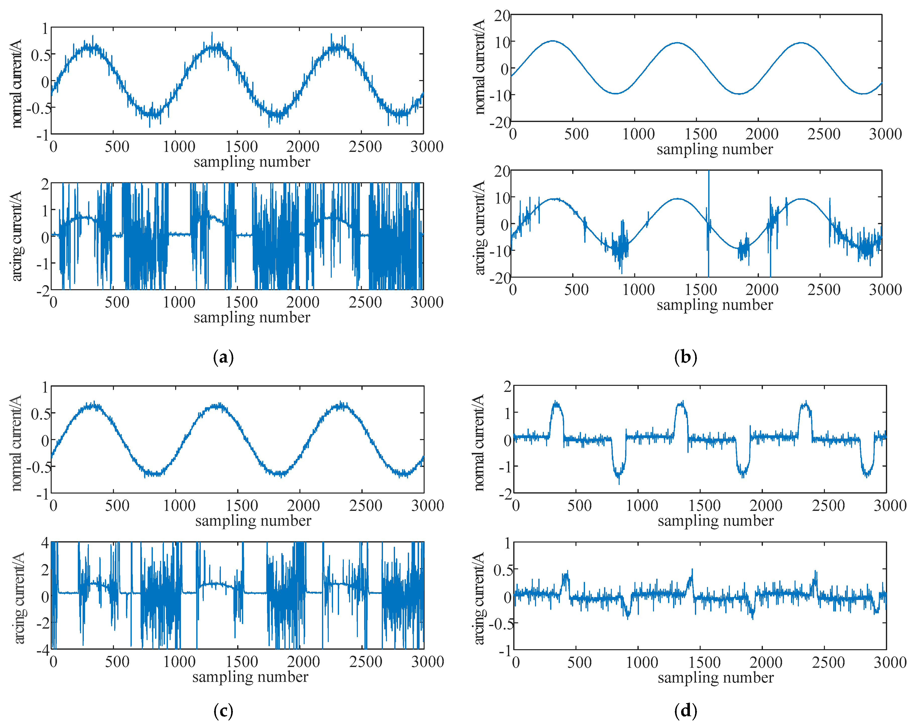
In the arc faults experiments, four typical loads including pure resistive load, pure inductive load, resistive and inductive load, and nonlinear load, are used to various loads in reality. The nature and characteristics of domestic loads are summarized in Table 2. A 200 W incandescent lamp is selected as resistive load. A 0.1 H inductance coil is selected as inductive load. The resistive and inductive load is formed by a 0.1 H inductance coil with a 200 W incandescent lamp in series. The nonlinear load is a television. And current waveforms of resistive load, inductive load, resistive and inductive load, and nonlinear load in normal and arcing conditions are shown in Figure 7, respectively, for comparison.
As is shown in Figure 7a, the phenomenon that fault current across the zero point twice every cycle is known as “flat shoulder”. There are some high-frequency interference signals on the flat shoulder, and the current rise gradient after the zero-crossing point is very high. However, in Figure 7b, the current waveform under the inductive load remains substantially sinusoidal. It is almost no flat shoulder owing to the effect of inductive energy storage. The flat shoulder phenomenon in Figure 7c is also obvious. Resistive and inductive load waveform is similar to resistive load waveform because resistive load consumes most of the energy released by the inductive load. In Figure 7d, for television, the waveform characteristics of normal current and arcing current are very similar. Compared with normal current, the amplitude of fault current is reduced, and the high-frequency noise distribution is wider.
4. Experimental Results and Analysis
The personal computer in this study adopts an Intel(R) Core(TM) I7-7700HQ as the processor and running memory of 16 GB. Under the Ubuntu 16.04 operating system, the DNN model was built using the tensorflow-gpu configuration of Pycharm Communtiy 2018.2 software. The Adam optimizer, which uses momentum to improve traditional gradient descent and promote hyperparametric dynamic adjustment, is selected in this model [25]. We found that the training and test results are better when the learning rate is 0.001 and the size of training batch is 100.
4.1. Training Results
The loss function used to measure model prediction quality is an important parameter for model learning. The loss function can be written as:
where represents the ith value of output vector , is the ith value of actual label, and N is the number of training samples.
The performance of this model is measured in each iteration progress by calculating the cross entropy between predicted label and actual label. The optimization procedure is guided by minimizing the cross entropy as quickly as possible through gradually adjusting parameters (weights and bias) of network.
Data sets of normal state and arcing state are labeled using the one-hot encoding for easy class comparison and performance measure. The label vector is composed of 0 and 1. Index position where the maximum value 1 is located is the category label. The index position of predicted label and actual label are compared to obtain a true or false matrix. The ratio of the true value can be calculated to get accuracy. The accuracy can be defined as follows:
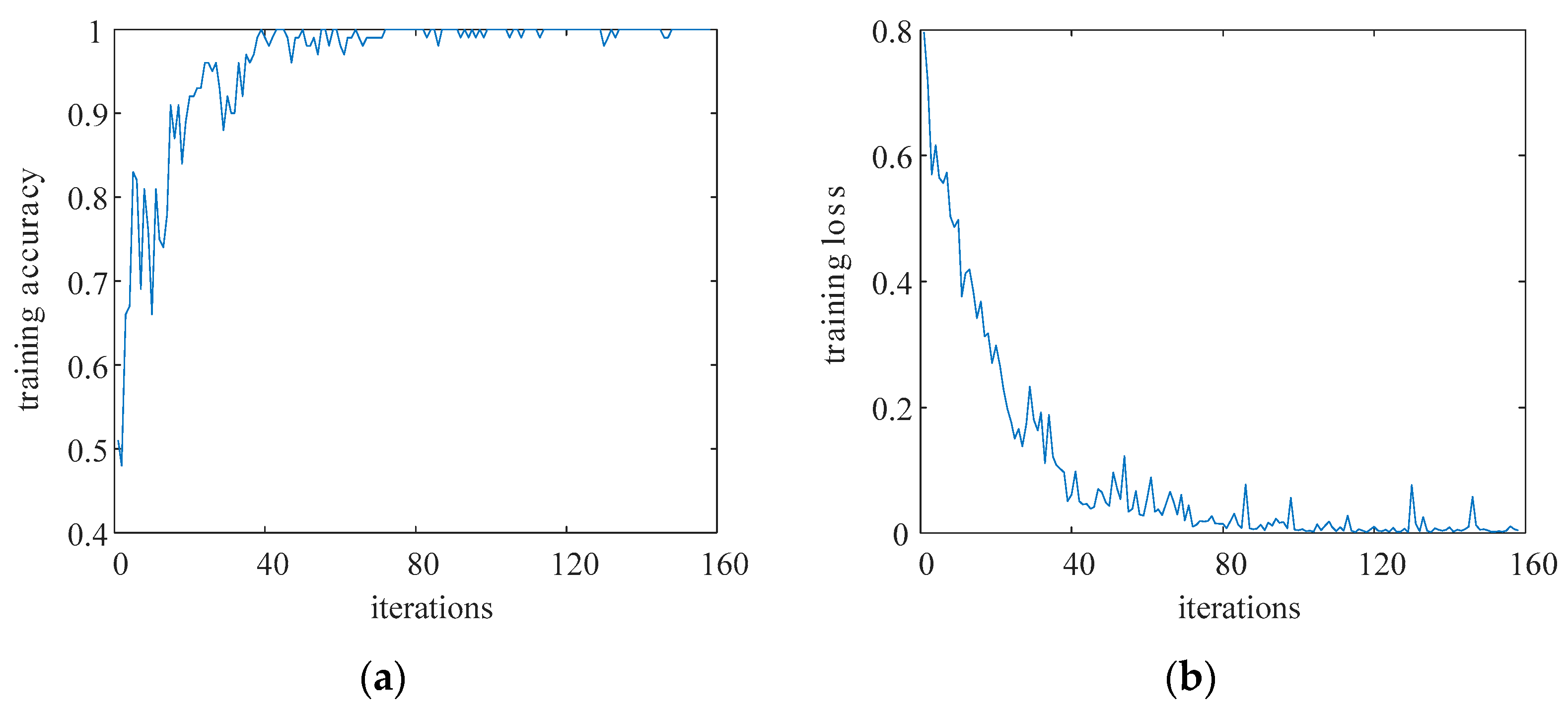
From 9600 samples, 8000 samples are randomly selected as training samples for feeding into deep neural network. After 2 epochs (total 160 iterations), the training process is over, and the changes of training accuracy and loss are shown in Figure 8. Obviously, with the increase of training iterations, the training accuracy rate has an overall upward trend, while the training loss value shows a general downward trend. After iterating 70 times, the accuracy basically converges, and the loss value is basically stabilized at about 0.012.
4.2. Test Results
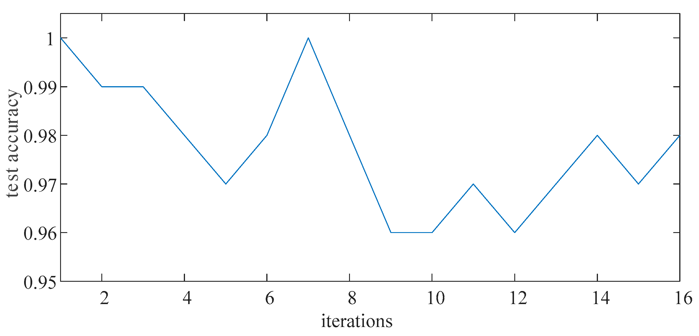
1600 test samples are randomly shuffled and feed into the trained DNN model for evaluating and validating diagnostic accuracy. As can be seen from Figure 9, the test results are generally maintained at around 97.75%.
However, in Table 3, it can be clearly seen that the test results of different loads are different. The average accuracy of inductive load test sample is 0.9225, the average accuracy of resistive and inductive load test sample is 0.995, the average accuracy of resistive load test sample is 0.9925, and the average accuracy of nonlinear load test sample is 1. In comparison to resistive load and restive and inductive load, current waveform of inductive load is short of natural zero crossing. It means that detecting arc faults in this condition is inherently more difficult. In addition, the test result of nonlinear load is good enough. The arc faults detection under the condition of nonlinear load is not a problem. Collectively, these comparisons validate the accuracy of the DNN model in series arc faults detection.
4.3. Comparison with Prior Methods
In the aspects of framework, model structure, application range and detection accuracy, the comparison of our method with some prior methods are summarized in Table 4.
Liu et al. [26] use discrete wavelet transform to obtain the time-frequency domain characteristics, and some measured data are feed into a radial basis function neural network (RBFNN) for training. Method proposed in this paper could be applied to resistive loads, inductive loads, resistive and inductive loads, and nonlinear loads. It is more general than methods presented in [20,26]. Wang et al. [27] proposed a sparse representation and fully connected neural network (SRFCNN) method. They utilize six fully connection layers to classify and train a large data set which contains more than 15,000 samples. In resistive load condition, they determined that the classification accuracy can reach above 95% with 160 epochs or less. The training procedure in our method consumes less epochs to achieve good diagnostic accuracy than [26]. The detection of series ac arc faults is requested to have high accuracy. Test results indicates that our method has higher precision than methods [20,27].
5. Conclusions
On the basis of the ability of deep neural networks to automatically learn essential features from a large number of samples data, a series arc fault detection method based on wavelet transform and deep convolutional neural network is proposed. According to the GB14287.4-2014 standard, current signals are sampled by four typical loads under 220V distribution system. After analyzing the arc faults current characteristics, wavelet coefficient sequences are used to form the input matrix of deep neural network. Testing results of the DNN model show that this model can operate effectively and can be applied to multiple load type applications. Future work will continue to improve accuracy. Special loads, combined loads and typical interference loads will be tested according to GB14287.4-2014 standard to fully assess the possible performance in this method.
Author Contributions
Conceptualization, Q.Y. and Y.Y.; Methodology, Y.Y.; Software, Y.H.; Validation, Q.Y., Y.Y. and Y.H.; Formal analysis, Q.Y.; Investigation, Y.H.; Resources, Q.Y. and Y.Y.; Data curation, Y.H.; Writing—original draft preparation, Y.H.; Writing—review and editing, Q.Y.; Visualization, Y.Y.; Project Administration: Q.Y.; Funding Acquisition: Q.Y. All authors have read and agreed to the published version of the manuscript.
Funding
This research was funded by the National Natural Science Foundation of China (61601172) and the Postdoctoral Science Foundation of China (2018M641287).
Acknowledgments
Thanks to all the authors for their joint efforts, thanks to the reviewers for their valuable comments, and thanks for the care and help of editors all the time.
Conflicts of Interest
The authors declare no conflict of interest.
References
- Gregory, G.D.; Scott, G.W. The arc-fault circuit interrupter, an emerging product. In Proceedings of the 1998 IEEE Industrial and Commercial Power Systems Technical Conference, Edmonton, AB, Canada, 3–8 May 1998; Volume 34, pp. 928–933. [Google Scholar]
- Giovanni, A.; Antonio, C.; Valentina, C.; Giuseppe, P. Experimental characterization of series arc faults in AC and DC electrical circuits. In Proceedings of the 2014 IEEE International Instrumentation and Measurement Technology Conference (I2MTC), Montevideo, Uruguay, 12–15 May 2014; pp. 1015–1020. [Google Scholar]
- Giovanni, A.; Antonio, C.; Valentina, C.; Dario, D.C.; Salvatore, N.; Giovanni, T. Arc Fault Detection Method Based on CZT Low-Frequency Harmonic Current Analysis. IEEE Trans. Instrum. Meas. 2017, 66, 888–896. [Google Scholar] [CrossRef]
- Kostyantyn, K.; Bei, G.; Aslakson, J. A Low-Cost Power-Quality Meter with Series Arc-Fault Detection Capability for Smart Grid. IEEE Trans. Power. Deliver. 2013, 28, 1584–1591. [Google Scholar] [CrossRef]
- Guan, H.L.; Wang, B.; Zhao, Z.Z.; Bimenyimana, S.; Wang, Q.L. Arc Fault Current Signal’s Power Spectrum Characteristics and Diagnosis Based on Welch Algorithm. Int. J. Eng. Sci. Comp. 2016, 5, 2852–2857. [Google Scholar]
- Lezama, J.; Schweitzer, P.; Tisserand, E.; Humbert, J.; Weber, S.; Joyeux, P. An embedded system for AC series arc detection by inter-period correlations of current. Electric Power Syst. Res. 2015, 129, 227–234. [Google Scholar] [CrossRef]
- Lu, Q.W.; Ye, Z.Y.; Zhang, Y.L.; Wang, T.; Gao, Z.X. Analysis of the Effects of Arc Volt–Ampere Characteristics on Different Loads and Detection Methods of Series Arc Faults. Energies 2019, 12, 323. [Google Scholar] [CrossRef] [Green Version]
- Ji, H.K.; Wang, G.; Kim, W.H.; Kil, G.S. Optimal Design of a Band Pass Filter and an Algorithm for Series Arc Detection. Energies 2018, 11, 992. [Google Scholar] [CrossRef] [Green Version]
- Ilman, A.F. Low Voltage Series Arc Fault Detection with Discrete Wavelet Transform. In Proceedings of the 2018 International Conference on Applied Engineering (ICAE), Batam, Indonesia, 3–4 October 2018. [Google Scholar]
- Jovannovic, S.; Chahid, A.; Lezama, J.; Schweitzer, P. Shunt active power filter-based approach for arc fault detection. Electric Power Syst. Res. 2016, 141, 11–21. [Google Scholar] [CrossRef]
- Chen, C.K.; Guo, F.Y.; Liu, Y.L.; Wang, Z.Y.; Chen, Y.J.; Liang, H.H. Recognition of series arc fault based on the Hilbert Huang Transform. In Proceedings of the 2015 IEEE 61st Holm Conference on Electrical Contacts (Holm), San Diego, CA, USA, 11–14 October 2015; pp. 324–330. [Google Scholar]
- Liu, J.T.; Zhou, K.F.; Hu, Y. EMD-WVD Method Based High-Frequency Current Analysis of Low Voltage Arc. In Proceedings of the 2018 Condition Monitoring and Diagnosis (CMD), Perth, Australia, 23–26 September 2018. [Google Scholar]
- Zhang, S.W.; Zhang, F.; Wang, Z.J.; Gu, H.Y.; Ning, Q. Series Arc Fault Identification Method Based on Energy Produced by Wavelet Transformation and Neural Network. Trans. China Electrotech. Soc. 2014, 29, 290–295. [Google Scholar]
- Yin, Z.D.; Wang, L.; Gao, W.; Zhang, Y.J.; Gao, Y. A Novel Arc Fault Detection Method Integrated Random Forest, Improved Multi-scale Permutation Entropy and Wavelet Packet Transform. Electronics 2019, 8, 396. [Google Scholar] [CrossRef] [Green Version]
- Krizhevsky, A.; Sutskever, I.; Hinton, G. ImageNet classification with deep convolutional neural networks. Commun. ACM 2012, 60, 84–90. [Google Scholar] [CrossRef]
- Liu, W.B.; Wang, Z.D.; Liu, X.H.; Zeng, N.Y.; Liu, Y.R.; Alsaadi, F.E. A survey of deep neural network architectures and their applications. Neurocomputing 2017, 234, 11–26. [Google Scholar] [CrossRef]
- Guo, M.F.; Zeng, X.D.; Chen, D.Y.; Yang, L.C. Deep-Learning-Based Earth Fault Detection Using Continuous Wavelet Transform and Convolutional Neural Network in Resonant Grounding Distribution Systems. IEEE Sens. J. 2018, 18, 1291–1300. [Google Scholar] [CrossRef]
- Karaduman, G.; Karakose, M.; Akin, E. Deep Learning Based Arc Detection in Pantograph-catenary Systems. In Proceedings of the 10th International Conference on Electrical and Electronics Engineering (ELECO), Bursa, Turkey, 30 November–2 December 2017; pp. 904–908. [Google Scholar]
- Siegel, J.E.; Pratt, S.; Sun, Y.; Sarma, S.E. Real-time Deep Neural Networks for internet-enabled arc-fault detection. Eng. Appl. Artif. Intell. 2018, 74, 35–42. [Google Scholar] [CrossRef] [Green Version]
- Yu, Q.F.; Huang, G.L.; Yang, Y.; Sun, Y.Z. Series fault arc detection method based on AlexNet deep learning network. J. Electric Meas. Instrust. 2019, 33, 145–152. [Google Scholar] [CrossRef]
- Daubechies, I. Ten Lectures on Wavelets; Posts & Telecom Press: Beijing, China, 2017; pp. 16–95. ISBN 978-7-115-43898-0. [Google Scholar]
- LeCun, Y.; Bengio, Y.; Hinton, G. Deep learning. Nature 2015, 521, 436–444. [Google Scholar] [CrossRef] [PubMed]
- Srivastava, N.; Hinton, G.; Krizhevsky, A.; Sutskever, I.; Salakhutdinov, R. Dropout: A Simple Way to Prevent Neural Networks from Overfitting. J. Mach. Learn. Res. 2014, 15, 1929–1958. [Google Scholar]
- Mehrdad, D.; Abdelhamid, R.; Ahmed, E.H. Comprehensive Modulation and Classification of Faults and Analysis Their Effect in DC Side of Photovoltaic System. Energy Power Eng. 2013, 5, 230–236. [Google Scholar] [CrossRef]
- Diederik, P.K.; Jimmy, L.B. Adam: A Method for Stochastic Optimizer. In Proceedings of the 3rd International Conference on Learning Representations, San Diego, CA, USA, 7–9 May 2015. [Google Scholar]
- Liu, Y.; Wu, C.; Wang, Y. Detection of serial arc fault on low-voltage indoor power lines by using radial basis function neural network. Int. J. Electric Power Energy Syst. 2016, 83, 149–157. [Google Scholar] [CrossRef]
- Wang, Y.; Zhang, F.; Zhang, S. A New Methodology for Identifying Arc Fault by Sparse Representation and Neural Network. IEEE Trans. Instrum. Meas. 2018, 67, 2526–2537. [Google Scholar] [CrossRef]
Figure 1.
Multiscale wavelet decomposition.

Figure 2.
Wavelet decomposition reconstruction signal diagram: (a) normal current; (b) arcing current.
Figure 2.
Wavelet decomposition reconstruction signal diagram: (a) normal current; (b) arcing current.

Figure 3.
Structure of the deep neural network.

Figure 4.
Activation function curve: (a) ReLU; (b) Sigmoid; (c) Tanh.

Figure 5.
Principle of max-pooling.

Figure 6.
Series arc faults experiment platform: (a) schematic; (b) actual platform.

Figure 7.
Normal current and arcing current waveforms of four kinds of loads: (a) resistive load; (b) inductive load; (c) resistive and inductive load; (d) nonlinear load.
Figure 7.
Normal current and arcing current waveforms of four kinds of loads: (a) resistive load; (b) inductive load; (c) resistive and inductive load; (d) nonlinear load.

Figure 8.
Training results of model. (a) Training accuracy; (b) Training loss.

Figure 9.
Test results of model.


Table 1.
Deep neural network (DNN) configuration of each layer.
| Layer Types | Size of Convolution Kernel | Sub-Sampling Layer | Pad | Stride | Size of Output Feature Matrix |
|---|---|---|---|---|---|
| input | - | - | - | - | 6 × 10,000-1 |
| c1 | 6 × 6 | - | 1 | 5 | 2 × 2000-32 |
| s1 | 2 × 2 | Max-pooling | 0 | 2 | 1 × 1000-32 |
| c2 | 1 × 6 | - | 1 | 5 | 1 × 200-64 |
| s2 | 1 × 2 | Max-pooling | 0 | 2 | 1 × 100-64 |
| c3 | 1 × 6 | - | 1 | 5 | 1 × 20-128 |
| c4 | 1 × 6 | - | 1 | 5 | 1 × 4-64 |
| fc5 | - | - | - | - | 256 × 1-1 |
| fc6 | - | - | - | - | 256 × 1-1 |
| fc7 | - | - | - | - | 2 × 1-1 |
Table 2.
Experimental load and parameters.
| Load Properties | Experimental Loads | Load Parameters | Normal (Sample Number) | Fault (Sample Number) |
|---|---|---|---|---|
| Resistive load | filament lamp | 200 W | 1200 | 1200 |
| Inductive load | inductance coil | 0.1 H | 1200 | 1200 |
| Resistive and inductive load | filament lamp+ inductance coil | 200 W + 0.1 H | 1200 | 1200 |
| Nonlinear load | television | 120 W | 1200 | 1200 |
Table 3.
Test results of different loads.
| Test Iteration | Resistive Load | Inductive Load | Resistive and Inductive Load | Nonlinear Load |
|---|---|---|---|---|
| 1 | 1 | 0.94 | 1 | 1 |
| 2 | 0.95 | 0.91 | 0.99 | 1 |
| 3 | 1 | 0.92 | 0.99 | 1 |
| 4 | 1 | 0.92 | 0.99 | 1 |
| Average | 0.995 | 0.9225 | 0.9925 | 1 |
Table 4.
Comparison with period methods.
| Methods | Framework | Model Structure | Application Range | Detection Accuracy |
|---|---|---|---|---|
| Liu et al. [26] | combine the DWT with the three-layer resolution and signal energy to RBFNN. | not introduced in the paper. | resistive, inductive, resistive and inductive loads. | not introduced |
| Wang et al. [27] | apply the sparse coefficients to six fully connection layers. | [250, a, b, c, d, 10] a, b, c, d are the neuron numbers. | resistive, inductive, capacitive, nonlinear loads. | 97.6% |
| Yu et al. [20] | utilize current data measured by experiments to the improved AlexNet. | five convolution layers, three pooling layers, three full connection layers. | resistive, inductive, resistive and inductive loads. | 85.25% |
| Our method | employ data decomposed by DWT to the DNN model. | four convolution layers, two pooling layers, three full connection layers. | resistive, inductive, resistive and inductive, nonlinear loads. | 97.75% |
© 2019 by the authors. Licensee MDPI, Basel, Switzerland. This article is an open access article distributed under the terms and conditions of the Creative Commons Attribution (CC BY) license (http://creativecommons.org/licenses/by/4.0/).
Share and Cite
MDPI and ACS Style
Yu, Q.; Hu, Y.; Yang, Y. Identification Method for Series Arc Faults Based on Wavelet Transform and Deep Neural Network. Energies 2020, 13, 142. https://0-doi-org.brum.beds.ac.uk/10.3390/en13010142
AMA Style
Yu Q, Hu Y, Yang Y. Identification Method for Series Arc Faults Based on Wavelet Transform and Deep Neural Network. Energies. 2020; 13(1):142. https://0-doi-org.brum.beds.ac.uk/10.3390/en13010142
Chicago/Turabian StyleYu, Qiongfang, Yaqian Hu, and Yi Yang. 2020. "Identification Method for Series Arc Faults Based on Wavelet Transform and Deep Neural Network" Energies 13, no. 1: 142. https://0-doi-org.brum.beds.ac.uk/10.3390/en13010142
Note that from the first issue of 2016, this journal uses article numbers instead of page numbers. See further details here.